A comprehensive scenario of the thermodynamic anomalies of water using the TIP4P/2005 model

Abstract

The striking behavior of water has deserved it to be referred to as an “anomalous” liquid. The water anomalies are greatly amplified in metastable (supercooled and/or stretched) regions. This makes difficult a complete experimental description since, beyond certain limits, the metastable phase necessarily transforms into the stable one. Theoretical interpretation of the water anomalies could then be based on simulation results of well validated water models. But the analysis of the simulations has not yet reached a consensus. In particular, one of the most popular theoretical scenarios —involving the existence of a liquid-liquid critical point (LLCP)— is disputed by several authors. In this work we propose to use a number of exact thermodynamic relations which may shed light on this issue. Interestingly, these relations may be tested in a region of the phase diagram which is outside the LLCP thus avoiding the problems associated to the coexistence region. The central property connected to other water anomalies is the locus of temperatures at which the density along isobars attain a maximum (TMD line) or a minimum (TmD). We have performed computer simulations to evaluate the TMD and TmD for a successful water model, namely TIP4P/2005. We have also evaluated the vapor-liquid spinodal in the region of large negative pressures. The shape of these curves and their connection to the extrema of some response functions, in particular the isothermal compressibility and heat capacity at constant pressure, provide a very useful information which may help to elucidate the validity of the theoretical proposals. In this way we are able to present for the first time a comprehensive scenario of the thermodynamic water anomalies for TIP4P/2005 and their relation to the vapor-liquid spinodal. The overall picture shows a remarkable similarity with the corresponding one for the ST2 water model, for which the existence of a LLCP has been demonstrated in recent years. It also provides a hint as to where the long-sought for extrema in response functions might become accessible to experiments.

I Introduction

The physical properties of water at ambient conditions are markedly different from those of other liquids. It is widely known that the density of liquid water at a fixed pressure exhibits a maximum at the so-called temperature of maximum density (TMD). In particular, at atmospheric pressure, the TMD is approximately 4 ^∘C. Below this temperature the water’s expansivity, $\alpha$, is negative in striking contrast with “normal” liquids where $\alpha$ is always positive. Other thermodynamic response functions, such as the isothermal compressibility, $\kappa_{T}$, or the isobaric heat capacity $C_{p}$ also show an unusual behavior.Debenedetti (2003) On supercooling, these anomalies are enhanced. In particular, the isothermal compressibility seems to diverge at 228 K.Speedy and Angell (1976)

Several scenarios have been proposed to account for the water anomalies and their magnification at temperatures below the melting point.Speedy (1982); Poole et al. (1992); Sastry et al. (1996); Angell (2008) In the stability limit conjecture (SLC),Speedy (1982) the increase of the response functions in the supercooled region is ascribed to a continuous retracing line of instability that delimits the supercooled and stretched metastable states. The second critical point scenario assumes that there is a liquid-liquid coexistence terminating at a critical point (LLCP).Poole et al. (1992) The response functions would reach a peak and converge towards the Widom line (the line of the maxima of the correlation length) emanating from the LLCP.Sciortino et al. (1997); Xu et al. (2005) Finally, it has been shown that thermodynamic consistency explains the existence of peaks in the response functions as a mere consequence of the presence of density anomalies. In this case there is no singular behavior, hence the name of singularity-free (SF) scenario.Sastry et al. (1996) Notice that the SF interpretation can also be seen as the second critical-point hypothesis with the LLCP occurring at zero temperature.

The experimental testing of these scenarios is extremely difficult, if not impossible, because of the difficulties to access the “no man’s land” region that lies below the temperature at which water spontaneously freezes. Crystallization may be inhibited by confining water in nanosized samples, but it is unclear whether surface effects could influence the outcome of the experiments.Zanotti et al. (2005); Mallamace et al. (2007, 2008) Different experimental approaches have been proposed to circumvent the problems associated with the bulk water no man’s landMishima and Stanley (1998a, b); Bellissent-Funel (1998); Soper (2000); Mishima and Suzuki (2002); Souda (2006); Banerjee et al. (2009); Taschin et al. (2013); Pallares et al. (2014); Sellberg et al. (2014); Seidl et al. (2015) (see also a recent reviewCaupin (2015) on this topic). They have provided very important information on the behavior of water at extreme conditions (deep supercooling and/or high negative pressures). Although the experiments seem to be consistent and support the appearance of a liquid-liquid transition, their interpretation is not conclusive.

Theoretical work has shown that the slope of the TMD loci determines the behavior of the thermodynamic response functions. Exact thermodynamic relations relate the shape of the TMD to that of other water anomalies. It is well known that the TMD of liquid water is a negatively sloped function in a p-T diagram. If the negative slope would extend to large negative pressures (SLC scenario), it would meet the vapor-liquid spinodal. In such a case, thermodynamic consistency requiresDebenedetti and D’Antonio (1986) that the spinodal would retrace at the intersection point. On the other hand, the TMD could change its slope leading to a nose-shaped function (LLCP and SF scenarios). It has been demonstrated that a positively sloped TMD line cannot cross a positively sloped spinodal in a thermodynamically consistent phase diagram and that the turning point of the TMD must intersect the locus of isothermal compressibility extrema.Sastry et al. (1996) In summary, the study of the TMD of stretched water may give insight to the validity of the hypothesis proposed to explain the water anomalies. Recent measurements of the speed of soundPallares et al. (2014) have enabled to extend considerably our knowledge of the TMD in the region of large negative pressures.Pallares et al. (2016) These results indicate that the slope of the TMD becomes increasingly more negative as the pressure decreases and strongly suggest that the experimental TMD is about to reach a retracing point. Unfortunately, bubble nucleation prevents carrying this study further.

Given the experimental difficulties, it is clear that molecular simulation may be an alternative for our purpose. Most of the computer simulation studies using realistic water models seem to support the existence of the liquid–liquid separation. The seminal work of Poole et al.Poole et al. (1992) focused on the ST2 water model.Stillinger and Rahman (1974) Some of the features of the ST2 model allow a thorough investigation of the supercooled region. Because of this, the model has been widely used in the study of the liquid-liquid phase transition. Most simulations using ST2Poole et al. (1993); Sciortino et al. (1997); Xu et al. (2005); Brovchenko et al. (2005); Liu et al. (2009); Sciortino et al. (2011); Liu et al. (2012); Kesselring et al. (2012); Poole et al. (2013); Palmer et al. (2013, 2014); Yagasaki et al. (2014); Palmer et al. (2016) seem to have unambiguously demonstrated the existence of a LLCP although this interpretation has been challenged by Limmer and Chandler.Limmer and Chandler (2011); Chandler (2016) But the advantages of the model for the study of the supercooled region (among them, a high value for the TMD) are closely related to its major drawback: ST2 is known to produce an over-structured liquid compared to real water. Thus, there is no compelling evidence that the behavior of metastable water can be described by ST2.Liu et al. (2009)

Alternative successful water models can indeed be found in the literature though they are not free of objections. SPC/EBerendsen et al. (1987) is a widely used model showing excellent predictions for a number of water properties in the liquid region.Vega and Abascal (2011) However, its bad performance in locating the temperature of maximum density (TMD), the melting temperature, T_m, and the isothermal compressibility minimumPi et al. (2009), seem to discourage its use to investigate the supercooled region. Since TIP5PMahoney and Jorgensen (2000); Rick (2004) provides very good estimates of both the TMD and T_m, it has been used in simulation studies attempting to disclose the behavior of metastable liquid water.Yamada et al. (2002); Paschek (2005); Brovchenko et al. (2005); Xu et al. (2005); Brovchenko et al. (2005); Yagasaki et al. (2014) However, the excellent performance of the model at ambient conditions is not preserved when one moves away of this region. This failure is particularly serious because it is a signal that the results for the response functions cannot be satisfactory.Vega and Abascal (2011) Moreover, TIP5P gives a very poor estimate of the density of hexagonal ice and, hence, of the density and other properties of a possible low density phase in a liquid-liquid coexistence.

It has been demonstrated Vega et al. (2005); Abascal and Vega (2007a, b) that the TIP4P geometry is more appropriate than that of three-site models —such as SPC— or five-site models —like TIP5P— to account for the TMD and the liquid-solid equilibrium of water. These studies followed an increasing interest in re-parametrized TIP4P models.Horn et al. (2004); Abascal et al. (2005); Abascal and Vega (2005) Among these, TIP4P/2005Abascal and Vega (2005) seems to produce a better overall agreement with experiment for a large number of properties of water in condensed states.Vega et al. (2009); Vega and Abascal (2011) Moreover, TIP4P/2005 results are quite accurate for properties relevant to the study of metastable water, namely water anomaliesPi et al. (2009) and equation of state of supercooled water.Abascal and Vega (2011) Finally, the model gives a quantitative account of recent measurements of the speed of sound of doubly metastable (supercooled and stretched) water.Pallares et al. (2014)

From the above arguments it seems then that TIP4P/2005 is the ideal candidate for the study of the water anomalies in the supercooled region. It may come as a surprise that only a reduced number of works have been devoted to this issue,Abascal and Vega (2010); Sumi and Sekino (2013); Limmer and Chandler (2013); Overduin and Patey (2013); Yagasaki et al. (2014); Bresme et al. (2014); Russo and Tanaka (2014); Overduin and Patey (2015); Singh et al. (2016) probably because the model has also some limitations mainly derived from the large structural relaxation times at deeply supercooled states. Abascal and VegaAbascal and Vega (2010) proposed that the model exhibits a LLCP at 193 K and reported a case of a liquid-liquid separation (low- and high-density) below the second critical point. Even though Overduin and PateyOverduin and Patey (2013) argued that longer simulations (8 $\mu$s for 500 molecules, instead of 400 ns) were necessary to obtain well converged density distributions at those conditions, a number of authorsSumi and Sekino (2013); Yagasaki et al. (2014); Bresme et al. (2014); Russo and Tanaka (2014) confirmed the rest of the results presented in Ref. Abascal and Vega, 2010. The study of Overduin and Patey does not essentially contradict the results of Abascal and Vega if the suggested LLCP of TIP4P/2005 would be slightly shifted towards lower temperatures. This is in line with the critical temperature reported for this model by Sumi and SekinoSumi and Sekino (2013) (182 K) and Yagasaki et al.Yagasaki et al. (2014) (185 K). Interestingly, a two-structure equation of state consistent with the presence of a LLCP provides a very similar critical temperature.Bresme et al. (2014); Singh et al. (2016) Therefore, it would be of great interest to perform a simulation study using advanced sampling methods to unambiguously check the existence of a LLCP for this model (similar to that successfully accomplished for ST2Palmer et al. (2014)). However, the work of Overduin and Patey clearly indicates that such study would be extremely costly in computer time.

In this work we propose to circumvent the question of the existence of a LLCP and focus on the related issue of the shape of the TMD and its relation to other water anomalies. As shown above, the study not only involves calculations in the supercooled and/or stretched region outside the proposed critical region, but it may also provide a complete perspective of the scenario of water anomalies. Although the study is highly demanding in computer resources, it is still affordable. We also note that, regardless of the nature of the phase diagram of TIP4P/2005 liquid at low temperature (real or virtual critical point, …), the region we consider in the present paper includes the one relevant for experiments on bulk water. It can therefore serve as a guide for future measurements.

II Methods

All simulations (except those intended for the calculation of the vapor-liquid spinodal) have been performed with 4 000 TIP4P/2005 water molecules in the isothermal-isobaric $NpT$ ensemble using the Molecular Dynamics package GROMACS 4.6van der Spoel et al. (2005); Hess et al. (2008) with a 2 fs timestep. Long range electrostatic interactions have been evaluated with the smooth Particle Mesh Ewald method.Essmann et al. (1995) The geometry of the water molecules has been enforced using ad hoc constraints, in particular, the LINCS algorithm.Hess et al. (1997); Hess (2008) To keep the temperature and pressure constant, the Nosé-Hoover thermostatNosé (1984); Hoover (1985) and an isotropic Parrinello-Rahman barostat have been appliedParrinello and Rahman (1981) with 2 ps relaxation times.

Most of our calculations intended to evaluate the extrema of thermodynamic properties, and we have adapted our strategy according to this goal. First, we calculated the desired property at regular intervals along isotherms/isobars to provide a rough estimate of the position of the maximum or minimum. Then we ran additional points to precisely locate it. We monitored the uncertainties along the simulation and extended the runs until the differences between the consecutive points were larger than the statistical uncertainty. Thus, the required simulation times varied widely for the different properties and state points. Since most of the calculations correspond to regions where the relaxation of the system is quite slow, the length of the simulations is often of the order of a few hundreds of ns, reaching 1.3 $\mu$s for the longest run. Despite the careful monitoring of the runs to save computer resources, the required simulation times together with the use of a relatively large system size implies an important computational effort (equivalent to more than 300 000 hours of 2.6 GHz Xeon cores) that has been achieved by means of a GPU-based supercomputer.

The uncertainty on each measurement has been calculated using a method proposed by Hess.Hess (2002) The trajectory is divided in blocks, the average for each block is calculated and the error is estimated as the standard deviation of the block averages. Also, an analytical block average curve is obtained by fitting the autocorrelation between block averages to a sum of two exponentials. In this way, the calculated uncertainties lead to an asymptotic curve only if the trajectory is long enough so that the blocks are uncorrelated. In summary, the procedure not only provides an estimate of the error but also sheds light on the convergence of the trajectory. An example of the application of the method is given as supplementary material.epa

III Results

Although TIP4P/2005 provides quite acceptable results for the density of water at positive pressures (also including the supercooled regionAbascal and Vega (2011)), its performance at negative pressures has not been thoroughly assessed (see however Refs. Pallares et al., 2014 and Pallares et al., 2016). Very recently, an experimental equation of state for water down to -120 MPa has been reported.Pallares et al. (2016) This allows to check for the first time the predictions for the equation of state in the large negative pressures region. predictions The numerical values of the density along some isobars for the TIP4P/2005 model are given as supplementary material.epa Figure 1 shows that the agreement between simulation results and experiment is excellent although the departures increase with decreasing pressures. As a consequence, the prediction for the TMD is slightly shifted, the difference at -80 MPa being about 7 degrees.

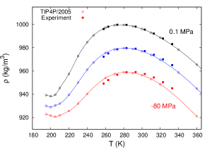
Figure 1: Densities predicted by the TIP4P/2005 model compared to recent experimental dataPallares et al. (2016) for the 0.1 MPa, -40 MPa and -80 MPa isobars.

In the positive pressures region, the simulation data show a maximum density for isobars up to a pressure of 200 MPa. In accordance with experiment,Angell and Kanno (1976) at increasing pressures the TMD shifts to lower temperatures. At negative pressures the slope of the TMD becomes increasingly negative until the curve retraces (point A in Fig 2). From the turning point to highly negative pressures the TMD has a positive slope. This result has already been reported in previous works for much smaller samples.Agarwal et al. (2011); Pallares et al. (2016) Our results for the larger system are very similar to the previous ones and indicate that finite size effects in this region (if any) are quite small (see supplemental materialepa ). The largest (negative) pressure for which we have been able to calculate the temperature of maximum density is -170 MPa. Unfortunately, at -200 MPa the system cavitated for several runs using 4 000 water molecules. However, using 500 molecules allowed us to perform short runs before the system cavitated so it is possible an approximate calculation of the densities and the approximate position of the TMD at this pressure.

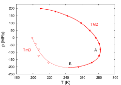
Figure 2: Locus of density maxima (TMD, thick line) and minima (TmD, thin line). Points A and B mark the turning point of the TMD curve and the point at which the TMD and TmD lines meet, respectively.

The isobars at negative pressures also exhibit a temperature of minimum density, TmD. However, in the positive pressures region, only the 0.1 MPa curve shows the density minimum. In all cases, the minimum is quite shallow and it is barely appreciable, especially in the case of the -125 MPa and -170 MPa isobars. Fig. 3 show a detail of these isobars clearly demonstrating the existence of density minima.

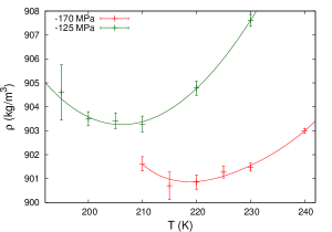
Figure 3: Detail of the densities for the -125 MPa (decreased by 0.8 Kg/m³) and -170 MPa isobars showing the existence of a density minimum. The error bars correspond to the 90% confidence interval calculated from the standard deviations obtained in the block procedure. Lines are a weighted fit of the data to a fourth order polynomial.

Despite the great computational effort and the notable accuracy of the density calculations, the uncertainty of the temperatures of minimum density is about 5 degrees and the loci of the TmD produce a less smooth curve than that of the TMD ones (see Fig. 2).

The existence of a density minimum in real water has not been described previously. Liu et al.Liu et al. (2007) have reported a density minimum in deeply supercooled confined deuterated water. At ambient pressure, the minimum density occurs at 210 K with a value of 1041 kg/m³. Despite that it is difficult to know how the confinement affects the water properties we may use this data as a rough guide of the behavior of bulk water. As to TIP4P/2005, previous simulation results indicated the existence of the density minimumPi et al. (2009); Russo and Tanaka (2014); Sumi and Sekino (2013) but the accuracy of the data did not allow for a trustworthy estimation of its value. The result of the present work at 0.1 MPa is $\rho$=938.1 kg/m³ and is located at 200$\pm$5 K. Assuming that the density of deuterated water is 1.106 times that of normal water,Liu et al. (2007) we get $\rho$=1038 kg/m³, close to the experimental result in confined water.

The difference between the temperature of maximum and minimum density has a peculiar behavior because it is larger near the retracing point of the TMD and decreases at both higher and lower pressures. At large negative pressures, the TMD and TmD lines converge asymptotically (point B in the bottom panel of Fig. 2). Below this pressure, the density no longer exhibits maxima nor minima.

As commented in the introduction, at the retracing point, the TMD curve must be crossed by the line joining the locus of isothermal compressibility extrema. The upper panel of Figure 4 shows $\kappa_{T}$ as a function of temperature for several isobars from -170 MPa to 100 MPa (for clarity only a few of the simulated isobars are depicted). For pressures higher than about -80 MPa the isobars show clearly the presence of a maximum and a minimum. At this pressure, the curve exhibits almost imperceptible extrema but, for a slightly lower pressure, the maximum and minimum of $\kappa_{T}$ collapse into an inflection point. Then, at large negative pressures, $\kappa_{T}$ is a a monotonously increasing function of temperature. The locus of $\kappa_{T}$ extrema are plotted, in the p-T plane, in the lower panel of Fig. 4 together with the TMD curve. As expected, both lines cross at the turning point of the TMD (point A in Fig. 4). Notice that the intersection point A lies near the pressure at which $\kappa_{T}$ becomes a monotonous function.

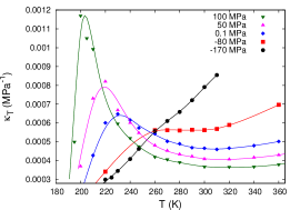
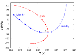
Figure 4: Top: Isothermal compressibility as a function of temperature along isobars. Bottom: locus of $\kappa_{T}$ extrema together with TMD line. Both curves intersect at the point A, the retracing point of the TMD. The curves are cubic splines to guide the eye.

On the other hand, theoretical considerationsPoole et al. (2005) indicate that the locus of isobaric heat capacity extrema along isotherms separates the TMD from the line of minimum densities, TmD. The simulation results for C_p along isotherms are presented in Figure 5 (upper panel). The isotherms show both a maximum and a minimum. The separation between these extrema becomes increasingly smaller as the temperature increases. Eventually, at a temperature slightly above 247 K, the maximum and minimum converge to an inflection point and C_p becomes a monotonous function. The pressures at which the C_p extrema occur for each isotherm are shown in the lower panel of Fig. 5. In this figure we have also depicted the locus of density extrema along isobars. As shown by Poole et al.,Poole et al. (2005) the latter curve must have a zero slope at the intersection point, a condition which is satisfactorily fulfilled by our simulations (see point B in Fig. 5). The location of this point for TIP4P/2005 is about (243 K, -203.4 MPa).

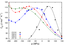
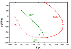
Figure 5: Top: Heat capacity at constant pressure along isotherms. Bottom: Locus of C_p extrema together with the curve of density extrema. Both lines intersect at point B separating the TMD and TmD. The curves are a guide to the eye.

It is clear at this point that the SLC conjecture is not valid for TIP4P/2005 and that the vapor-liquid (VL) spinodal should not meet the (retracing) TMD line. In the SF and LLCP scenarios both curves do not intersect. It is then interesting to check whether this is fulfilled by our calculations. We have tried to evaluate the VL spinodal by locating the zero slope of the pressure-volume curves along isotherms. The simulations were performed in the canonical (NVT) ensemble. However, the system with 4 000 molecules sometimes cavitated before providing statistically significant results. We were then forced to reduce the size of the system to 500 molecules. For these samples, the probability of a cavitation event is almost one order of magnitude smaller and it is then possible to obtain statistically significant results. It is well known that finite size effects may be important in this regionBinder (1992) so our calculations must be seen as a first approximation to the actual spinodal. The corresponding pressure-specific volume isotherms are presented in Figure 6 (top panel) from which we may extract the p-v-T values of the VL spinodal. It is to be noticed that the specific volume along the spinodal shows a non-monotonic dependence on both temperature and pressure (bottom panel of Fig.  6). As expected, the slope of the VL spinodal in the p-T plane is positive and do not meet the TMD curve (Figure 7).

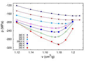
Figure 6: Estimation of the vapor-liquid spinodal. Top: Pressure as a function of the specific volume for several isotherms (asterisks indicate the position of the minimum). Bottom: Specific volume as a function of temperature along the vapor-liquid spinodal.

The results shown in the bottom panels of Figs. 4 and 5 together with the results of Fig. 6 allow us to give a comprehensive picture of the water anomalies and their relation to the vapor-liquid spinodal. The corresponding plot is presented in Figure 7. Notice that the lines of $\kappa_{T}$ and $C_{p}$ maxima approach one to another at high pressures and move away as the pressure decreases. In the SF scenario both curves would only converge at 0 K. Thus, although both the SF and LLCP scenarios are compatible with our results, the rate of convergence of these lines seem to favor the LLCP hypothesis. This conclusion is also supported by a comparison of Fig. 7 with the corresponding one for ST2.Poole et al. (2005) The scenarios of the ST2 and TIP4P/2005 water models are completely analogous and suggest that a critical point for TIP4P/2005 is very plausible. In fact, we have extended the lines of $\kappa_{T}$ and $C_{p}$ maxima up to the location of the LLCP proposed in recent papers.Yagasaki et al. (2014); Singh et al. (2016) The extended lines provide a smooth transition from the critical point to our simulation results for the response functions maxima.

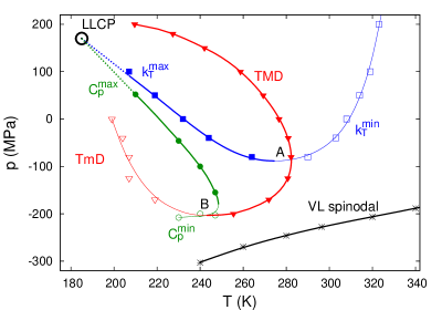
Figure 7: Comprehensive scenario relating thermodynamic water anomalies and the vapor-liquid spinodal. Dashed lines are an extension of the loci of $\kappa_{T}$ and $C_{p}$ maxima up to the proposed location of the LLCP.Yagasaki et al. (2014); Singh et al. (2016)

IV Concluding remarks

In this work we have calculated the loci of the extrema of several thermodynamic functions for the TIP4P/2005 water model. In particular, the maxima and minima of the isothermal compressibility along isobars and isobaric heat capacity along isotherms have been evaluated and put in connection with the maxima and minima of the density along isobars. Our work provides for the first time a comprehensive picture of the thermodynamic water anomalies for TIP4P/2005 and their relation to the vapor-liquid spinodal.

The interpretation of previous simulations for the TIP4P/2005 water model in the supercooled region has been rather controversial.Abascal and Vega (2010); Limmer and Chandler (2013); Overduin and Patey (2013); Yagasaki et al. (2014); Overduin and Patey (2015); Yagasaki et al. (2015) The debate has been mainly focussed on three issues: spontaneous phase separation, finite site effects and ice coarsening. Most of the calculations of this work correspond to the supercooled and/or the stretched regions though we have deliberately avoided the vicinity of the conjectured liquid-liquid region. Our results are then beyond the current debate on the possibility of observing spontaneous liquid-liquid phase separation.Yagasaki et al. (2014); Overduin and Patey (2015); Limmer and Chandler (2015); Yagasaki et al. (2015) This has allowed us to get converged results for the properties of interest with a large but affordable computational effort.

The size of the system, 4 000 water molecules, seems to ensure that our calculations are free of finite size effects. It has been reported that even larger samples could be needed for temperatures below the proposed LLCP.Overduin and Patey (2015) However, our calculations for the TMD indicate that the differences between the results obtained with 500 and 4 000 molecules are marginal (see Fig. 4 of supplemental material). Thus, at least at the thermodynamic conditions of this work, we do not observe a significant system size dependence.

It has been argued that the phenomenon suggesting metastability of two distinct liquid phases is actually coarsening of the ordered ice-like phase.Limmer and Chandler (2013) Again, the range of temperatures and pressures of this work indicate that our results are free of the problem of ice coarsening. In a recent study, Espinosa et al.Espinosa et al. (2014) have calculated the size of the critical cluster and the nucleation rate for the crystallization of TIP4P/2005 water as a function of the supercooling. The results for both magnitudes indicates beyond any doubt that our simulations correspond to a metastable liquid. Inherent to metastability is the formation and breaking of small clusters of the stable phase. Thus the question is not the appearance of small crystal nuclei but whether a critical cluster may appear in the simulation. Espinosa et al. have evaluated the supercooling required for the formation of a single critical cluster in a simulation with a box side of 40 Å (corresponding to a typical supercooled water density of about 0.94 g/cm$3$ in a system of 2 000 molecules) for 1 $\mu$s. At these conditions (very similar to those of our longest simulations) they report a 65 K supercooling. Since the melting temperature of the model is around 250 K, the appearance of a critical cluster above 185 K is a very unlikely event (notice that the lowest temperature of our calculations is 195 K).

Although in this work we have avoided the issue of the existence of a LLCP, it is evident that the overall picture is consistent with both the SF and LLCP conjectures. However, the way in which the lines of maximum $\kappa_{T}$ and $C_{p}$ approach one to another seem to indicate that they meet not too far from the region of calculations clearly favoring the LLCP hypothesis over the SF one. This idea is reinforced when one observes that the scenario presented in Fig 7 very much resembles that of ST2Poole et al. (2005) for which most authors give for demonstrating the existence of a LLCP.

It is important to stress that the significance of this work goes beyond the theoretical interpretation of simulation results. Most of the thermodynamic states relevant to this work corresponds to the negative pressures region where the water properties are largely unknown.Caupin and Stroock (2013) Since the TIP4P/2005 water model has demonstrated to provide semiquantitative predictions of the water properties in the supercooled and/or stretched regions,Abascal and Vega (2011); Pallares et al. (2014, 2016) the scenario of the water anomalies predicted by this model may provide a hint as to where the long-sought for extrema in response functions might become accessible to experiments.

Note added in proofs: After sending the accepted version of this work we have been aware of a paper by Lu et al.Lu et al. (2016) reporting a similar study using the coarse grained mW and mTIP4P/2005 water models.

V Supplemental materials for ”A comprehensive scenario of the thermodynamic anomalies of water using the TIP4P/2005 model”

V.1 Calculation of the uncertainty

The uncertainty has been calculated using a method proposed by HessHess (2002). The trajectory is divided in n_block blocks of length t_block and the average of the density for each block is calculated. The uncertainty of the total trajectory is then calculated as the standard deviation of the values of the n_block averages. Notice that these uncertainties are dependent of the number of blocks (or the block length). If t_block is very small, consecutive blocks are strongly correlated and the standard deviation does not represent the actual uncertainty of the total trajectory. As the block length increases, the correlation between blocks decreases so the uncertainty tends to an asymptotic value. However, for very large block length (or, more specifically, when n_block is low), the number of points to calculate the uncertainty is very reduced so the standard deviation shows a large statistical noise. In fact, well known statiscal considerations indicate that n_block should not be less than about 20.

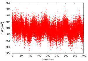
Figure 8: Densities along a 400 ns trajectory for the state point at T=200 K, p=-125 MPa.

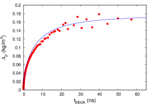
Figure 9: Uncertainties for the system of Fig. 8. Symbols are the standard deviations of the averages calculated in blocks of length t_block. The line is the standard deviation evaluated using a double exponential fit for the correlation between blocks.

The procedure of Ref. Hess, 2002 incorporates an important additional element, namely the calculation of the correlation between block averages and its fit to a double exponential. In this way, the discrete nature of the correlation between blocks is smoothed by the fit and the calculated uncertainties (eventually) lead to an asymptotic curve (for long enough trajectories). In summary, the procedure of Hess not only provides a reasonable evaluation of the uncertainty but also sheds light on the convergence of the trajectory. An example of the application of the method is presented in Figs. 9 and 10.

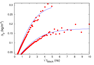
Figure 10: Block analysis of the uncertainties for the system of Fig. 8 as a function of the square root of the block length. The data correspond to the results for the full 400 ns trajectory (bottom) and for the first 100 ns (top). Notice that the number of blocks corresponding to the larger block length is only 4 in both cases. The analysis clearly indicates that a 100 ns trajectory is not long enough to obtain convergence.

V.2 Numerical values for the density at selected isobars

Table 1 presents the numerical values of the simulation results for the density of the TIP4P/2005 model along the isobars shown in Fig. 1 of the main paper.

Table 1: Densities of the TIP4P/2005 model along isobars

Temperature	Pressure	Density	Pressure	Density	Pressure	Density
(K)	(MPa)	(kg/m3)	(MPa)	(kg/m3)	(MPa)	(kg/m3)
195	0.1	939.3	-40	930.1	-80	922.9
200	0.1	938.4	-40	929.0	-80	921.7
205	0.1	939.6	-40	930.4	-80	920.7
210	0.1	945.4	-40	932.0	-80	921.9
220	0.1	957.5	-40	939.5	-80	925.7
230	0.1	972.85	-40	950.1	-80	932.0
240	0.1	984.77	-40	961.1	-80	940.35
247	0.1	990.68	-40	967.4	-80	-
260	0.1	997.24	-40	975.58	-80	953.99
270	0.1	999.38	-40	978.63	-80	957.48
280	0.1	999.66	-40	979.71	-80	958.89
290	0.1	998.48	-40	979.04	-80	958.39
300	0.1	996.19	-40	977.06	-80	956.43
310	0.1	992.95	-40	973.83	-80	953.13
320	0.1	988.77	-40	969.64	-80	948.62
340	0.1	978.36	-40	958.71	-80	-
360	0.1	965.52	-40	944.84	-80	921.07

V.3 Finite size effects on the TMD

Fig. 11 shows a comparison of the TMD line calculated using 500 (data taken from Ref. Pallares et al., 2016) and 4000 (this work) water molecules. The differences are quite small but systematic. Since the calculations were obtained using slightly different simulation parameters and also different version of GROMACS, it is very difficult to know whether the small departures are a consequence of the differences in the system size or in the simulation details.

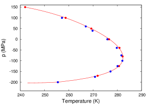
Figure 11: Locus of the maximum density temperatures for systems made of 500 (blue) and 4000 water molecules (red).

References

- Debenedetti (2003) P. G. Debenedetti, J. Phys. Condens. Matter 15, R1669 (2003).
- Speedy and Angell (1976) R. J. Speedy and C. A. Angell, J. Chem. Phys. 65, 851 (1976).
- Speedy (1982) R. J. Speedy, J. Phys. Chem. 86, 982 (1982).
- Poole et al. (1992) P. H. Poole, F. Sciortino, U. Essmann, and H. E. Stanley, Nature 360, 324 (1992).
- Sastry et al. (1996) S. Sastry, P. G. Debenedetti, F. Sciortino, and H. E. Stanley, Phys. Rev. E 53, 6144 (1996).
- Angell (2008) C. A. Angell, Science 319, 582 (2008).
- Sciortino et al. (1997) F. Sciortino, P. H. Poole, U. Essmann, and H. E. Stanley, Phys. Rev. E 55, 727 (1997).
- Xu et al. (2005) L. M. Xu, P. Kumar, S. V. Buldyrev, S. H. Chen, P. H. Poole, F. Sciortino, and H. E. Stanley, Proc. Nat. Acad. Sci. 102, 16558 (2005).
- Zanotti et al. (2005) J. M. Zanotti, M. C. Bellissent-Funel, and S.-H. Chen, Europhys. Lett. 71, 91 (2005).
- Mallamace et al. (2007) F. Mallamace, M. Broccio, C. Corsaro, A. Faraone, D. Majolino, V. Venuti, L. Liu, C.-Y. Mou, and S.-H. Chen, Proc. Nat. Acad. Sci. 104, 424 (2007).
- Mallamace et al. (2008) F. Mallamace, C. Corsaro, M. Broccio, C. Branca, N. González-Segredo, J. Spooren, S.-H. Chen, and H. E. Stanley, Proc. Nat. Acad. Sci. 105, 12725 (2008).
- Mishima and Stanley (1998a) O. Mishima and H. E. Stanley, Nature 396, 329 (1998a).
- Mishima and Stanley (1998b) O. Mishima and H. E. Stanley, Nature 392, 164 (1998b).
- Bellissent-Funel (1998) M. C. Bellissent-Funel, Europhys. Lett. 42, 161 (1998).
- Soper (2000) A. K. Soper, Chem. Phys. 258, 121 (2000).
- Mishima and Suzuki (2002) O. Mishima and Y. Suzuki, Nature 419, 599 (2002).
- Souda (2006) R. Souda, J. Chem. Phys. 125, 181103 (2006).
- Banerjee et al. (2009) D. Banerjee, S. N. Bhat, S. V. Bhat, and D. Leporini, Proc. Nat. Acad. Sci. 106, 11448 (2009).
- Taschin et al. (2013) A. Taschin, P. Bartolini, R. Eramo, R. Righini, and R. Torre, Nature Comm. 4, 2401 (2013).
- Pallares et al. (2014) G. Pallares, M. E. M. Azouzi, M. A. González, J. L. Aragonés, J. L. F. Abascal, C. Valeriani, and F. Caupin, Proc. Nat. Acad. Sci. 111, 7936 (2014).
- Sellberg et al. (2014) J. A. Sellberg, C. Huang, T. A. McQueen, N. D. Loh, H. Laksmono, D. Schlesinger, R. G. Sierra, D. Nordlund, C. Y. Hampton, D. Starodub, et al., Nature 510, 381 (2014).
- Seidl et al. (2015) M. Seidl, A. Fayter, J. N. Stern, G. Zifferer, and T. Loerting, Phys. Rev. B 91, 144201 (2015).
- Caupin (2015) F. Caupin, J. Non Cryst. Sol. 407, 441 (2015).
- Debenedetti and D’Antonio (1986) P. G. Debenedetti and M. C. D’Antonio, J. Chem. Phys. 84, 3339 (1986).
- Pallares et al. (2016) G. Pallares, M. A. Gonzalez, J. L. F. Abascal, C. Valeriani, and F. Caupin, Phys. Chem. Chem. Phys. 18, 5896 (2016).
- Stillinger and Rahman (1974) F. H. Stillinger and A. Rahman, J. Chem. Phys. 60, 1545 (1974).
- Poole et al. (1993) P. H. Poole, F. Sciortino, U. Essmann, and H. E. Stanley, Phys. Rev. E 48, 3799 (1993).
- Brovchenko et al. (2005) I. Brovchenko, A. Geiger, and A. Oleinikova, J. Chem. Phys. 123, 044515 (2005).
- Liu et al. (2009) Y. Liu, A. Z. Panagiotopoulos, and P. G. Debenedetti, J. Chem. Phys. 131, 104508 (2009).
- Sciortino et al. (2011) F. Sciortino, I. Saika-Voivod, and P. H. Poole, Phys. Chem. Chem. Phys. 13, 19759 (2011).
- Liu et al. (2012) Y. Liu, J. C. Palmer, A. Z. Panagiotopoulos, and P. G. Debenedetti, J. Chem. Phys. 137, 214505 (2012).
- Kesselring et al. (2012) T. A. Kesselring, G. Franzese, S. V. Buldyrev, H. J. Herrmann, and H. E. Stanley, Sci. Rep. 2, 474 (2012).
- Poole et al. (2013) P. H. Poole, R. K. Bowles, I. Saika-Voivod, and F. Sciortino, J. Chem. Phys. 138, 034505 (2013).
- Palmer et al. (2013) J. C. Palmer, R. Car, and P. G. Debenedetti, Faraday Discuss. 167, 77 (2013).
- Palmer et al. (2014) J. C. Palmer, F. Martelli, Y. Liu, R. Car, A. Z. Panagiotopoulos, and P. G. Debenedetti, Nature 510, 385 (2014).
- Yagasaki et al. (2014) T. Yagasaki, M. Matsumoto, and H. Tanaka, Phys. Rev. E 89, 020301 (2014).
- Palmer et al. (2016) J. C. Palmer, F. Martelli, Y. Liu, R. Car, A. Z. Panagiotopoulos, and P. G. Debenedetti, Nature 531, E2 (2016).
- Limmer and Chandler (2011) D. T. Limmer and D. Chandler, J. Chem. Phys. 135, 134503 (2011).
- Chandler (2016) D. Chandler, Nature 531, E1 (2016).
- Berendsen et al. (1987) H. J. C. Berendsen, J. R. Grigera, and T. P. Straatsma, J. Phys. Chem. 91, 6269 (1987).
- Vega and Abascal (2011) C. Vega and J. L. F. Abascal, Phys. Chem. Chem. Phys 13, 19663 (2011).
- Pi et al. (2009) H. L. Pi, J. L. Aragonés, C. Vega, E. G. Noya, J. L. F. Abascal, M. A. González, and C. McBride, Molec. Phys. 107, 365 (2009).
- Mahoney and Jorgensen (2000) M. W. Mahoney and W. L. Jorgensen, J. Chem. Phys. 112, 8910 (2000).
- Rick (2004) S. W. Rick, J. Chem. Phys. 120, 6085 (2004).
- Yamada et al. (2002) M. Yamada, S. Mossa, H. E. Stanley, and F. Sciortino, Phys. Rev. Lett. 88, 195701 (2002).
- Paschek (2005) D. Paschek, Phys. Rev. Lett. 94, 217802 (2005).
- Vega et al. (2005) C. Vega, E. Sanz, and J. L. F. Abascal, J. Chem. Phys. 122, 114507 (2005).
- Abascal and Vega (2007a) J. L. F. Abascal and C. Vega, Phys. Chem. Chem. Phys 9, 2775 (2007a).
- Abascal and Vega (2007b) J. L. F. Abascal and C. Vega, J. Phys. Chem. C 111, 15811 (2007b).
- Horn et al. (2004) H. W. Horn, W. C. Swope, J. W. Pitera, J. D. Madura, T. J. Dick, G. L. Hura, and T. Head-Gordon, J. Chem. Phys. 120, 9665 (2004).
- Abascal et al. (2005) J. L. F. Abascal, E. Sanz, R. García Fernández, and C. Vega, J. Chem. Phys. 122, 234511 (2005).
- Abascal and Vega (2005) J. L. F. Abascal and C. Vega, J. Chem. Phys. 123, 234505 (2005).
- Vega et al. (2009) C. Vega, J. L. F. Abascal, M. M. Conde, and J. L. Aragones, Faraday Discuss. 141, 251 (2009).
- Abascal and Vega (2011) J. L. F. Abascal and C. Vega, J. Chem. Phys. 134, 186101 (2011).
- Abascal and Vega (2010) J. L. F. Abascal and C. Vega, J. Chem. Phys. 133, 234502 (2010).
- Sumi and Sekino (2013) T. Sumi and H. Sekino, RSC Adv. 3, 12743 (2013).
- Limmer and Chandler (2013) D. T. Limmer and D. Chandler, J. Chem. Phys. 138, 214504 (2013).
- Overduin and Patey (2013) S. D. Overduin and G. N. Patey, J. Chem. Phys. 138, 184502 (2013).
- Bresme et al. (2014) F. Bresme, J. W. Biddle, J. V. Sengers, and M. A. Anisimov, J. Chem. Phys. 140, 161104 (2014).
- Russo and Tanaka (2014) J. Russo and H. Tanaka, Nature Comm. 5, 3556 (2014).
- Overduin and Patey (2015) S. D. Overduin and G. N. Patey, J. Chem. Phys. 143, 094504 (2015).
- Singh et al. (2016) R. S. Singh, J. W. Biddle, P. G. Debenedetti, and M. A. Anisimov, J. Chem. Phys. 144, 144504 (2016).
- van der Spoel et al. (2005) D. van der Spoel, E. Lindahl, B. Hess, G. Groenhof, A. E. Mark, and H. J. C. Berendsen, J. Comput. Chem. 26, 1701 (2005).
- Hess et al. (2008) B. Hess, C. Kutzner, D. van der Spoel, and E. Lindahl, J. Chem. Theory Comput. 4, 435 (2008).
- Essmann et al. (1995) U. Essmann, L. Perera, M. L. Berkowitz, T. Darden, H. Lee, and L. G. Pedersen, J. Chem. Phys. 103, 8577 (1995).
- Hess et al. (1997) B. Hess, H. Bekker, H. J. C. Berendsen, and J. G. E. M. Fraaije, J. Comput. Chem. 18, 1463 (1997).
- Hess (2008) B. Hess, J. Chem. Theory Comput. 4, 116 (2008).
- Nosé (1984) S. Nosé, Mol. Phys. 52, 255 (1984).
- Hoover (1985) W. G. Hoover, Phys. Rev. A 31, 1695 (1985).
- Parrinello and Rahman (1981) M. Parrinello and A. Rahman, J. Appl. Phys. 52, 7182 (1981).
- Hess (2002) B. Hess, J. Chem. Phys. 116, 209 (2002).
- (72) See supplementary material at http://dx.doi.org/10.1063/1.4960185 for a detailed report of the estimate of the uncertainties, the numerical values of the densities at selected isobars, and an analysis of finite size effects on the tmd.
- Angell and Kanno (1976) C. A. Angell and H. Kanno, Science 193, 1121 (1976).
- Agarwal et al. (2011) M. Agarwal, M. P. Alam, and C. Chakravarty, J. Phys. Chem. B 115, 6935 (2011).
- Liu et al. (2007) D.-Z. Liu, Y. Zhang, C.-C. Chen, C.-Y. Mou, P. H. Poole, and S.-H. Chen, Proc. Nat. Acad. Sci. 104, 9570 (2007).
- Poole et al. (2005) P. H. Poole, I. Saika-Voivod, and F. Sciortino, J. Phys. Condens. Matter 17, L431 (2005).
- Binder (1992) K. Binder, in Computational Methods in Field Theory, edited by H. Gausterer and C. B. Lang (Springer-Verlag, Berlin-Heidelberg, 1992), pp. 59–125.
- Yagasaki et al. (2015) T. Yagasaki, M. Matsumoto, and H. Tanaka, Phys. Rev. E 91, 016302 (2015).
- Limmer and Chandler (2015) D. T. Limmer and D. Chandler, Phys. Rev. E 91, 016301 (2015).
- Espinosa et al. (2014) J. R. Espinosa, E. Sanz, C. Valeriani, and C. Vega, J. Chem. Phys. 141, 18C529 (2014).
- Caupin and Stroock (2013) F. Caupin and A. D. Stroock, in Liquid polymorphism, edited by H. E. Stanley (John Wiley and Sons Inc., NJ, 2013), vol. 152 of Adv. Chem. Phys., pp. 51–80.
- Lu et al. (2016) J. Lu, C. Chakravarty, and V. Molinero, J. Chem. Phys. 144, 234507 (2016).

References

- Hess (2002) B. Hess, J. Chem. Phys. 116, 209 (2002).
- Pallares et al. (2016) G. Pallares, M. A. Gonzalez, J. L. F. Abascal, C. Valeriani, and F. Caupin, Phys. Chem. Chem. Phys. 18, 5896 (2016).