Light WIMP searches involving electron scattering

Abstract

We consider light WIMP searches involving the detection of recoiling electrons.

Abstract

In the present work we examine the possibility for detecting electrons in dark matter searches. These detectors are considered to be the most appropriate for detecting light dark matter particles with a mas in the MeV region. We analyze theoretically some key issues involved in such a detection and we perform calculations for the expected rates employing reasonable theoretical models.

I Introduction

The combined MAXIMA-1 Hanary et al. (2000); Wu et al. (2001); Santos et al. (2002), BOOMERANG Mauskopf et al. (2002); Mosi et al. (2002) DASI Halverson et al. (2002) and COBE/DMR Cosmic Microwave Background (CMB) observations Smoot et al. (1992) imply that the Universe is flat Jaffe et al. (2001) and that most of the matter in the universe is dark Spergel et al. (2003), i.e. exotic. These results have been confirmed and improved by the recent WMAP Spergel et al. (2007) and Planck Pla data. Combining the data of these quite precise measurements one finds:

$$\Omega_{b}=0.0456\pm 0.0015,\,\Omega_{\mbox{{\tiny CDM}}}=0.228\pm 0.013\mbox{ and }\Omega_{\Lambda}=0.726\pm 0.015~{}$$

(the more recent Planck data yield a slightly different combination $\Omega_{\mbox{{\tiny CDM}}}=0.274\pm 0.020,\quad\Omega_{\Lambda}=0.686\pm 0.020)$. It is worth mentioning that both the WMAP and the Plank observations yield essentially the same value of $\Omega_{m}h^{2}$, but they differ in the value of $h$, namely $h=0.704\pm 0.013$ (WMAP) and $h=0.673\pm 0.012$ (Planck). Since any “invisible” non exotic component cannot possibly exceed $40\%$ of the above $\Omega_{\mbox{{\tiny CDM}}}$  Bennett et al. (1995), exotic (non baryonic) matter is required and there is room for cold dark matter candidates or WIMPs (Weakly Interacting Massive Particles).
Even though there exists firm indirect evidence for a halo of dark matter in galaxies from the observed rotational curves, see e.g. the review Ullio and Kamioknowski (2001), it is essential to directly detect such matter in order to unravel the nature of the constituents of dark matter.

The possibility of such detection, however, depends on the nature of the dark matter constituents and their interactions.

The WIMPs are expected to have a velocity distribution with an average velocity which is close to the rotational velocity $\upsilon_{0}$ of the sun around the galaxy, i.e. they are completely non relativistic. In fact a Maxwell-Boltzmann leads to a maximum energy transfer which is close to the average WIMP kinetic energy $\prec T\succ\approx 0.4\times 10^{-6}mc^{2}$. Thus for GeV WIMPS this average is in the keV regime, not high enough to excite the nucleus, but sufficient to measure the nuclear recoil energy. For light dark matter particles in the MeV region, which we will also call WIMPs, the average energy that can be transferred is in the few eV region. So this light WIMPs can be detected by measuring the electron recoil after the collision. Electrons may of course be produced by heavy WIMPS after they collide with a heavy target which results in a shake up of the atom yielding ”primordial” electron production Vergados and Ejiri (2004); Ejiri et al. (2006); Moustakidis et al. (2005). This approach for sufficiently heavy WIMPs and target nuclei can produce electrons energies even in the 30 keV region, with a spectrum very different from that arising after a direct WIMP-electron collision. Furthermore WIMP-electron collisions involving WIMPs with masses in the few GeV region have also recently appeared Roberts et al. (2016a)-Roberts et al. (2016b). In the present work, however, we will restrict ourselves in the case of light WIMPs with a mass in the region of the electron mass.

We will draw from the experience involving WIMPs in the GeV region. The event rate for such a process can be computed from the following ingredients Lewin and Smith (1996):

• The elementary electron cross section. In this case we will consider the case of a scalar WIMP, whose mass, as far as we know has not been constrained by any experiment, but it leads to mass dependent cross section favoring light particles. This scalar WIMP couples with ordinary Higgs with a quartic coupling, the properties of which are being actively determined by the LHC experiments. Thus the WIMP interacts with electrons via Higgs exchange with an amplitude proportional to the electron $fm_{e}$.

• The knowledge of the WIMP particle density in our vicinity. This is extracted from WIMP density in the neighborhood of the solar system, obtained from the rotation curves measurements. The number density of these MeV WIMPs, however, is expected to be six orders of magnitude bigger than that of the standard WIMPs due to the smaller WIMP mass involved.

• The WIMP velocity distribution. In the present work we will consider a Maxwell-Boltzmann (MB) distribution.

In the electron recoil experiments, like the nuclear measurements first proposed more than 30 years ago Goodman and Witten (1985), one has to face the problem that the process of interest does not have a characteristic feature to distinguish it from the background. So since low counting rates are expected the background is a formidable problem. Some special features of the WIMP- interaction can be exploited to reduce the background problems, such as the modulation effect: This yields a periodic signal due to the motion of the earth around the sun. Unfortunately this effect, also proposed a long time ago Drukier et al. (1986) and subsequently studied by many authors Primack et al. (1988); Gabutti and Schmiemann (1993); Bernabei (1995); Lewin and Smith (1996); Abriola et al. (1999); Hasenbalg (1998); Vergados (2003); Green (2003); Savage et al. (2006); FKL , is small in the case of nuclear recoils, but we expect to be a bit larger in the case of the electron recoils. There has always been an interest in light WIMPs, see e.g. the recent work Essig et al. (2012a). In fact the first direct detection limits on sub-GeV dark matter from XENON10 have recently been obtained Essig et al. (2012b). This is encouraging, but based on our experience with standard nuclear recoil experiments to excited states Vergados et al. (2013), one has to make sure that the proper kinematics has to be used in dealing with bound electrons. Clearly the binding electron energy plays a similar role as the excitation energy of the nucleus, in determining the small fraction of the WIMP’s energy to be transferred to the recoiling system. It is therefore clear that Light WIMPs are quite different in energy, mass, interacting particle, and flux. Accordingly one needs detectors capable of detecting low energy light WIMPs in the midst of formidable backgrounds, i.e. detectors which are completely different from current WIMP detectors employed for heavy WIMP searches.

In the present paper we will address the implications of light scalar WIMPs on the expected event rates scattered off electrons. The interest in such a WIMP has recently been revived due to a new scenario of dark matter production in bounce cosmology Li et al. (2014); Cheung et al. (2014) in which the authors point out the possibility of using dark matter as a probe of a big bounce at the early stage of cosmic evolution. A model independent study of dark matter production in the contraction and expansion phases of the Big Bounce reveals a new venue for achieving the observed relic abundance in which dark matter was produced completely out of chemical equilibriumCheung and Vergados (2015) . In this way, this alternative route of dark matter production in bounce cosmology can be used to test the bounce cosmos hypothesis Cheung and Vergados (2015).

In any case, regardless of the validity of the big bounce universe scenario, the scalar WIMPs have the characteristic feature that the elementary cross section in their scattering off ordinary quarks or electrons is increasing as the WIMPs get lighter, which leads to an interesting experimental feature, namely it is expected to enhance the event rates at low WIMP mass. In the present calculation we will adopt this view and study its implications in direct dark matter searches compared to other types of WIMPs, such as the neutralinos, which we will call standard WIMPs.

Scalar WIMP’s can occur in particle models. Examples are i) In Kaluza-Klein theories for models involving universal extra dimensions (for applications to direct dark matter detection see, e.g., Oikonomou et al. (2007)). In such models the scalar WIMPs are characterized by ordinary couplings, but they are expected to be quite massive, ii) extremely light particles  Boehm and Fayet (2004), which are not relevant to the ongoing WIMP searches, iii) Scalar WIMPS such as those considered previously in various extensions of the standard model Ma (2006), which can be quite light and long lived protected by a discrete symmetry. Thus they are viable cold dark matter candidates.

II The particle model

The WIMP is assumed to be a scalar particle $\chi$ interacting with another scalar $\phi$ via a quartic coupling as discussed, e.g. in refs Silveira and Zee (1985); Holz and Zee (201); Bento et al. (2001, 2000), and more recently in Ref. Cheung and Vergados (2015). In fact the quartic coupling

$$\phi+\phi\rightarrow\chi+\chi$$ (1)

involving the scalar WIMP $\chi$ and the Higgs $\phi$ leads to a Feynman diagram shown in Fig. 1(a) and results to a mass dependent nucleon cross section Cheung and Vergados (2015) of the form:

$$\sigma_{p}=\sigma_{0}(p)\frac{1}{\left(1+m_{\chi}/m_{p}\right)^{2}},$$ (2)

where $\sigma_{0}(p)$ depends on the quartic coupling $\lambda$ and the quark structure of the nucleon. We will assume in this work that $\phi$ is the Higgs scalar discovered at LHC and the quartic coupling entering our model is the same with that involving the Higgs as has been determined by the LHC experiments.

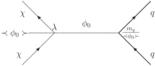
(a)

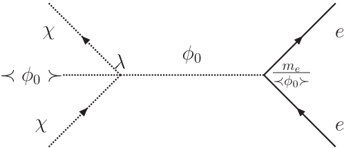
(b)

Figure 1: (a) The quark - scalar WIMP scattering mediated by a scalar particle. Note that the amplitude is independent of the vacuum expectation value $\prec\phi_{0}\succ$ of the scalar. (b) The corresponding diagram for electron-scalar WIMP scattering.

$\sigma_{e}\rightarrow$pb

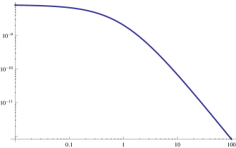
(a)

$\sigma_{e}\rightarrow$pb

(b)

Figure 2: The WIMP-electron cross section in pb as a function of WIMP mass, in units of the electron mass, as obtained our model in the case the WIMP is a scalar particle with the value of $\lambda$ extracted from the Higgs LHC data (a) and that extracted from the nucleon cross section limit of $\sigma_{p}=10^{-8}$pb obtained from the exclusion plots of XENON100 at 50 GeV Aprile et al. (2012) (b).

$\frac{m_{\chi}}{m_{e}}\rightarrow$

In the case of light WIMPs with mass less than 100 MeV one cannot produce a detectable recoiling nucleus, but electrons Moustakidis et al. (2005) could be produced with energies in the eV region, which, in principle, could be detected with current mixed phase detectors  Aprile et al. (2014). If the WIMP is a scalar particle, it can interact with electrons via the Feynman diagram shown in Fig. 1(b).

For WIMPs with mass in the range of the electron mass, both the WIMP and the electron are not relativistic. So the expression for elementary electron cross section is similar to that of hadrons , i.e. it is now given by:

$$\sigma_{e}=\frac{1}{4\pi}\frac{\lambda^{2}m_{e}^{2}}{m_{\phi}^{4}}\left(\frac{m_{e}m_{\chi}}{m_{e}+m_{\chi}}\right)^{2}\frac{1}{m_{\chi}^{2}}=\sigma_{0}(e)\frac{1}{\left(1+m_{\chi}/m_{e}\right)^{2}}$$ (3)

with $\sigma_{0}(e)$ determined by the Higgs particle discovered at LHC, namely $\lambda=1/2$, $m_{\phi}=126$ GeV. One finds:

$$\sigma_{0}(e)=\frac{1}{4\pi}\frac{\lambda^{2}m_{e}^{2}}{m_{\phi}^{4}}\approx 8.0\times 10^{-9}\mbox{pb},$$ (4)

This is a respectable size cross section, which depends on the ratio $m_{\chi}/m_{e}$. Alternatively one could fix $\sigma_{0}$ by using the nucleon cross limit Cheung and Vergados (2015) extracted from experiments, e.g. $\sigma_{p}=10^{-8}$ pb from XENON100 Aprile et al. (2012, 2011), which leads to $\sigma_{0}(p)=5.0\times 10^{-5}$ pb. We thus find

$$\sigma_{0}(e)=\sigma_{0}(p)\frac{m^{2}_{e}}{m_{p}^{2}}\approx 1.3\times 10^{-11}\mbox{ pb},$$ (5)

which, if true, would imply a much smaller value for $\lambda$.

Anyway we will treat the value of $\sigma_{0}(e)$ as a parameter, which may be fixed if and when the experimental data become available. The obtained cross section is exhibited in Fig. 2b. We note that this mass dependence of the cross section of scalar WIMPs results in a suppression of the cross section in the high WIMP mass regime. In what follows we will write $\sigma_{0}$ but it is understood that we mean $\sigma_{0}(e)$.

Before proceeding further with evaluation of the event rates in the case of light WIMPs it is instructive to review the experimental hurdles that must overcome to make their detection feasible.

III Experimental aspects

So far, we have discussed mainly some theoretical aspects of light WIMPs in the MeV region and have presented theoretical calculations of the expected light WIMP signals. Here we briefly discuss experimental aspects of light WIMP searches, which are very different compared with those of heavy WIMP searches.

Light WIMPs are quite different in energy, mass, interacting particle, and flux. Accordingly one needs detectors which are completely different from current WIMP detectors for heavy WIMPs. Detectors are required to observe low-energy light WIMP signals beyond/among BG signals to identify the light WIMPs. Experimental aspects to be considered for light WIMP detectors are: i) the particle to be detected, ii) the event rate, iii) the signal pulse height, iv) the background rate and v) the detector threshold energy. We will now examine each of these items.

• Particle to be detected.
  Light WIMPs are detected by observing a recoil/scattered electron in the continuum region. In case that the WIMP interaction produces an ion-electron pair, one can detect the ion and/or the electron, and/or photons associated with the ion-electron pair. If the recoil electron or the ion-electron pair energy is absorbed by the detector, one may measure the temperature change. These are similar to those from heavy WIMPs except that their energies are very different. It is noted that atomic bound electrons are not excited by the light WIMPs with $E\leq$ a few eV.

• Event rate.
  The cross section of $\sigma_{0}\approx 8.2\times 10^{-9}$ pb is an order of magnitude larger than the present XENON limit of $\sigma_{0}\approx$ 10^-9 pb for heavy WIMPs Aprile et al. (2012). The flux rate is around $n\approx 1.3\times 10^{10}$cm^-2s^-1, which is larger by a factor of 50 GeV/0.5 MeV$\approx 10^{5}$ . Then the event rate for Xe detector is around $R\approx 1.8\times 10^{3}$ /(t.y), which is an order of magnitude larger than the present limit for 50 GeV heavy WIMPs Aprile et al. (2012).

• Signal pulse height.
  The electron signal energy for light WIMPs is around 0.5-1 eV. This energy is 4 orders of magnitude smaller than the Xe nuclear recoil energy of around 25 keV for the 50 GeV WIMP. The nuclear recoil signal is quenched by a factor 2-20, depending on the atomic number, in most heavy WIMP detectors. Thus the actual signal height for the light WIMP is 3 orders of magnitude smaller than that for the heavy WIMP.

• Background rate
  There are three types of background origins for WIMP detectors, radioactive (RI) impurities, neutrons associated with cosmic rays, and electric noises. $\beta-\gamma$ rays from RI impurities produce BG electron signals, which are similar to electron signals from light WIMPs as well as as those encountered in the case of double $\beta$ decay detectors, which measure $\beta$ rays. BG rate for a typical future DBD (double $\beta$ decay ) detectors is around 1/(t y keV) =10^-3/(t y eV) at a few MeV region ab (1). Then one may expect a similar BG rate in the eV region. This is 3 orders of magnitude smaller than the signal rate. Neutrons do not contribute to BGs in light WIMP detectors, although nuclear recoils from neutron nuclear reactions are most serious BGs for heavy WIMP detectors.

  Electric noises are most serious for light WIMP detectors because of the very low energy signals. The nuclear recoil energy from heavy WIMPs is typically a few 10 keV, and the signal pulse height is around a few keV if they are quenched, depending on the detector. This is of the same order of magnitude as electric noise levels. Thus one can search for heavy WIMPs by measuring the higher velocity component above the electric noises On the other hand, the signal height for light WIMP is far below that of typical electric noises for current heavy WIMP detector.

• Energy threshold
  The energy threshold $E_{th}$ for WIMP detectors is set necessarily below the WIMP signal, but just above the electric noise to be free from the noise. Then a very low energy threshold of an order of sub eV is required for light WIMP searches. This is 3-4 orders of magnitude smaller than the level around 1-3 keV for most heavy WIMP detectors Aprile et al. (2012) and Agnose et al. (2013). Germanium semiconductor detectors are widely used to study low energy neutrinos and WIMPs. The ionization energy is 0.67 eV. Thus it can be used in principle for energetic light WIMPs. In practice, their threshold of around 200 eV Chen (2014) or more is still far above the light WIMP signals. Bolometers are, in principle, low energy threshold and high energy resolution detectors, but the energy threshold of practical 10 kg-scale bolometers are orders of magnitude higher than the light WIMP signal. Thus light WIMP detectors are necessarily different types from the present heavy WIMP detectors.

  It is indeed a challenge to develop light WIMP detectors with low-threshold energy of the order of eV. Since the event rate is as large as 2 10³/t y, one can use a small volume detector of the order of 10 kgr at low temperature. In general, electric noises are random in time. Then, coincidence measurements of two signals are quite effective to reduce electric noise signals in case that one light WIMP produces 2 or more signals. One possible detector would be an ionization- scintillation detector, where one light WIMP interaction produces one ionized ion and one electron. In case that the ionized ion traps an electron nearby and emits a scintillation photon, one may measure the primary electron in coincidence with the scintillation photon. Nuclear emulsion may be of potential interest for low energy electrons. We briefly discuss possible new detection methods in section VII.

IV The differential WIMP-electron rate

The evaluation of the rate proceeds as in the case of the standard WIMP-nucleon scattering, but we will give the essential ingredients here to establish notation. We will begin by examining the case of a free electron.

IV.1 Free electrons

Since both the WIMP and the electron are not relativistic one finds that the momentum transferred to the electron ${\bf q}$ has a magnitude is given by

$$q=2\mu_{r}\upsilon\xi,\,\mu_{r}=\frac{m_{\chi}m_{e}}{m_{e}+m_{\chi}}\mbox{=WIMP-electron reduced mass},\upsilon=\mbox{ WIMP velocity},\,\xi=\hat{\upsilon}.\hat{q}$$

The differential cross section is now given by :

$$d\sigma=\sigma_{0}\frac{\mu_{r}^{2}}{m_{\chi}^{2}}2\xi d\xi,\,0\leq\xi\leq 1$$ (6)

From this, after integrating over $\xi$, we obtain the total cross as given by Eq. 3.
The energy transfer is given by

$$T=\frac{q^{2}}{2m_{e}}=\frac{2\mu_{r}^{2}\upsilon^{2}\xi^{2}}{m_{e}}$$ (7)

From this relation we find that the fraction of the energy of the WIMP transferred to the electron, when taking $\left<\xi^{2}\right>=1/3$ for scattering at forward angles, is

$$\frac{T}{T_{\chi}}=\frac{4}{3}\frac{x}{(1+x)^{2}},\,x=\frac{m_{e}}{m_{\chi}}$$ (8)

This situation is exhibited in Fig. 3.

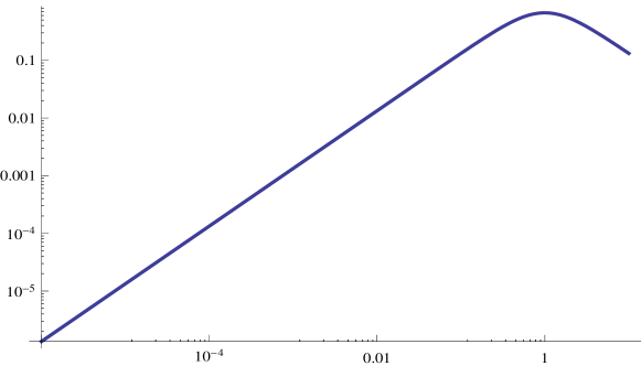
$\rightarrow x=\frac{m_{\chi}}{m_{e}}$

Figure 3: The fraction of the WIMP energy transferred to the electron as a function of $x=\frac{m_{\chi}}{m_{e}}$

We thus see that this fraction attains a maximum when $x=1$, i.e., when the two masses are equal. Away from this value it becomes smaller. The effect is more crucial for very light WIMPs, since their average energy is much smaller.

We also find from Eq. (7) that the average energy of the electron is given by

$$\left<T\right>=\frac{2}{3(1+x)^{2}}\left<\beta^{2}\right>m_{e}c^{2},\left<\beta^{2}\right>=\prec\left(\frac{\upsilon}{c}\right)^{2}\succ=0.8\times 10^{-6}$$ (9)

Thus for MeV WIMPs the average energy transfer is in the eV region, which is reminiscent of the standard WIMPs where GeV mass leads to an energy transfer in the keV region. The maximum energy transfer corresponds to the escape velocity which is $\upsilon_{esc}\approx 2\sqrt{\left<\upsilon^{2}\right>}$, which leads to a value four times higher. The exact expression of the maximum electron energy will be given below.

It is preferable to rewrite Eq. 6 in terms of the energy of the recoiling electron T and the WIMP velocity using the relation given by Eq. (7). We thus find

$$d\sigma=\sigma_{0}\frac{1}{2\upsilon^{2}}\frac{m_{e}}{m_{\chi^{2}}}dT$$ (10)

We also find that

$$\upsilon=\sqrt{\frac{m_{e}T}{2\mu^{2}_{r}\xi^{2}}}\rightarrow\upsilon\geq\sqrt{\frac{m_{e}T}{2\mu^{2}_{r}}}\rightarrow\upsilon_{min}=\sqrt{\frac{m_{e}T}{2\mu^{2}_{r}}}$$ (11)

In other words the minimum velocity consistent with the energy transfer $T$ and the WIMP mass is constrained as above. The maximum velocity allowed is determined by the velocity distribution and it will be indicated by $\upsilon_{esc}$. From this we can obtain the differential rate per electron in a given velocity volume $\upsilon^{2}d\upsilon d\Omega$ as follows:

$$dR=\frac{\rho_{\chi}}{m_{\chi}}\upsilon\sigma_{0}\frac{1}{2}\frac{m_{e}}{m_{\chi^{2}}}dTf({\mbox{\boldmath$\upsilon$}})d\upsilon d\Omega$$ (12)

where $f({\mbox{\boldmath$\upsilon$}})$ is the velocity distribution of WIMPs in the laboratory frame. Integrating over the allowed velocity distributions we obtain:

$$dR=\frac{\rho_{\chi}}{m_{\chi}}\sigma_{0}\frac{1}{2}\frac{m_{e}}{m^{2}_{\chi}}dT\eta(\upsilon_{\mbox{\tiny{min}}}),\,\eta(\upsilon_{\mbox{\tiny{min}}})=\int_{\upsilon_{\mbox{\tiny{min}}}}^{\upsilon_{esc}}f({\mbox{\boldmath$\upsilon$}})\upsilon d\upsilon d\Omega$$ (13)

$\eta(\upsilon_{\mbox{\tiny{min}}})$ is a crucial parameter.
Before proceeding further we find it convenient to express the velocities in units of the Sun’s velocity. We should also take note of the fact the velocity distribution is given with respect to the center of the galaxy. For a M-B distribution this takes the form:

$$\frac{1}{\pi\sqrt{\pi}}e^{-y^{{}^{\prime}2}},\,y^{{}^{\prime}}=\frac{\upsilon^{{}^{\prime}}}{\upsilon_{0}},\,\upsilon_{0}=220\mbox{ km/s}$$ (14)

We must transform it to the local coordinate system :

$${\bf y}^{{}^{\prime}}\rightarrow{\bf y}+{\hat{\upsilon}}_{s}+\delta\left(\sin{\alpha}{\hat{x}}-\cos{\alpha}\cos{\gamma}{\hat{y}}+\cos{\alpha}\sin{\gamma}{\hat{\upsilon}}_{s}\right),\,\delta=\frac{\upsilon_{E}}{\upsilon_{0}}$$ (15)

with $\gamma\approx\pi/6$, ${\hat{\upsilon}}_{s}$ a unit vector in the Sun’s direction of motion, $\hat{x}$ a unit vector radially out of the galaxy in our position and $\hat{y}={\hat{\upsilon}}_{s}\times\hat{x}$. The last term in parenthesis in Eq. (15) corresponds to the motion of the Earth around the Sun with $\upsilon_{E}\approx 28$ km/s being the modulus of the Earth’s velocity around the Sun and $\alpha$ the phase of the Earth ($\alpha=0$ around June 3rd). The above formula assumes that the motion of both the Sun around the Galaxy and of the Earth around the Sun are uniformly circular. Since $\delta$ is small, we can expand the distribution in powers of $\delta$ keeping terms up to linear in $\delta$. Then Eq. 13 can be cast in the form

$$dR=\left(\frac{\rho_{\chi}}{m_{\chi}}{\upsilon_{0}}\right)\sigma_{0}\frac{m_{t}Z_{eff}}{Am_{p}}1.9\times 10^{6}\frac{1}{2}\frac{m_{e}}{m_{\chi^{2}}}dT\left(\Psi_{0}(y_{min})+\Psi_{1}(y_{min})\cos{\alpha}\right),$$ (16)

where, in the above equation, the first term in parenthesis represents the average flux of WIMPs, the second provides the scale of the elementary cross section (in the present model the elementary cross section contains an additional mass dependence), the third term gives the number of electrons available for the scattering in a target of mass $m_{t}$ containing atoms with mass number $A$ and active electrons $Z_{eff}$ and the fourth is essentially the inverse of the square of the Sun’s velocity in units of $c$ (its origin has its root in Eq. 10). Furthermore for a M-B distribution one finds:

$$\Psi_{0}(x)=\frac{1}{2}H\left(y_{esc}-x\right)\left[\mbox{erf}(1-x)+\mbox{erf}(x+1)+\mbox{erfc}(1-y_{\mbox{\tiny{esc}}})+\mbox{erfc}(y_{\mbox{\tiny{esc}}}+1)-2\right]$$ (17)

and

$$\Psi_{1}(x) = \frac{1}{2}H\left(y_{esc}-x\right)\delta\left[\frac{-\mbox{erf}(1-x)-\mbox{erf}(x+1)-\mbox{erfc}(1-y_{\mbox{\tiny{esc}}})-\mbox{erfc}(y_{\mbox{\tiny{esc}}}+1)}{2}\right.$$ (18)

$$\left.+\frac{e^{-(x-1)^{2}}}{\sqrt{\pi}}+\frac{e^{-(x+1)^{2}}}{\sqrt{\pi}}-\frac{e^{-(y_{\mbox{\tiny{esc}}}-1)^{2}}}{\sqrt{\pi}}-\frac{e^{-(y_{\mbox{\tiny{esc}}}+1)^{2}}}{\sqrt{\pi}}+1\right],$$

with

$$y_{min}=\frac{\upsilon_{min}}{\upsilon_{0}}=\frac{1}{\upsilon_{0}}\sqrt{\frac{m_{e}T}{2\mu^{2}_{r}}},\,y_{esc}=\frac{\upsilon_{esc}}{\upsilon_{0}}$$

In the above expression the Heaviside function $H$ guarantees that the required kinematical condition is satisfied. One can factor the constants out in the above equation to get

$$\frac{dR}{d(T/1\mbox{eV})}=\Lambda\left(\Sigma_{0}\left(\frac{m_{\chi}}{m_{e}},\frac{T}{1\mbox{eV}}\right)+\Sigma_{1}\left(\frac{m_{\chi}}{m_{e}},\frac{T}{1\mbox{eV}}\right)\cos{\alpha}\right)$$ (19)

where

$$\Sigma_{i}(t,s)=\frac{1}{t^{3}}\Psi_{i}\left(1.23\left(1+\frac{1}{t}\right)\sqrt{s}\right),\,i=0,1$$ (20)

and

$$\Lambda=1.4\frac{\rho_{\chi}}{m_{e}}{\upsilon_{0}}\sigma_{0}\frac{m_{t}Z_{eff}}{Am_{p}}.$$ (21)

The meaning of $Z_{eff}$ will become clear after we consider the fact that the electrons are not free but bound in the atom. Thus they are not all available for scattering, i.e. $Z_{eff}<Z$ . We will now estimate $\Lambda$ considering the following input:

• the elementary cross section $\sigma_{0}=8.2\times 10^{-9}pb=8.2\times 10^{-45}\mbox{cm}^{2}$

• The total cross cross section, in units of $\sigma_{0}$, e.g. $\sigma_{av}$ =0.2 for a WIMP mass about the electron mass (see below).

• The particle density of WIMPs in our vicinity:

  $$n=0.3\times 10^{3}\mbox{(MeV /cm}^{3}\mbox{)/0.511MeV}\approx 600\mbox{cm}^{-3}$$

  (we use the electron mass in this estimate. The correct mass dependence has been included in evaluating $\sigma_{av}$). This value leads to a flux:

  $$n\times 220\mbox{ km/s}=1.3\times 10^{10}\mbox{cm}^{-2}\mbox{s}^{-1}$$

• The number of electrons in a Kg of Xe:

  $$\left(1/(131\times 1.67\times^{-27})\right)Z_{eff}=4.6\times 10^{24}Z_{eff}$$

Taking $Z_{eff}=54$, i.e. all electrons in Xe participating, we expect about

$$\approx 0.5\mbox{ events per kg.y}.$$

Encouraged by this estimate, even though it has been obtained with a much smaller elementary cross section than previous estimates Essig et al. (2012a), we are going to proceed in evaluating the expected spectrum of the recoiling electrons.

We first show the behavior of the the generic function $\Psi_{0}$ as a function of the electron energy for various WIMP masses (see Fig. 4).

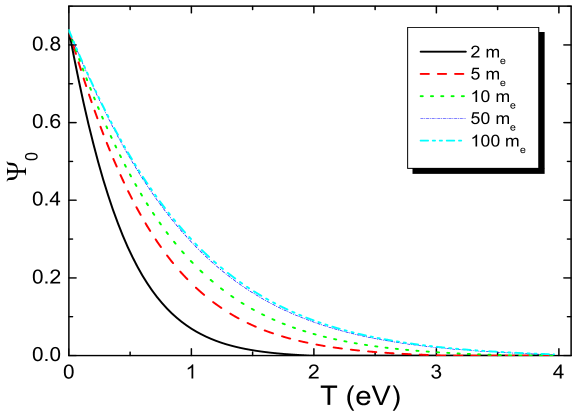
Figure 4: The shape of the differential cross section, as described by the function $\Psi_{0}$, as a function of the electron recoil in eV for the WIMP masses $(2,5.,10,50,100)m_{e}$. The electrons are assumed to be free. As in the case of WIMPs the specrum does not exhibit any special structure.

In the case of the modulation amplitude we get the picture of Fig. 5. We observe that the pattern is analogous to that found in the case of nuclear recoils.

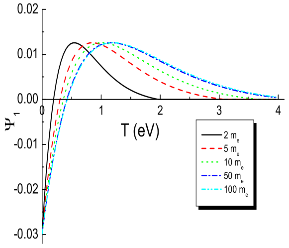
Figure 5: The same as in Fig. 4 for the modulated amplitude described by the function $\Psi_{1}$, as a function of the electron energy $T$ in eV.

The function $\Sigma_{0}(t,s)$ is exhibited in Fig. 6.

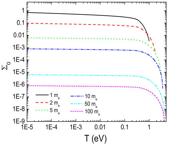
Figure 6: The shape of the differential cross section as a function of the electron energy $T$ in eV for the WIMP masses $(1,2,5.,10,50,100)m_{e}$. The electrons are assumed to be free. The WIMP masses are indicated as in Fig. 4. The spectrum does not exhibit any special structure.

The various atomic physics approximations involved involved involving relatively high electron, as e.g in recent works Roberts et al. (2016a)-Roberts et al. (2016b), are not important in our case.The obtained rate, however, can increase substantially, if we include the correction of the outgoing electron wave due to the coulomb field. In beta decays this is done via the simple Fermi function Venkataramaiah et al. (1985):

$$F(k,Z,\eta,\gamma)=\left(kR\right)^{2\gamma-2}e^{\pi\nu}\left|\frac{\Gamma(\gamma+i\eta)}{\Gamma(2\gamma)}\right|^{2}|M(\gamma+i\eta,2\gamma,2ikr)|^{2},$$ (22)

where

$$\gamma=\sqrt{1-\alpha^{2}Z^{2}},\,\eta=\alpha Z\frac{\sqrt{k^{2}+m^{2}c^{2}}}{k}=Z\alpha\frac{T+m_{e}c^{2}}{\sqrt{T^{2}+2m_{e}c^{2}T}}$$ (23)

and $M(\gamma+i\eta,2\gamma,2ikr)$ is the Coulomb function represented by a confluent hypergeometric function. For $|(\gamma+i\eta)2ikr|<<2\gamma$, which is the case for momenta and $r$ encountered in beta decay, the coulomb function becomes unity. This is not true in our case. Furthermore the first momentum dependent function, employed in the standard nuclear decay, is different in our case, since the electron is not produced at the origin, but it is ejected from an atomic orbit, i.e., $r$ is of the order in Bohr orbit. The coulomb wave function for large values of $\eta$ depends on the variable $2\eta kr=2\alpha_{Z}m_{e}R\approx 2\alpha_{Z}m_{e}\bar{r}(n,Z,\gamma)$, where $\bar{r}(n,Z,\gamma)$ is the average radius, i.e it becomes essentially independent of the energy $T$. It can be shown that Lan ${\bar{r}}(n,Z,\gamma)=\frac{1}{2}\left(3n^{2}-(\gamma-1)\gamma)\right)\frac{1}{m_{e}\alpha Z}$. Thus $2\eta kr\approx\left(3n^{2}-(\gamma-1)\gamma\right)$, i.e.

$$M(\gamma+i\eta,2\gamma,2ikr) \rightarrow\Gamma(2\gamma)f_{c}(\gamma,n),$$

$$f_{c}(\gamma,n) \approx \frac{2}{\sqrt{\pi}}\left(\sqrt{\left(3n^{2}-(\gamma-1)\gamma\right)}\right)^{-2\gamma+1/2}j_{2\gamma-1/2}\left(2\sqrt{\left(3n^{2}-(\gamma-1)\gamma\right)}\right)$$ (24)

where $j_{2\gamma-1/2}(y)$ is the spherical Bessel function. Furthermore to a good approximation :

$$e^{\pi\nu}|\Gamma(\gamma+i\eta)|^{2}\approx\frac{2\pi\eta}{1-e^{-2\pi\eta}}$$

(see, e.g., Landau’s book Lan ). Thus one finds the Fermi function

$$F(T,Z,n,\eta,\gamma)\approx\left(\sqrt{T^{2}+2m_{e}T}\bar{r}(n,Z,\gamma)\right)^{2\gamma-2}f^{2}_{c}(\gamma,n)\frac{2\pi\eta}{1-e^{-2\pi\eta}}.$$ (25)

This function, which depends on the electron energy as well as the atomic parameters $n$ and $Z$ may lead to an enhancement for low energy electrons, see Fig. 7. For a given $Z$, $F$ depends on $n$ and thus a suitable average $n$ should perhaps be employed for a given target. Anyway the effect of the Fermi function has not been included in Fig. 6.

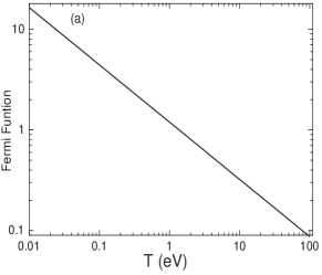
(a)

(b)

Figure 7: The Fermi function $F$ as a function of the electron recoil energy for $n=3$ and $Z=50$ (a) and $n=4$ and $Z=60$ (b) .

Integrating the differential rate given by Eq. (19) over the electron spectrum we obtain the total rate:

$$R=\Lambda\left(\sigma_{av}+\sigma_{td}\cos{\alpha}\right)$$ (26)

where $\sigma_{av}$ and $\sigma_{td}\cos{\alpha}$ are the average and time dependent (modulated) cross sections respectively in units of $\sigma_{0}$, i.e. of the elementary cross section. The obtained quantity $\sigma_{av}$ is shown in Fig. 8 for free electrons both without the Fermi function as well as with the Fermi function for two values $n$ and $Z$, $n$ assumed to be sort of average. We see that the effect on the total cross section is large. Thus we find that the cross sections (in units of $\sigma_{0}$, for a WIMP with the mass of the electron we get values 0.2, 0.8 and 2.2 for cases (a), (b) and (c) respectively (see Fig. 8), while for $n=2$ and $Z=50$ we find 0.3. In our estimates we will adopt an average enhancement factor of 8 due to the Fermi function.

(a)

(b)

(c)

Figure 8: The total average WIMP-electron cross section in units $\sigma_{0}$ as a function of the WIMP mass in eV. In panel (a) the Fermi function was neglected, while in panels (b) and (c) the Fermi function $F$ for $n=3$ and $Z=50$ and $n=4$ and $Z=60$ respectively has been employed.

Taking into account the Fermi function the above estimate becomes 4.0 events/(kg.y).

V Effects of binding of electrons

The binding of the electrons comes in in two ways. The first the most obvious. A portion of the energy of the WIMP will not go to recoil, but it will be spent to release the bound electron. The second comes from the fact that the initial electron is not at rest but it has a momentum distribution, which is the Fourier transform of its wave function in coordinate space. We will first concentrate on the effect on the kinematics of the binding energy.

V.1 The effect of the momentum distribution

sectionThe effect of the momentum distribution In this case of bound electrons the phase space reads:

$$J=\frac{1}{(2\pi)^{2}}\int d^{3}{\bf p}\left|\tilde{\phi}_{n\ell}({\bf p})\right|^{2}d^{3}{\bf q}d^{3}{\bf p}_{\chi}^{{}^{\prime}}\delta\left({\bf p}+{\bf p}_{\chi}-{\bf p}_{\chi}^{{}^{\prime}}-{\bf q}\right)\delta\left(\frac{{\bf p}^{2}_{\chi}}{2m_{\chi}}-\frac{{\bf p}^{{}^{\prime}2}_{\chi}}{2m_{\chi}}-\frac{{\bf q}^{2}}{2m_{e}^{2}}-b\right)$$ (27)

where $\tilde{\phi}_{n\ell}(p)$ is the electron wf in momentum space. After the integration over the momentum ${\bf p}$ via the $\delta$ function we obtain:

$$J=\frac{1}{(2\pi)^{2}}\int\left|\tilde{\phi}_{n\ell}({\bf p^{\prime}_{\chi}}-{\bf p_{\chi}}+{\bf q})\right|^{2}d^{3}{\bf p}_{\chi}^{{}^{\prime}}d^{3}{\bf q}\delta\left(\frac{{\bf p}^{2}_{\chi}}{2m_{\chi}}-\frac{{\bf p}^{{}^{\prime}2}_{\chi}}{2m_{\chi}}-\frac{{\bf q}^{2}}{2m_{e}^{2}}-b\right)$$ (28)

The integration over the magnitude of ${\bf p^{\prime}_{\chi}}$ can be done using the energy conserving $\delta$ function and we obtain

$$J=\frac{1}{(2\pi)^{2}}\int d^{3}{\bf q}Q^{2}d\Omega_{{\bf Q}}\left|\tilde{\phi}_{n\ell}\left({\bf Q}-{\bf p_{\chi}}+{\bf q}\right)\right|^{2}\frac{m_{\chi}}{Q},\,{\bf Q}=\hat{e}\sqrt{\left(m_{\chi}\upsilon\right)^{2}-q^{2}x-2m_{\chi}b}$$ (29)

with x=$m_{\chi}/m_{e}$ and $\hat{e}$ a unit vector in the direction of ${\bf p^{\prime}_{\chi}}$. We thus find the important constraint:

$$\upsilon>\upsilon_{\mbox{\tiny min}},\,\upsilon_{\mbox{\tiny min}}=\frac{\sqrt{q^{2}x+2m_{\chi}b}}{m_{\chi}}\mbox{ or }\upsilon_{\mbox{\tiny min}}=\sqrt{\frac{2}{m_{\chi}}}\sqrt{T+b}$$ (30)

This already sets a limit on the range of the variables $b$ and $T$ of interest to experiments.

V.2 Range of $b$ and $T$

Regarding $b$ the above conditions imply:

$$(T)_{\mbox{\tiny{max}}}=\frac{1}{2}m_{\chi}\upsilon^{2}_{\mbox{\tiny{esc}}}-b,\,b_{\mbox{\tiny{max}}}=\frac{1}{2}m_{\chi}\upsilon^{2}_{\mbox{\tiny{esc}}}$$

where $b_{\mbox{\tiny{max}}}$ is associated with with zero maximum recoil energy and is exhibited as a function of WIMP mass in Fig. 9

$b\rightarrow$ eV

$m_{\chi}\rightarrow\frac{m_{\chi}}{m_{e}}$

Figure 9: The maximum binding electron energy $b_{\mbox{\tiny{max}}}$ in eV as a function of $\frac{m_{\chi}}{m_{e}}$ accessible to WIMP-electron scattering.

What seriously affects detecting light WIMPs in the presence of large binding energies is the minimum WIMP velocity required to eject an electron. One finds that in order to surpass the barrier of a given binding energy $b$ the WIMP must have a minimum velocity at most $v_{\mbox{\tiny{esc}}}$ and a high mass, even if the electron energy is zero. This the minimum $x=m_{\chi}/m_{e}$ required for this purpose is exhibited in Fig. 10b(a). The actual value of $x=m_{\chi}/m_{e}$ must, of course, be larger to get a reasonable rate.

$\left(\frac{m_{\chi}}{m_{e}}\right)_{\mbox{\tiny{min}}}\rightarrow$

(a)

$b\rightarrow$ eV

$T_{\mbox{\tiny{max}}}\rightarrow$ eV

(b)

Figure 10: The minimum $\frac{m_{\chi}}{m_{e}}$ required to eject an electron with binding energy b in eV (a). The maximum outgoing electron energy $T_{\mbox{\tiny{max}}}$ as a function of $x=\frac{m_{\chi}}{m_{e}}$ for various binding energies $b$ (b) . In this panel the graphs correspond to $b=$1, 2, 5 and 10 eV from left to right.

$\rightarrow x=\frac{m_{\chi}}{m_{e}}$

Finally we present in Fig. 10b(b) the maximum possible energy for outgoing electrons as a function of the WIMP mass for various binding energies.

V.3 the phase space integral

To proceed further we must evaluate the above integral we must select a suitable coordinate system, e.g. one with the $z$-axis along the initial WIMP velocity, the $x$ axis in the direction of the outgoing WIMP and as $y$ axis perpendicular to the the plane of the other two. Then we find

$$J = \frac{1}{(2\pi)}\int d^{3}{\bf q}m_{\chi}{Q}\int d\xi_{1}d\phi$$ (31)

$$\left|\tilde{\phi}_{n\ell}\left(\sqrt{\left|Q^{2}+(m_{\chi}\upsilon)^{2}+q^{2}-2qm_{\chi}\upsilon\xi-2m_{\chi}\upsilon Q\xi_{1}+2qQ\left(\xi\xi_{1}+\sqrt{1-\xi^{2}}\sqrt{1-\xi_{1}^{2}}\cos{\phi}\right)\right|}\right)Y^{\ell}_{m}(\hat{\omega})\right|^{2}$$

where $\hat{\omega}$ is a unit vector in the direction of ${\bf Q}-{\bf p_{\chi}}+{\bf q}$.
There is no hope for obtaining an analytic expression with further approximations. We set $\cos{\phi}=0$ expecting that its contribution of this term will average out to zero. The remaining integral is still complicated but for $s$ states we we find

$$J=\frac{1}{(2\pi)}\int d^{3}{\bf q}m_{\chi}{Q}\int_{-1}^{1}d\xi_{1}\left|\tilde{\phi}_{n\ell}\left(Q^{2}+(m_{\chi}\upsilon)^{2}+q^{2}-2m_{\chi}q\upsilon\xi-2m_{\chi}Q\upsilon\xi_{1}+2qQ\xi\xi_{1}\right)\right|^{2}$$ (32)

We now have to consider two cases:

• $q\xi\neq y$. Setting now

  $$z=\frac{\sqrt{Q^{2}+(m_{\chi}\upsilon)^{2}+q^{2}-2m_{\chi}q\upsilon\xi-2m_{\chi}Q\upsilon\xi_{1}+2qQ\xi\xi_{1}}}{p_{0}(nZ}$$

  where $p_{0}(n,Z)=(\alpha Z)/n)m_{e}$ the scale of momentum of the bound electron wave function and $z$ dimensionless we obtain

  $$J=\frac{1}{(2\pi)}\int d^{3}{\bf q}m_{\chi}{Q}\frac{p^{2}_{0}(n,Z)}{Q(q\xi-m_{\chi}\upsilon)}\frac{1}{p_{0}^{3}(n,Z)}\int_{\eta_{+}}^{\eta_{-}}zdz\left|\tilde{\phi}_{n\ell}(z)\right|^{2}$$ (33)

  with $\int z^{2}dz\Omega\left|\tilde{\phi}_{n\ell}({\bf z})\right|^{2}$ normalized to one and

  $$\eta_{\pm}=\frac{\sqrt{Q^{2}+q^{2}+(m_{\chi}\upsilon)^{2}-2m_{\chi}q\upsilon\xi\pm 2Q(q\xi-m_{\chi}\upsilon)}}{p_{0}(n,Z)}$$

  The integral over $z$ can be done analytically for $s$ states. Thus

  $$J=\frac{1}{(2\pi)}\int d^{3}{\bf q}\frac{1}{p_{0}(n,Z)}\psi_{1}(\xi,q,\upsilon,b,p_{0}(n),\,\psi_{1}(\xi,q,\upsilon,b,p_{0}(n,Z))=\frac{m_{\chi}}{(q\xi-m_{\chi}\upsilon)}\int_{\eta_{+}}^{\eta_{-}}zdz\left|\tilde{\phi}_{n\ell}(z)\right|^{2}$$ (34)

  Integrating over the angular part of ${\bf q}$ we obtain :

  $$dJ=\frac{q}{p_{0}(n,Z)}qdq\psi_{2}(q,\upsilon,b,p_{0}(n,Z)),\,\psi_{2}(q,\upsilon,b,p_{0}(n,Z))=\int_{-1}^{1}d\xi\psi_{1}(\xi,q,\upsilon,b,p_{0}(n,Z))$$ (35)

• $q\xi=y$. Then

  $$dJ=\frac{m_{\chi}Q}{yp_{0}(n,Z)}qdq\psi^{\prime}_{2}(q,\upsilon,b,p_{0}(n,Z)),\,\psi^{\prime}_{2}(q,\upsilon,b,p_{0}(n,Z))$$ (36)

  with

  $$\psi^{\prime}_{2}(q,\upsilon,b,p_{0}(n,Z))=\int_{(Q^{2}+(y-q)^{2})/p^{2}_{0}(n,Z)}^{(Q^{2}+(y+q)^{2})/p^{2}_{0}(n,Z)}zdz\left|\tilde{\phi}_{n\ell}(z)\right|^{2}$$ (37)

  This situation does not occur in practice.

The above lead to a cross section:

$$d\sigma=\frac{1}{\upsilon}|{\cal A}|^{2}dJ$$ (38)

where ${\cal A}$ is the invariant amplitude for the process. In the case of scalar WIMPs we have:

$$|{\cal A}|^{2}=\frac{(\lambda m_{e})^{2}}{m_{H}^{4}}\frac{1}{(2m_{\chi})^{2}},$$ (39)

where the last factor comes from the normalization of the scalar field. By setting

$$\frac{(\lambda m_{e})^{2}}{m_{H}^{4}}=4\pi\sigma_{0}$$

we find

$$d\sigma=\sigma_{0}\frac{1}{\upsilon}\frac{\pi}{m_{\chi}^{2}}dJ$$ (40)

One can cast Eq. (40) in a form similar to the expression for free electrons, namely

$$d\sigma=\sigma_{0}\frac{1}{2\upsilon^{2}}\frac{m_{e}}{m_{\chi^{2}}}dT$$ (41)

$$d\sigma=\sigma_{0}\frac{1}{\upsilon^{2}}\frac{m_{e}}{m_{\chi}^{2}}dT\tilde{\Lambda}(T,\upsilon,b,p_{0}(n,Z)),\,\tilde{\Lambda}(T,\upsilon,b,p_{0}(n,Z))=2\pi\upsilon\frac{\sqrt{2m_{e}T}}{p_{0}(n,Z)}\psi_{2}(\sqrt{2m_{e}T},\upsilon,b,p_{0}(n,Z))$$ (42)

In order to get the differential rate one must fold the above expression with the velocity distribution $f(\mbox{\boldmath$\upsilon$})$

$$\frac{dR}{dT}\propto\sigma_{0}\frac{m_{e}}{m_{\chi}^{2}}\left[\int_{\sqrt{2(b+T)/m_{\chi}}}^{\upsilon_{\mbox{\tiny{esc}}}}\tilde{\Lambda}(T,\upsilon,b,p_{0}(n,Z))f(\mbox{\boldmath$\upsilon$})\upsilon d\upsilon d\hat{\mbox{\boldmath$\upsilon$}}\right]$$ (43)

Note the appearance of the quantities $b$ and $\tilde{\Lambda}$ as a result of the electron binding. The behavior of the function $\tilde{\Lambda}$ as a function of the velocity and its numerical value will significantly affect the obtained rates. In order to obtain it the remaining integrals must be done numerically for each electron orbit separately , which is not trivial. This is currently under study, but at present will report results obtained in an approximate scheme valid for relatively low mass WIMPs, which is adequate for our purposes.

V.4 A convenient approximation for light WIMPs

As we have said in the case of scalar WIMPs the cross section is suppressed for WIMPs much heavier than the electron. In this case the momentum of the outgoing electron is small compared to the $p_{0}(n,Z)$. Let us assume that:

$$\frac{Q(m_{\chi\upsilon})}{p^{2}_{0}(n,Z)}<1$$

This means that

$$x^{2}\upsilon\sqrt{\upsilon-\upsilon_{1}}\leq\alpha^{2},\,\upsilon_{1}=\sqrt{2(b+T)/xm_{e}}\leq\upsilon_{\mbox{\tiny esc}}$$

This quantity as small so long as

$$x<\frac{(\alpha Z)}{\upsilon_{\mbox{\tiny esc}}}=1.2Z\approx 50\mbox{ for a large atom }$$

For such values of $x$ we can expand the integral $\int_{\eta_{+}}^{\eta_{-}}zdz\left|\tilde{\phi}_{n\ell}(z)\right|^{2}$ up to second order in the small parameter. The result, e.g. for $1s$ hydrogenic wave functions, is:

$$J_{1}=\frac{16Q(m_{\chi}\upsilon-q\xi)}{\pi^{2}p^{2}_{0}(n,Z)}$$

Integrating over the angles of the outgoing electron we obtain

$$dJ=q^{2}dq\frac{64Q^{2}m_{\chi}m_{\chi}\upsilon}{\pi p^{5}_{0}(n,Z)}$$ (44)

Proceeding as above we obtain

$$\tilde{\Lambda}=\tilde{\Lambda}_{0}(Z)\sqrt{\frac{2T}{m_{e}}}\frac{x^{4}}{(\alpha Z)^{5}}\upsilon^{2}(\upsilon^{2}-\upsilon_{1}^{2})$$ (45)

or

$$\tilde{\Lambda}=\tilde{\Lambda}_{0}(Z)x^{4}\sqrt{T}y^{2}\left(y^{2}-\frac{6.59(b+T)}{x}\right),\,\tilde{\Lambda}_{0}(1)=3.5\times 10^{-3}$$ (46)

where $b$ and $T$ are in eV and $y$ is the WIMP velocity in units of the sun’s velocity. A similar expression with a slightly different constant $\tilde{\Lambda}_{0}(Z)$ is expected to hold for other electron orbitals.

This function must be multiplied with the velocity distribution before proceeding with the needed integrations to obtain the rate. We exhibit the thus resulting distribution of velocity for various values of $x,b,T$ in Figs 11- 14.

$f(\frac{\upsilon}{\upsilon_{0}})\rightarrow$

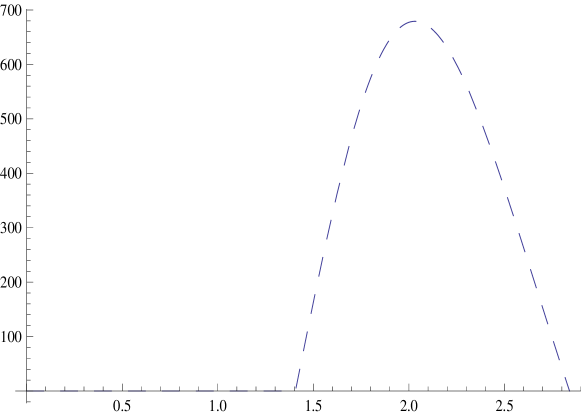
$\rightarrow\frac{\upsilon}{\upsilon_{0}}$

Figure 11: The velocity distribution obtaine with $x=2$ and $b=T=1$ eV. Note the lower bound on the velocity to the binding of the electrons.

$f(\frac{\upsilon}{\upsilon_{0}})\rightarrow$

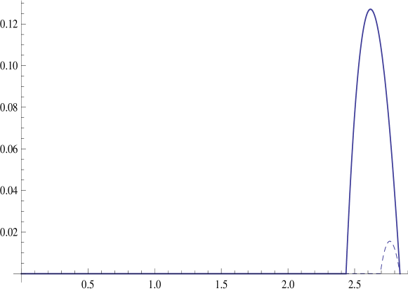
$\rightarrow\frac{\upsilon}{\upsilon_{0}}$

Figure 12: The velocity distribution obtained with $x=5$, $T=2$eV and $b=2.5$ and 3.5 eV associated with the solid and dashed line respectively. Note the large effect of the binding both on the scale and the velocity range for so light WIMPs.

$f(\frac{\upsilon}{\upsilon_{0}})\rightarrow$

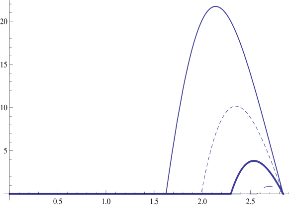
$\rightarrow\frac{\upsilon}{\upsilon_{0}}$

Figure 13: The velocity distribution obtained with $x=10$. We have selected $T=2$eV and $b=2,4$ and 6 eV associated with the solid dashed, and thick solid line respectively. Note the increase in the scale but the restriction in the velocity range (the $b$=8 eV is barely seen).

$f(\frac{\upsilon}{\upsilon_{0}})\rightarrow$

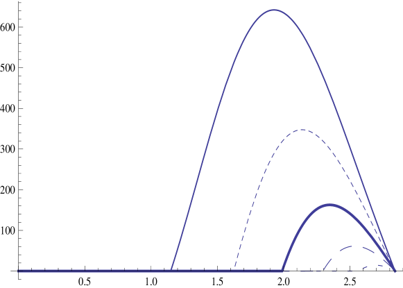
$\rightarrow\frac{\upsilon}{\upsilon_{0}}$

Figure 14: The velocity distribution obtained with $x=20$. Now we have selected $T=2$eV and $b=2,6,10,14$ and 18 eV corresponding to the solid, dashed, thick solid and long dashed lines respectively. Note the large increase in the scale but the restriction in the velocity range (the $b$=18 eV is barely seen).

VI Some results for bound electrons

We will limit ourselves to $b\geq 1$ eV and $x\leq 100$ After integrating with the velocity distribution we obtain the electron spectra shown in Figs 15- 17b

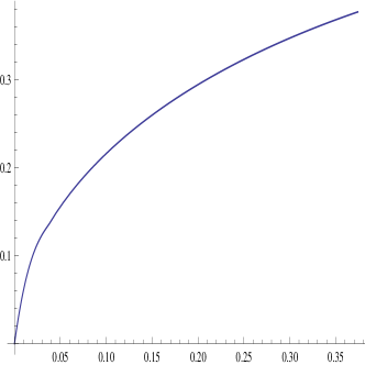
$\rightarrow T$ eV .

Figure 15: The electron spectrum for bound electrons corresponding $x=1$. Only electrons with $b<1$ eV can be ejected

$\Sigma_{0}\rightarrow$

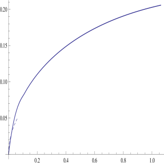
(a)

$\Sigma_{0}\rightarrow$

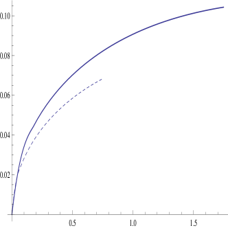
(b)

Figure 16: The same as in Fig. 15, but for $x=10$ in panel (a) and $x=20$ in panel (b). In both cases only electrons with $b<3$ eV can be ejected. Notice, however, that the spectrum is suppressed for $b=2$ (dotted line) compared to the corresponding one for $b=1$ (solid line)

$\rightarrow T$ eV .

$\Sigma_{0}\rightarrow$

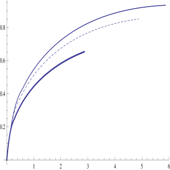
(a)

$\Sigma_{0}\rightarrow$

(b)

Figure 17: The same as in Fig. 16b, but for $x=50$ in panel (a) and $x=100$ in panel (b). In panel (a) the spectrum is shown for $b=1,\,2$ and 4 eV. In panel (b) the spectra for $b=1,\,2,\,4$ and 8 eV are shown with $b$ increasing downwards. The curve corresponding to $b=10$ is not visible.

$\rightarrow T$ eV

After integrating over the energy spectrum we obtain the cross section $\sigma_{av}$ in units of $\sigma_{0}$ shown in Fig. 18 as a function of the WIMP mass for various binding energies. It is perhaps better to show $\sigma_{av}$ as a function of the binding energy. For $x=10$ only $b\leq 1$ are available. For $b=1$ we find $\sigma_{av}=0.1$ in units of $\sigma_{0}$. For larger $x$, $\sigma_{av}$ is exhibited in Fig. 19b.

$\frac{\sigma_{av}}{\sigma_{0}}\rightarrow$

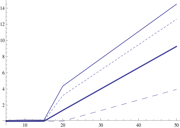
$\rightarrow x=\frac{m_{\chi}}{m_{e}}$

Figure 18: The cross section $\sigma_{av}$ in units of $\sigma_{0}$ as a function of $x=\frac{m_{\chi}}{m_{e}}$ for binding energies $b=$1, 2, 4, and 8 eV increasing downwards (the curve for $b=10$ is not visible).

$\frac{\sigma_{av}}{\sigma_{0}}\rightarrow$

(a)

$\frac{\sigma_{av}}{\sigma_{0}}\rightarrow$

(b)

Figure 19: The cross section $\sigma_{av}$ in units of $\sigma_{0}$ as a function of $b$ in eV for $x=\frac{m_{\chi}}{m_{e}}=$15 (dotted line) and 20 (solid line) (a) and for $x=\frac{m_{\chi}}{m_{e}}=$50 and 100 (b) (the lower curve corresponds to the smaller $x$).

$\rightarrow b$ eV

We thus see that using hydrogenic wave functions we find that, for $m_{\chi}$ greater $10m_{e}$, electrons with $b<15$ eV become available. The number of electrons with relatively small binding energy for some targets of interest are shown in table 1.

Table 1: The number of electrons with binding energies less than $b_{\rm upb}$ for a given set of targets.

Target	$b_{\rm upb}=5$ eV	$b_{\rm upb}=10$ eV	$b_{\rm upb}=15$ eV	$b_{\rm upb}=20$ eV	$b_{\rm upb}=30$ eV
9F	-	-	-	5	5
11Na	1	1	1	1	1
32Ge	4	4	4	4	14
52Te	4	4	6	6	6
53I	5	5	7	7	7
54Xe	-	-	6	6	8
83Bi	3	5	5	5	15

Anyway there seem to be which leads $Z_{eff}=5$ for a suitable atom with large $Z$. Thus for $Z_{eff}=5$ one can conservatively $\sigma_{av}$ to be $\approx 0.15$, which leads to about 1 event per kg-y compared to the 3 per kg-y we got above for lighter WIMPs without the electron binding. The Fermi function is incorporated into the results.

VII discussion

We have seen that the use of electron detectors may be a good way to directly detect light WIMPs in the MeV region. The electron density in our vicinity is very high, the elementary WIMP-electron cross section section may be quite large and the event rate may be further enhanced by the behavior of the Fermi function at low energies. With bound atomic electrons, however, there seems to be a problem, because a small fraction of electrons, $Z_{eff}/Z$, can be exploited, with $Z_{eff}$ being those electrons with binding energies below the 15 eV range. This is reminiscent of the difficulty encountered in the inelastic WIMP nucleus scattering, whereby only very low excited states can be reached. We have seen that the expected rates for low energy electron recoils due to light WIMPs are sensitive to the Fermi function corrections. In fact the inclusion of such corrections may increase the rate by factors of 8 for low energy electrons. So event rates of about 1 to 3 events per kg-y are possible.

It has recently been suggested that it is possible to detect even very light WIMPS, much lighter than the electron, utilizing Fermi-degenerate materials like superconductorsHPZ . In this case the energy required is essentially the gap energy of about $1.5kT_{c}$, which is in the meV region, i.e the electrons are essentially free. The authors are perhaps aware of the fact that not all the kinetic energy of the WIMP can be transferred to the system. As we have seen the maximum fraction is approximately 1/3 and occurs if the mass of the WIMP is equal to $m_{e}$, see Eq. (8) for $x=1$. These authors probably have a way to circumvent the fact that a small amount of energy will be deposited, partly because a small fraction of energy of the WIMP will be transferred to their system (see Fig. 3) and also because the average energy of the WIMP is smaller. Anyway, if they manage to accumulate a large number of electrons in their targets, the obtained rates maybe sufficient. More recently it is claimed that even smaller energies in meV can be detected in the case of Liquid Helium Schutz and Zurec (2016). The expected event rates and the total energy deposited in such essentially bolometer type detectors are currently being estimated more precisely and they will appear elsewhere.

It thus appears that light WIMPs in the MeV region can, in principle, be detected. The detection techniques and targets employed, however, may have to be different than the ones employed in standard WIMP searches.

References

References

- Hanary et al. (2000) S. Hanary et al., Astrophys. J. 545, L5 (2000).
- Wu et al. (2001) J. Wu et al., Phys. Rev. Lett. 87, 251303 (2001).
- Santos et al. (2002) M. Santos et al., Phys. Rev. Lett. 88, 241302 (2002).
- Mauskopf et al. (2002) P. D. Mauskopf et al., Astrophys. J. 536, L59 (2002).
- Mosi et al. (2002) S. Mosi et al., Prog. Nuc.Part. Phys. 48, 243 (2002).
- Halverson et al. (2002) N. W. Halverson et al., Astrophys. J. 568, 38 (2002).
- Smoot et al. (1992) G. F. Smoot et al., Astrophys. J. 396, L1 (1992), the COBE Collaboration.
- Jaffe et al. (2001) A. H. Jaffe et al., Phys. Rev. Lett. 86, 3475 (2001).
- Spergel et al. (2003) D. N. Spergel et al., Astrophys. J. Suppl. 148, 175 (2003).
- Spergel et al. (2007) D. Spergel et al., Astrophys. J. Suppl. 170, 377 (2007), [arXiv:astro-ph/0603449v2].
- (11) The Planck Collaboration, A.P.R. Ade et al, arXiv:1303.5076 [astro-ph.CO].
- Bennett et al. (1995) D. P. Bennett et al., Phys. Rev. Lett. 74, 2867 (1995).
- Ullio and Kamioknowski (2001) P. Ullio and M. Kamioknowski, JHEP 0103, 049 (2001).
- Vergados and Ejiri (2004) J. Vergados and H. Ejiri, Phys. Lett. B 606, 313 (2004).
- Ejiri et al. (2006) H. Ejiri, C. C. Moustakidis, and J. Vergados, Phys. Lett B 639, 218 (2006).
- Moustakidis et al. (2005) C. C. Moustakidis, J. D. Vergados, and H. Ejiri, Nucl. Phys. B 727, 406 (2005), hep-ph/0507123.
- Roberts et al. (2016a) B. M. Roberts, V. V. Flambaum, and G. F. Gribakin, Phys. Rev. Lett. 116, 023201 (2016a), arXiv:1509.09044 [physics.atom-ph].
- Roberts et al. (2016b) B. M. Roberts, V. A. DZUba, V. V. Flambaum, M. Pospelov, and Y. V. Stadnik, Phys. Rev. D 93, 115037 (2016b), arXiv:1604.04559 [hep-ph].
- Lewin and Smith (1996) J. D. Lewin and P. F. Smith, Astropart. Phys. 6, 87 (1996).
- Goodman and Witten (1985) M. W. Goodman and E. Witten, Phys. Rev. D 31, 3059 (1985).
- Drukier et al. (1986) A. Drukier, K. Freeze, and D. Spergel, Phys. Rev. D 33, 3495 (1986).
- Primack et al. (1988) J. R. Primack, D. Seckel, and B. Sadoulet, Ann. Rev. Nucl. Part. Sci. 38, 751 (1988).
- Gabutti and Schmiemann (1993) A. Gabutti and K. Schmiemann, Phys. Lett. B 308, 411 (1993).
- Bernabei (1995) R. Bernabei, Riv. Nouvo Cimento 18 (5), 1 (1995).
- Abriola et al. (1999) D. Abriola et al., Astropart. Phys. 10, 133 (1999), arXiv:astro-ph/9809018.
- Hasenbalg (1998) F. Hasenbalg, Astropart. Phys. 9, 339 (1998), arXiv:astro-ph/9806198.
- Vergados (2003) J. D. Vergados, Phys. Rev. D 67, 103003 (2003), hep-ph/0303231.
- Green (2003) A. Green, Phys. Rev. D 68, 023004 (2003), ibid: D (2004) 109902; arXiv:astro-ph/0304446.
- Savage et al. (2006) C. Savage, K. Freese, and P. Gondolo, Phys. Rev. D 74, 043531 (2006), arXiv:astro-ph/0607121.
- (30) P. J. Fox, J. Kopp, M. Lisanti and N. Weiner, A CoGeNT Modulation Analysis, arXiv:1107.0717 (astro-ph.CO).
- Essig et al. (2012a) R. Essig, J. Mardon, and T. Volansky, Phys. Rev. D 85, 076007 (2012a).
- Essig et al. (2012b) R. Essig, A. Manalaysay, J. Mardon, and T. Volansky, Phys. Rev. Lett 109, 021301 (2012b).
- Vergados et al. (2013) J. Vergados, H. Ejiri, and K. Savvidy, Nuc. Phys. B 877, 36 (2013), arXiv:1307.4713 (hep-ph).
- Li et al. (2014) C. Li, R. H. Brandenberger, and Y.-K. E. Cheung, Phys. Rev. D90, 123535 (2014), eprint 1403.5625.
- Cheung et al. (2014) Y.-K. E. Cheung, J. U. Kang, and C. Li, JCAP 1411, 001 (2014), eprint 1408.4387.
- Cheung and Vergados (2015) Y.-K. E. Cheung and J. D. Vergados, JCAP 1502, 014 (2015), eprint 1410.5710.
- Oikonomou et al. (2007) V. Oikonomou, J. Vergados, and C. C. Moustakidis, Nuc. Phys. B 773, 19 (2007).
- Boehm and Fayet (2004) C. Boehm and P. Fayet, Nucl.Phys. B 683, 29 (2004), arXiv:hep-ph/0305261.
- Ma (2006) E. Ma, Phys. Rev. D 73, 077301 (2006), arXiv:hep-ph/0601225.
- Silveira and Zee (1985) V. Silveira and A. Zee, Phys. Lett. B 161, 136 (1985).
- Holz and Zee (201) D. Holz and A. Zee, Phys. Lett. B 517, 239 (201).
- Bento et al. (2001) M. Bento, O. Berolami, and R. Rosefeld, Phys. lett. B 518, 276 (2001).
- Bento et al. (2000) M. Bento, O. Berolami, R. Rosefeld, and L. Teodoro, Phys. Rev. D 62, 041302 (2000).
- Aprile et al. (2012) E. Aprile et al., Phys. Rev. Lett. 109, 181301 (2012), [XENON100 Collaboration]; arXiv: 1207.5988 (astro-ph.Co).
- Aprile et al. (2014) E. Aprile et al., J. Phys. G: Nucl. Part. Phys. 41, 035201 (2014), [XENON100 Collaboration]; arXiv:1311.1088 (astro-ph.IM).
- Aprile et al. (2011) E. Aprile et al., Phys. Rev. Lett. 107, 131302 (2011), arXiv:1104.2549v3 [astro-ph.CO].
- ab (1) N. Abgrall et al., The MAJORANA collaboration, Advances in High Energy Physics, Hindawi Pub. vol.2014, article ID 365432.
- Agnose et al. (2013) R. Agnose et al., Phys. Rev. Lett. 111, 25 (2013).
- Chen (2014) J.-W. Chen, Phys. Rev. D 90, 011301(R) (2014).
- Venkataramaiah et al. (1985) P. Venkataramaiah, K. Gopala, A. Basavaraju, S. S. Suryanarayana, and H. Sanjeeviah, J. Phys. G 11(3), 359 (1985).
- (51) L. D. Landau and E.M.Lifshitz, Quantum Mechanics, Non-relativistic Theory, Pergamon Press, 3nd edition, 1977, p. 121.
- (52) Y. Hocberg,M. Pyle, Y. Zhao and M, Zurek, Detecting superlight Dark Matter with Fermi Degenerate Materials, arXiv:1512,04533 [hep-ph].
- Schutz and Zurec (2016) K. Schutz and K. M. Zurec, Phys. Rev. Lett 117, 121302 (2016), arXiv:1604.0820.