Effects of Two Successive Parity-Invariant Point Interactions on One-Dimensional Quantum Transmission: Resonance Conditions for the Parameter Space

Abstract

We consider the scattering of a quantum particle by two independent, successive parity-invariant point interactions in one dimension. The parameter space for the two point interactions is given by the direct product of two tori, which is described by four parameters. By investigating the effects of the two point interactions on the transmission probability of plane wave, we obtain the conditions for the parameter space under which perfect resonant transmission occur. The resonance conditions are found to be described by symmetric and anti-symmetric relations between the parameters.

1 Introduction

The existence of various non-trivial junction conditions for a point interaction in one-dimensional quantum systems is an intriguing aspect in quantum mechanics. The property of the junction conditions was fully revealed by the mathematical works [1, 2, 3, 4] and has also been pointed out by a number of research [5, 6, 7, 8, 9, 10, 11, 12, 13, 14, 15, 16, 17, 18, 19, 20, 21, 22, 23, 24, 25] on one-dimensional quantum systems with potential barriers made of the Dirac delta function and its (higher) derivatives (see [26] for a new approach based on the integral form). The point interaction in one-dimensional quantum systems has a relatively large parameter space, in comparison with those in higher dimensions. It has been known that the parameter space in one dimension is characterized by $U(2)$, while those in two dimensions and three dimensions are characterized by $U(1)$. Several authors [27, 28, 29, 30, 31, 32, 33, 34, 35, 36, 37] reported that the interesting characteristics of supersymmetry, geometric phase, anholonomy, duality, and so on appear owing to the large parameter space for the junction conditions in one dimension. These previous works placed a special emphasis relatively on bound states in one-dimensional systems. Thus, we now consider the scattering of a quantum particle by point interactions in one dimension. The essential properties of the scattering by a single point interaction were discussed in [4, 29]. Furthermore, it was shown in [38] that the quantum transmission through arbitrarily located $N$ point interactions that have scale invariance exhibits random quantum dynamics. In this paper, focusing on quantum resonance, we investigate the occurrence of resonant transmission through two independent, successive point interactions.

As for the resonant tunneling, it is remarkable that a property inherent in quantum mechanics plays a crucial role in this phenomena. Since the leading work in [39], the basic features had been investigated theoretically [40, 41] and experimentally [42]. These studies have motivated various subsequent works; realistic effects on the resonant tunneling were discussed in [43, 44, 45, 46, 47, 48, 49], and some different theoretical methods which can deal with an arbitrary finite periodic potential were developed in [50, 51, 52, 53, 54, 55]. Furthermore, the resonant tunneling is still an active area of research for the applications to high-frequency oscillators in recent years [56, 57, 58]. By virtue of recent technology, i.e., nanotechnology, the microfabrication down to the atomic scale becomes possible, and one-dimensional conductors also become accessible. However, the effects of the above-mentioned non-trivial junction conditions in one dimensional quantum systems on resonant transmission have not been fully discussed in the literature.

The parameter space for two independent, successive point interactions in one-dimensional quantum systems is given by $U(2)\otimes U(2)$. Thus two point interactions are characterized by eight parameters. In this paper, we particularly pay our attention to the important subclass for junction conditions which has parity invariance and includes typical junction conditions, like that for a free particle with no interaction, that for a delta function potential, and that for a epsilon function potential. When we consider this subclass, the parameter space of each point interaction is given by a torus $T^{2}=S^{1}\otimes S^{1}$, and thus the parameter space of two independent, successive point interactions is reduced to $T^{2}\otimes T^{2}$, which is described by four parameters. Nevertheless, even in this reduced parameter space, whether resonant transmission occurs or not is quite non-trivial. Thus, we investigate the conditions for the parameter space under which the resonant transmission occur in one-dimensional quantum systems with two successive parity-invariant point interactions

This paper is organized as follows. In Sec. 2, we review the junction conditions for a point interaction in one-dimensional quantum systems and discuss the scattering of plane wave by a parity-invariant point interaction. In Sec. 3, we deal with quantum transmission through two different, successive point interactions, and investigate the conditions for the parameter space under which perfect resonant transmission occur. Finally, we give concluding remarks in Sec. 4.

2 One-dimensional quantum systems with a parity-invariant point interaction

2.1 The Schrödinger equation and junction conditions

We consider quantum mechanics in one spatial dimension (say, $x$-axis) with a point interaction located at the origin ($x=0$) (see Fig. 1). The wave function $\psi(t,x)$ is governed by the Schrödinger equation

$$i\hbar\frac{\partial}{\partial t}\psi\left(t,x\right)=-\frac{\hbar^{2}}{2m}\frac{\partial^{2}}{\partial x^{2}}\psi\left(t,x\right)\quad\left(x\in\mathbb{R}\backslash\{0\}\right),$$ (1)

where $i$, $\hbar$ and $m$ denote the imaginary unit, the Plank constant and the mass of a particle, respectively. The probability current is expressed as

$$j(t,x) = \frac{\hbar}{2mi}\left\{\psi^{\ast}(t,x)\frac{\partial}{\partial x}\psi(t,x)-\psi(t,x)\frac{\partial}{\partial x}\psi^{\ast}(t,x)\right\},$$

where $(^{\ast})$ denotes the complex conjugate.

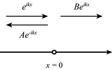
Figure 1: One dimensional space with a point interaction, which is located at $x=0$. The incident wave from the left-hand side is scattered by the point of $x=0$.

The junction condition at the point interaction is provided by the conservation of the probability current

$$j(-0)=j(+0),$$ (3)

where $+0$ and $-0$ denote the limits to zero from above and below, respectively, and the time variable $t$ is abbreviated from now on. Substituting Eq. (2.1) into Eq. (3), we derive

$$\psi^{\ast}(-0)\psi^{\prime}(-0)-\psi(-0){\psi^{\ast}}^{\prime}(-0)$$ (4)

$$=\psi^{\ast}(+0)\psi^{\prime}(+0)-\psi(+0){\psi^{\ast}}^{\prime}(+0),$$

where the prime $(^{\prime})$ denotes the differentiation with respect to $x$. When we introduce new vectors as in [4],

$$\Psi:=\left(\begin{array}[]{c}\psi(+0)\\ \psi(-0)\end{array}\right),\quad\Psi^{\prime}:=\left(\begin{array}[]{c}\psi^{\prime}(+0)\\ -\psi^{\prime}(-0)\end{array}\right),$$ (5)

Eq. (4) can be expressed as

$$\Psi^{\prime\dagger}\Psi=\Psi^{\dagger}\Psi^{\prime},$$ (6)

where $(^{\dagger})$ denotes the transpose of the complex conjugate. Equation (6) is equivalently expressed as

$$\left|\Psi-iL_{0}\Psi^{\prime}\right|=\left|\Psi+iL_{0}\Psi^{\prime}\right|$$ (7)

where $L_{0}\left(\in\mathbb{R}\right)$ is an arbitrary nonvanishing constant with the dimension of length. Thus, $\Psi-iL_{0}\Psi^{\prime}$ is connected to $\Psi+iL_{0}\Psi^{\prime}$ via a unitary transformation. Note that the condition (7) was derived also from the method of a self-adjoint extension of the Hamiltonian in [59], although the notation is slightly different from ours. Therefore, we obtain the junction condition [4]

$$(U-I)\Psi+iL_{0}(U+I)\Psi^{\prime}=0,$$ (8)

where $I$ is the $2\times 2$ identity matrix, and $U$ is a $2\times 2$ unitary matrix, i.e., $U\in U(2)$.

It is sometimes useful to adopt the following parametrization for $U$,

$$U=e^{i\xi I}e^{i\zeta\sigma_{1}}e^{i\eta\sigma_{2}}e^{i\chi\sigma_{3}},$$ (9)

where $\sigma_{i}\ (i=1,2,3)$ denotes the Pauli matrices, and $\xi,\zeta,\eta,\chi\left(\in\mathbb{R}\right)$ are parameters. For example, when we take $\xi=\pi/2$, $\zeta=-\pi/2$, $\eta=\chi=0$, we retrieve a free particle with no interaction, in which $\psi(-0)=\psi(+0)$, $\psi^{\prime}(-0)=\psi^{\prime}(+0)$. When we take $\xi=\left(\theta+\pi\right)/2$, $\zeta=\left(\theta-\pi\right)/2$, $\eta=\chi=0$, where $\theta$ is a parameter, we can derive a potential made of the Dirac delta function $\delta(x)$.

2.2 Parity-invariant junction conditions

We restrict our attention to the parity-invariant junction conditions.

We now introduce the parity transformation ${\cal P}$, which acts on the wave function as

$${\cal P}\psi(x)=\psi(-x).$$ (10)

Since ${\cal P}^{2}\psi(x)=\psi(x)$, the eigenvalues of ${\cal P}$ take $\pm 1$. We assume the eigenstates to be $\psi_{+}$ and $\psi_{-}$ for the eigenvalues $+1$ and $-1$, respectively, i.e.,

$${\cal P}\psi_{\pm}(x)=\pm\psi_{\pm}(x).$$ (11)

The eigenstates $\psi_{\pm}$ are found to be

$$\psi_{\pm}(x)=\frac{\psi(x)\pm\psi(-x)}{2}.$$ (12)

The parity transformations of $\Psi$ and $\Psi^{\prime}$ are given, respectively, by

$$\Psi\stackrel{{\scriptstyle\cal P}}{{\longrightarrow}}\sigma_{1}\Psi,\quad\mbox{and}\quad\Psi^{\prime}\stackrel{{\scriptstyle\cal P}}{{\longrightarrow}}\sigma_{1}\Psi^{\prime}.$$ (13)

We define the projection operators ${\cal P}_{\pm}$ onto the states $\psi_{\pm}$ as

$${\cal P}_{\pm}:=\frac{I\pm\sigma_{1}}{2},$$ (14)

so that we have

$${\cal P}_{+}\Psi=\left(\begin{array}[]{c}\psi_{+}(+0)\\ \psi_{+}(+0)\end{array}\right),\quad{\cal P}_{-}\Psi=\left(\begin{array}[]{c}\psi_{-}(+0)\\ -\psi_{-}(+0)\end{array}\right).$$ (15)

These projection operators satisfy the relations

$$\left({\cal P}_{\pm}\right)^{2}={\cal P}_{\pm},$$ (16)

$${\cal P}_{\pm}{\cal P}_{\mp}=0,$$ (17)

$${\cal P}_{+}+{\cal P}_{-}=I.$$ (18)

The parity transformation of the junction condition (8) becomes

$$(\sigma_{1}U\sigma_{1}-I)\sigma_{1}\Psi+iL_{0}(\sigma_{1}U\sigma_{1}+I)\sigma_{1}\Psi^{\prime}=0,$$ (19)

where $\sigma_{1}$ is multiplied from the left-hand side. Thus the unitary matrix $U$ is transformed under the parity transformation as

$$U\stackrel{{\scriptstyle\cal P}}{{\longrightarrow}}\sigma_{1}U\sigma_{1}.$$ (20)

Therefore, the parity invariance imposes the condition

$$\sigma_{1}U\sigma_{1}=U$$ (21)

on the unitary matrix $U$ for the junction condition.

We can easily show that the unitary matrix $U_{\rm p}$ satisfying the parity-invariant condition (21) is given by $\eta=\chi=0$ for the parametrization of Eq. (9), i.e.,

$$U_{\rm p}=e^{i\xi I}e^{i\zeta\sigma_{1}}.$$ (22)

This class of unitary matrices includes the junction condition for a free particle with no interaction and that for a delta function potential.

Let us derive the parity-invariant junction conditions for the wave function explicitly. For our purpose, we rewrite $U_{\rm p}$ in Eq. (22) as

$$U_{\rm p}=e^{i\theta_{+}}{\cal P}_{+}+e^{i\theta_{-}}{\cal P}_{-},$$ (23)

where we define

$$\theta_{\pm}:=\xi\pm\zeta.$$ (24)

These parameters $\theta_{\pm}$ describe a torus $T^{2}=S^{1}\otimes S^{1}$. Here we have used Eqs. (14), (16)–(18) and the Baker-Campbell-Hausdorff relation [60]

$$e^{X}e^{Y} = \exp\Big{(}X+Y+\frac{1}{2}\left[X,Y\right]$$ (25)

$$+\frac{1}{12}\left(\left[\left[X,Y\right],Y\right]+\left[X,\left[X,Y\right]\right]\right)+\cdots\Big{)},$$

where $\left[X,Y\right]:=XY-YX$. Substituting Eq. (23) into Eq. (8), we derive the junction condition

$$\left(e^{i\theta_{+}}-1\right){\cal P}_{+}\Psi+iL_{0}\left(e^{i\theta_{+}}+1\right){\cal P}_{+}\Psi^{\prime}$$ (26)

$$+\left(e^{i\theta_{-}}-1\right){\cal P}_{-}\Psi+iL_{0}\left(e^{i\theta_{-}}+1\right){\cal P}_{-}\Psi^{\prime}=0.$$

Here we have

$${\cal P}_{+}\Psi^{\prime}=\left(\begin{array}[]{c}\psi^{\prime}_{+}(+0)\\ \psi^{\prime}_{+}(+0)\end{array}\right),\quad{\cal P}_{-}\Psi^{\prime}=\left(\begin{array}[]{c}\psi^{\prime}_{-}(+0)\\ -\psi^{\prime}_{-}(+0)\end{array}\right).$$ (27)

The junction condition (26) can be divided into two parts; one is derived by multiplying Eq. (26) by ${\cal P}_{+}$ from the left-hand side, and the other is derived by multiplying Eq. (26) by ${\cal P}_{-}$ in the same way. The resultant equations are

$$\left(e^{i\theta_{+}}-1\right){\cal P}_{+}\Psi+iL_{0}\left(e^{i\theta_{+}}+1\right){\cal P}_{+}\Psi^{\prime}=0,$$ (28)

$$\left(e^{i\theta_{-}}-1\right){\cal P}_{-}\Psi+iL_{0}\left(e^{i\theta_{-}}+1\right){\cal P}_{-}\Psi^{\prime}=0.$$ (29)

Substituting Eqs. (15) and (27) into Eqs. (28) and (29), we derive

$$\psi_{+}(+0)+L^{(+)}\psi^{\prime}_{+}(+0)=0,$$ (30)

$$\psi_{-}(+0)+L^{(-)}\psi^{\prime}_{-}(+0)=0,$$ (31)

where $L^{(\pm)}\left(\in\mathbb{R}\right)$ are defined as

$$L^{(\pm)}:=L_{0}\cot\frac{\theta_{\pm}}{2}.$$ (32)

When we use Eq. (12), Eqs. (30) and (31) are expressed as

$$\left(\psi(+0)+\psi(-0)\right)+L^{(+)}\left(\psi^{\prime}(+0)-\psi^{\prime}(-0)\right)=0,$$ (33)

$$\left(\psi(+0)-\psi(-0)\right)+L^{(-)}\left(\psi^{\prime}(+0)+\psi^{\prime}(-0)\right)=0.$$ (34)

Consequently, Eqs. (33) and (34) provide the parity-invariant junction conditions for the wave function.

We provide characteristic examples for the parity-invariant junction conditions.

1. Decoupling boundary conditions (Robin boundary conditions).— When $L^{(+)}=L^{(-)}=L$, the junction conditions (33) and (34) reduce to

   $$\psi(+0)+L\psi^{\prime}(+0)=0,$$ (35)

   $$\psi(-0)-L\psi^{\prime}(-0)=0.$$ (36)

   These leads to $j(+0)=j(-0)=0$. Thus, the probability current vanishes at $x=0$. Therefore, the wave function in $x<0$ is completely decoupled from that in $x>0$ in this case.

2. Scale-invariant boundary conditions.— The scale-invariant feature appears in the following cases:

   1. When $\theta_{+}=\theta_{-}=0$, i.e., $L^{(+)}\rightarrow\infty\ (\mbox{or}\ -\infty)$ and $L^{(-)}\rightarrow\infty\ (\mbox{or}\ -\infty)$, we derive

      $$\psi^{\prime}(+0)=\psi^{\prime}(-0)=0.$$ (37)

      This is the Neumann boundary condition.

   2. When $\theta_{+}=\theta_{-}=\pi$, i.e., $L^{(+)}=L^{(-)}=0$, we derive

      $$\psi(+0)=\psi(-0)=0.$$ (38)

      This is the Dirichlet boundary condition.

   3. When $\theta_{+}=0$ and $\theta_{-}=\pi$, i.e., $L^{(+)}\rightarrow\infty\ (\mbox{or}\ -\infty)$ and $L^{(-)}=0$, we derive

      $$\psi(+0)=\psi(-0),\ \mbox{and}\ \psi^{\prime}(+0)=\psi^{\prime}(-0).$$ (39)

      This gives a free particle with no interaction.

   4. When $\theta_{+}=\pi$ and $\theta_{-}=0$, i.e., $L^{(+)}=0$ and $L^{(-)}\rightarrow\infty\ (\mbox{or}\ -\infty)$, we derive

      $$\psi(+0)=-\psi(-0),\ \mbox{and}\ \psi^{\prime}(+0)=-\psi^{\prime}(-0).$$ (40)

      This induces the phase inversion at the boundary.

3. Boundary conditions of the Dirac delta function.— When $\theta_{-}=\pi$, i.e., $L^{(-)}=0$, we derive

   $$\psi(+0)=\psi(-0),$$ (41)

   and

   $$\psi^{\prime}(+0)-\psi^{\prime}(-0)=-\frac{2}{L^{(+)}}\psi(+0).$$ (42)

   This gives a potential by the Dirac delta function.

2.3 Scattering of plane wave

We discuss the scattering of plane wave approaching from the region of $x<0$ by the point interaction as shown in Fig. 1. (See also [62], which is an excellent review.) We assume the wave function as

$$\psi(x)=\left\{\begin{array}[]{ll}e^{ikx}+Ae^{-ikx}&(x<0)\\ Be^{ikx}&(x>0)\end{array}\right.,$$ (43)

where $k(>0)$ denotes the wave number, and $A,B\left(\in\mathbb{C}\right)$ are constants which are determined by the junction conditions. When we adopt the junction conditions (33) and (34) at $x=0$ for the wave function in Eq. (43), we obtain

$$A = -\frac{1+k^{2}L^{(+)}L^{(-)}}{\left(1+ikL^{(+)}\right)\left(1+ikL^{(-)}\right)},$$ (44)

$$B = \frac{ik\left(L^{(+)}-L^{(-)}\right)}{\left(1+ikL^{(+)}\right)\left(1+ikL^{(-)}\right)}.$$ (45)

Note that the same expressions are obtained when the plane wave approaches from the region of $x>0$. This is the natural result from the parity invariance. The transmission probability $T_{1}$ is calculated as

$$T_{1}=\left|B\right|^{2}=\frac{k^{2}\left(L^{(+)}-L^{(-)}\right)^{2}}{\left(1+k^{2}\left(L^{(+)}\right)^{2}\right)\left(1+k^{2}\left(L^{(-)}\right)^{2}\right)}.$$ (46)

It is interesting that $T_{1}$ decreases to zero as $k\rightarrow\infty$ in most cases if $L^{(+)}\neq 0$ and $L^{(-)}\neq 0$. This fact defies our intuition, because even a high energy particle could not penetrate the potential barrier. From the inequality $T_{1}\leq 1$, we also derive

$$\left(L^{(+)}L^{(-)}k^{2}+1\right)^{2}\geq 0.$$ (47)

Therefore, while the transmission probability $T_{1}$ completely vanishes when $L^{(+)}=L^{(-)}$, the perfect transmission (i.e., $T_{1}=1$) occurs when $k=\sqrt{-1/\left(L^{(+)}L^{(-)}\right)}$ if $L^{(+)}L^{(-)}<0$.

3 One-dimensional quantum systems with two parity-invariant point interactions

3.1 Scattering of plane wave by two parity-invariant point interactions

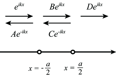
Figure 2: One dimensional space with two point interactions, which are located at $x=-a/2$ and $x=a/2$. The incident wave from the left-hand side is scattered by the points of $x=-a/2$ and $x=a/2$.

Let us discuss quantum mechanics in one spatial dimension with two point interactions, which are located at $x=-a/2$ and $x=a/2$ (see Fig. 2). The wave function is assumed to be

$$\psi(x)=\left\{\begin{array}[]{ll}e^{ikx}+Ae^{-ikx}&\left(x<-\displaystyle\frac{a}{2}\right)\\ Be^{ikx}+Ce^{-ikx}&\left(-\displaystyle\frac{a}{2}<x<\displaystyle\frac{a}{2}\right)\\ De^{ikx}&\left(\displaystyle\frac{a}{2}<x\right)\end{array}\right.,$$ (48)

where $A,B,C,D\left(\in\mathbb{C}\right)$ are constants. In the same way as in Eqs. (33) and (34), the parity-invariant junction conditions at $x=-a/2$ and $x=a/2$ become, respectively,

$$\left\{\psi\left(-\displaystyle\frac{a}{2}+0\right)+\psi\left(-\displaystyle\frac{a}{2}-0\right)\right\}$$ (49)

$$+L^{(+)}_{1}\left\{\psi^{\prime}\left(-\displaystyle\frac{a}{2}+0\right)-\psi^{\prime}\left(-\displaystyle\frac{a}{2}-0\right)\right\}=0,$$

$$\left\{\psi\left(-\displaystyle\frac{a}{2}+0\right)-\psi\left(-\displaystyle\frac{a}{2}-0\right)\right\}$$ (50)

$$+L^{(-)}_{1}\left\{\psi^{\prime}\left(-\displaystyle\frac{a}{2}+0\right)+\psi^{\prime}\left(-\displaystyle\frac{a}{2}-0\right)\right\}=0,$$

and

$$\left\{\psi\left(\displaystyle\frac{a}{2}+0\right)+\psi\left(\displaystyle\frac{a}{2}-0\right)\right\}$$ (51)

$$+L^{(+)}_{2}\left\{\psi^{\prime}\left(\displaystyle\frac{a}{2}+0\right)-\psi^{\prime}\left(\displaystyle\frac{a}{2}-0\right)\right\}=0,$$

$$\left\{\psi\left(\displaystyle\frac{a}{2}+0\right)-\psi\left(\displaystyle\frac{a}{2}-0\right)\right\}$$ (52)

$$+L^{(-)}_{2}\left\{\psi^{\prime}\left(\displaystyle\frac{a}{2}+0\right)+\psi^{\prime}\left(\displaystyle\frac{a}{2}-0\right)\right\}=0.$$

Here, $L^{(+)}_{1}$ and $L^{(-)}_{1}$ characterize the junction conditions at $x=-a/2$, while $L^{(+)}_{2}$ and $L^{(-)}_{2}$ characterize those at $x=a/2$. Solving Eqs. (49)–(52) under the assumption of Eq. (48) with respect to $A,B,C$ and $D$, we derive

$$A = \frac{e^{-ika}}{\Delta}\left\{-\left(1+ikL_{2}^{(+)}\right)\left(1+ikL_{2}^{(-)}\right)\right.$$ (53)

$$\times\left(1+k^{2}L_{1}^{(+)}L_{1}^{(-)}\right)+\left(1-ikL_{1}^{(+)}\right)\left(1-ikL_{1}^{(-)}\right)$$

$$\left.\times\left(1+k^{2}L_{2}^{(+)}L_{2}^{(-)}\right)e^{2ika}\right\},$$

$$B = \frac{ik}{\Delta}\left(L_{1}^{(+)}-L_{1}^{(-)}\right)\left(1+ikL_{2}^{(+)}\right)\left(1+ikL_{2}^{(-)}\right),$$ (54)

$$C = -\frac{ik}{\Delta}\left(L_{1}^{(+)}-L_{1}^{(-)}\right)\left(1+k^{2}L_{2}^{(+)}L_{2}^{(-)}\right)e^{ika},$$ (55)

$$D = -\frac{k^{2}}{\Delta}\left(L_{1}^{(+)}-L_{1}^{(-)}\right)\left(L_{2}^{(+)}-L_{2}^{(-)}\right),$$ (56)

where

$$\Delta = \left(1+ikL_{1}^{(+)}\right)\left(1+ikL_{1}^{(-)}\right)\left(1+ikL_{2}^{(+)}\right)$$ (57)

$$\times\left(1+ikL_{2}^{(-)}\right)-\left(1+k^{2}L_{1}^{(+)}L_{1}^{(-)}\right)$$

$$\times\left(1+k^{2}L_{2}^{(+)}L_{2}^{(-)}\right)e^{2ika}.$$

Then, the transmission probability $T$ is calculated as

$$T_{2}=\left|D\right|^{2}=\frac{k^{4}\left(L_{1}^{(+)}-L_{1}^{(-)}\right)^{2}\left(L_{2}^{(+)}-L_{2}^{(-)}\right)^{2}}{\left|\Delta\right|^{2}}.$$ (58)

If $L_{1}^{(+)}=L_{1}^{(-)}$ or $L_{2}^{(+)}=L_{2}^{(-)}$, then the transmission probability completely vanishes in the same way as the case of a single point interaction.

3.2 Conditions for resonant transmission

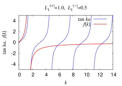
Figure 3: Functions in the resonance condition (77) for $L_{1}^{(+)}+L_{1}^{(-)}>0$ and $L_{1}^{(+)}L_{1}^{(-)}>0$. Here, we adopt $a=1.0$, $L_{1}^{(+)}=1.0$ and $L_{1}^{(-)}=0.5$. The horizontal axis denotes the wave number $k$. Perfect transmission occurs at the points of intersection between the solid (red) curves and the dashed (blue) curves.

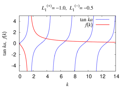
Figure 4: Functions in the resonance condition (77) for $L_{1}^{(+)}+L_{1}^{(-)}<0$ and $L_{1}^{(+)}L_{1}^{(-)}>0$. Here, we adopt $a=1.0$, $L_{1}^{(+)}=-1.0$ and $L_{1}^{(-)}=-0.5$. The horizontal axis denotes the wave number $k$. Perfect transmission occurs at the points of intersection between the solid (red) curves and the dashed (blue) curves.

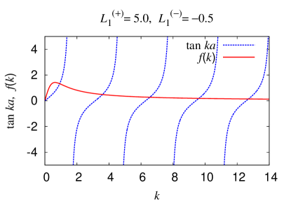
Figure 5: Functions in the resonance condition (77) for $L_{1}^{(+)}+L_{1}^{(-)}>0$ and $L_{1}^{(+)}L_{1}^{(-)}<0$. Here, we adopt $a=1.0$, $L_{1}^{(+)}=5.0$ and $L_{1}^{(-)}=-0.5$. The horizontal axis denotes the wave number $k$. Perfect transmission occurs at the points of intersection between the solid (red) curves and the dashed (blue) curves.

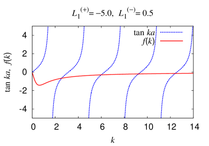
Figure 6: Functions in the resonance condition (77) for $L_{1}^{(+)}+L_{1}^{(-)}<0$ and $L_{1}^{(+)}L_{1}^{(-)}<0$. Here, we adopt $a=1.0$, $L_{1}^{(+)}=-5.0$ and $L_{1}^{(-)}=0.5$. The horizontal axis denotes the wave number $k$. Perfect transmission occurs at the points of intersection between the solid (red) curves and the dashed (blue) curves.

We investigate the conditions for perfect transmission. From the inequality $T_{2}\leq 1$, we obtain

$$\left(M_{11}\sin ka+M_{12}\cos ka\right)^{2}$$ (59)

$$+\left(M_{21}\sin ka+M_{22}\cos ka\right)^{2}\geq 0,$$

where

$$M_{11} = 2\left(1-k^{4}L_{1}^{(+)}L_{1}^{(-)}L_{2}^{(+)}L_{2}^{(-)}\right),$$ (60)

$$M_{12} = -kL_{1}^{(+)}-kL_{1}^{(-)}-kL_{2}^{(+)}-kL_{2}^{(-)}$$ (61)

$$-k^{3}L_{1}^{(+)}L_{1}^{(-)}L_{2}^{(+)}-k^{3}L_{1}^{(+)}L_{1}^{(-)}L_{2}^{(-)}$$

$$-k^{3}L_{1}^{(+)}L_{2}^{(+)}L_{2}^{(-)}-k^{3}L_{1}^{(-)}L_{2}^{(+)}L_{2}^{(-)},$$

$$M_{21} = kL_{1}^{(+)}+kL_{1}^{(-)}-kL_{2}^{(+)}-kL_{2}^{(-)}$$ (62)

$$-k^{3}L_{1}^{(+)}L_{1}^{(-)}L_{2}^{(+)}-k^{3}L_{1}^{(+)}L_{1}^{(-)}L_{2}^{(-)}$$

$$+k^{3}L_{1}^{(+)}L_{2}^{(+)}L_{2}^{(-)}+k^{3}L_{1}^{(-)}L_{2}^{(+)}L_{2}^{(-)},$$

$$M_{22} = -2\left(k^{2}L_{1}^{(+)}L_{1}^{(-)}-k^{2}L_{2}^{(+)}L_{2}^{(-)}\right).$$ (63)

Thus, we derive the following conditions for the perfect transmission, i.e., $T_{2}=1$,

$$M_{11}\sin ka+M_{12}\cos ka = 0,$$ (64)

$$M_{21}\sin ka+M_{22}\cos ka = 0.$$ (65)

These equations with respect to $k$ have solutions if and only if

$$\det\left(\begin{array}[]{cc}M_{11}&M_{12}\\ M_{21}&M_{22}\end{array}\right)=0.$$ (66)

Note that when this equation holds, Eqs. (64) and (65) give one independent equation. The condition (66) is expressed as

$$\alpha k^{4}+2\beta k^{2}+\gamma=0,$$ (67)

where

$$\alpha = \left(L_{1}^{(+)}-L_{1}^{(-)}\right)^{2}\left(L_{2}^{(+)}L_{2}^{(-)}\right)^{2}$$ (68)

$$-\left(L_{2}^{(+)}-L_{2}^{(-)}\right)^{2}\left(L_{1}^{(+)}L_{1}^{(-)}\right)^{2},$$

$$\beta = \left(L_{1}^{(+)}-L_{1}^{(-)}\right)^{2}L_{2}^{(+)}L_{2}^{(-)}-\left(L_{2}^{(+)}-L_{2}^{(-)}\right)^{2}$$ (69)

$$\times L_{1}^{(+)}L_{1}^{(-)},$$

$$\gamma = \left(L_{1}^{(+)}-L_{1}^{(-)}\right)^{2}-\left(L_{2}^{(+)}-L_{2}^{(-)}\right)^{2}.$$ (70)

When all of the coefficients in Eq. (67) vanish, i.e.,

$$\alpha=\beta=\gamma=0,$$ (71)

Eq. (66) is identically satisfied, independent of the value of $k$. Equation (71) gives

$$L_{1}^{(+)}L_{1}^{(-)}=L_{2}^{(+)}L_{2}^{(-)},$$ (72)

$$\left(L_{1}^{(+)}\right)^{2}+\left(L_{1}^{(-)}\right)^{2}=\left(L_{2}^{(+)}\right)^{2}+\left(L_{2}^{(-)}\right)^{2},$$ (73)

which leads to the relations

$$\left(\begin{array}[]{c}L_{2}^{(+)}\\ L_{2}^{(-)}\end{array}\right)=\pm\left(\begin{array}[]{c}L_{1}^{(+)}\\ L_{1}^{(-)}\end{array}\right),\quad\mbox{or}\quad\left(\begin{array}[]{c}L_{2}^{(+)}\\ L_{2}^{(-)}\end{array}\right)=\pm\left(\begin{array}[]{c}L_{1}^{(-)}\\ L_{1}^{(+)}\end{array}\right).$$ (74)

Therefore, when the relations (74) hold, the necessary and sufficient condition (66) is identically satisfied. Then, we can generally obtain solutions for the perfect transmission by solving Eq. (64) or (65).

We investigate all the cases in Eq. (74) in the following.

(i) The cases of $\displaystyle\left(L_{2}^{(+)},L_{2}^{(-)}\right)=\left(L_{1}^{(+)},L_{1}^{(-)}\right)$ or $\left(L_{1}^{(-)},L_{1}^{(+)}\right)$. From Eq. (64) or (65), we derive

$$\left(1+k^{2}L_{1}^{(+)}L_{1}^{(-)}\right)\left\{\left(1-k^{2}L_{1}^{(+)}L_{1}^{(-)}\right)\sin ka\right.$$ (75)

$$\left.-k\left(L_{1}^{(+)}+L_{1}^{(-)}\right)\cos ka\right\}=0.$$

If $L_{1}^{(+)}L_{1}^{(-)}<0$, then we find a solution

$$k=\sqrt{-\frac{1}{L_{1}^{(+)}L_{1}^{(-)}}}.$$ (76)

This result is the same as in the case of a single point interaction. We can also find an infinite number of solutions for perfect transmission through the condition derived from Eq. (75),

$$\tan ka=f(k),$$ (77)

where

$$f(k):=\frac{k\left(L_{1}^{(+)}+L_{1}^{(-)}\right)}{1-k^{2}L_{1}^{(+)}L_{1}^{(-)}}.$$ (78)

The behavior of the function $f(k)$ depends on the signs of $L_{1}^{(+)}+L_{1}^{(-)}$ and $L_{1}^{(+)}L_{1}^{(-)}$. Representative examples in each cases are shown in Figs. 3–6, In these figures, we plot the curves of the functions on the both sides in Eq. (77). At the points of intersection between the solid (red) curves and the dashed (blue) curves, perfect transmission occurs. Consequently, we can find an infinite number of solutions for perfect transmission.

(ii) The cases of $\displaystyle\left(L_{2}^{(+)},L_{2}^{(-)}\right)=\left(-L_{1}^{(+)},-L_{1}^{(-)}\right)$ or $\left(-L_{1}^{(-)},-L_{1}^{(+)}\right)$. From Eq. (64) and (65), we have

$$\left(1-k^{2}L_{1}^{(+)}L_{1}^{(-)}\right)\left(1+k^{2}L_{1}^{(+)}L_{1}^{(-)}\right)\sin ka=0.$$ (79)

$$k\left(L_{1}^{(+)}+L_{1}^{(-)}\right)\left(1+k^{2}L_{1}^{(+)}L_{1}^{(-)}\right)\sin ka=0.$$ (80)

If $L_{1}^{(+)}+L_{1}^{(-)}=0$, we have $L_{1}^{(+)}L_{1}^{(-)}<0$ and $\left(1-k^{2}L_{1}^{(+)}L_{1}^{(-)}\right)>0$. Thus, from Eq. (79), we derive

$$\left(1+k^{2}L_{1}^{(+)}L_{1}^{(-)}\right)\sin ka=0.$$ (81)

If $L_{1}^{(+)}+L_{1}^{(-)}\neq 0$, then we derive Eq. (81) again from Eq. (80). It follows that if $L_{1}^{(+)}L_{1}^{(-)}<0$, we find the solution (76) again. We also find an infinite number of solutions from the condition

$$\sin ka=0.$$ (82)

This leads to the solutions

$$k=\frac{n\pi}{a}\quad\left(n=1,2,3,\cdots\right).$$ (83)

for perfect transmission.

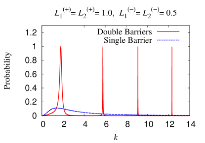
Figure 7: The transmission probability for double barriers is shown as a function of $k$ by the solid (red) curve, when $L_{1}^{(+)}=L_{2}^{(+)}=1.0$ and $L_{1}^{(-)}=L_{2}^{(-)}=0.5$. Here, we adopt $a=1.0$. The perfect transmission ($T_{2}=1$) occurs when the condition $\tan ka=f(k)$ is satisfied. The transmission probability for the single barrier with $L_{1}^{(+)}$ and $L_{1}^{(-)}$ is also shown by the dashed (blue) curve.

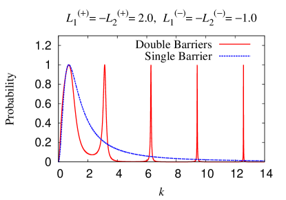
Figure 8: The transmission probability for double barriers is shown as a function of $k$ by the solid (red) curve, when $L_{1}^{(+)}=-L_{2}^{(+)}=2.0$ and $L_{1}^{(-)}=-L_{2}^{(-)}=-1.0$. Here, we adopt $a=1.0$. The first peak appears at $k=\sqrt{-1/(L_{1}^{(+)}L_{1}^{(-)})}$, while the other peaks appear at $k=n\pi/a$. The transmission probability for the single barrier with $L_{1}^{(+)}$ and $L_{1}^{(-)}$ is also shown by the dashed (blue) curve.

We show representative examples of the transmission probability as a function of $k$ for the above cases in Figs. 7 and 8. In these figures, we show the transmission probability for double barriers by the solid (red) curves. We also show the transmission probability for a single barrier by the dashed (blue) curves for comparison. In Fig. 7, we adopt $a=1.0$, $L_{1}^{(+)}=L_{2}^{(+)}=1.0$ and $L_{1}^{(-)}=L_{2}^{(-)}=0.5$, while in Fig. 8, we adopt $a=1.0$, $L_{1}^{(+)}=-L_{2}^{(+)}=2.0$ and $L_{1}^{(-)}=-L_{2}^{(-)}=-1.0$. In these cases, we can confirm the periodic resonant peaks, at which perfect transmission occurs. Furthermore, we find that the peak width decreases as $k$ increases. In particular, when $L_{1}^{(+)}=-L_{2}^{(+)}$ and $L_{1}^{(-)}=-L_{2}^{(-)}$, the transmission probability $T_{2}$ can be expanded around a peak as

$$T_{2}(k)\simeq 1-\left(\frac{k-k_{n}}{w}\right)^{2}+\cdots,$$ (84)

where $k_{n}=n\pi/a$ and

$$w=\frac{k_{n}\left(L_{1}^{(+)}-L_{1}^{(-)}\right)}{2a\left(1+k_{n}^{2}L_{1}^{(+)}L_{1}^{(-)}\right)}\sqrt{T_{1}\left(k_{n},L_{1}^{(+)},L_{1}^{(-)}\right)}$$ (85)

Here, $T_{1}$ is given by Eq. (46). The peak width is roughly given by $w$. Therefore, the peak width is proportional to the square root of the transmission probability for a single barrier and decreases as $k_{n}$ increases. Similar feature could be found also in the case of $L_{1}^{(+)}=L_{2}^{(+)}$ and $L_{1}^{(-)}=L_{2}^{(-)}$.

Let us reconsider the results of Eq. (74) concretely from the view point of potential functions. For example, when we assume a delta function potential at $x=-\frac{a}{2}$, i.e., $V(x)=-\frac{\hbar^{2}}{mL_{1}^{(+)}}\delta(x+\frac{a}{2})$, which is given by $L_{1}^{(+)}\neq 0$ and $L_{1}^{(-)}=0$, an infinite number of resonant peaks appear in the following four cases:

1. $\left(L_{2}^{(+)},L_{2}^{(-)}\right)=\left(L_{1}^{(+)},0\right)$,

2. $\left(L_{2}^{(+)},L_{2}^{(-)}\right)=\left(-L_{1}^{(+)},0\right)$,

3. $\left(L_{2}^{(+)},L_{2}^{(-)}\right)=\left(0,L_{1}^{(+)}\right)$,

4. $\left(L_{2}^{(+)},L_{2}^{(-)}\right)=\left(0,-L_{1}^{(+)}\right)$.

The cases (I) and (II) correspond to the potentials $-\frac{\hbar^{2}}{mL_{1}^{(+)}}\delta(x-\frac{a}{2})$ and $\frac{\hbar^{2}}{mL_{1}^{(+)}}\delta(x-\frac{a}{2})$, respectively. These might be predictable consequences. However, the last two cases (III) and (IV) would be unexpected results.

Finally, it should be noticed that even if Eq. (71) does not hold, the positive solution $k$ satisfying the condition (66) or (67) may exist when the solution of Eq. (67)

$$k^{2}=\frac{-\left(L_{2}^{(+)}-L_{2}^{(-)}\right)\pm\left(L_{1}^{(+)}-L_{1}^{(-)}\right)}{L_{1}^{(+)}L_{1}^{(-)}\left(L_{2}^{(+)}-L_{2}^{(-)}\right)-L_{2}^{(+)}L_{2}^{(-)}\left(L_{1}^{(+)}-L_{1}^{(-)}\right)}$$ (86)

is positive. In this case, Eq. (64) and (65) could be satisfied for a specific value of $a$. Then, the perfect transmission would occur incidentally in this case.

4 Concluding remarks

We have considered the scattering of a quantum particle by two independent, successive parity-invariant point interactions in one dimension. The parameter space is given by the direct product of two tori and described by four parameters $L_{1}^{(+)}$, $L_{1}^{(-)}$, $L_{2}^{(+)}$ and $L_{2}^{(-)}$. By considering incident plane wave, we derived the formula for the transmission probability without any assumptions about the parameter space. Based on the formula, we investigated the conditions for the parameter space under which the perfect resonant transmission occur. Finally, we found the resonance conditions, which are the main results in this paper, to be given by the symmetric and anti-symmetric relations (74) between the parameters

In this paper, we restricted our attention to the parity-invariant point interactions. When we relax this assumption, the parameter space becomes larger, i.e., $U(2)\otimes U(2)$. This extension will be discussed elsewhere [63]. Furthermore, the properties of resonant transmission through $N$ independent multiple point interactions would be future works.

Finally, it should be noted that the analysis of our physical systems from the viewpoint of the $S$ matrix on the complex $k$-plane would also be important future works. From this approach, we could discuss quasi-stationary or resonance states which appear between the two potential barriers, and its lifetime. The authors of [64, 65] investigated the poles of $S$ matrix in the system of a double delta barrier potential. Our physical systems in the present paper give the extension of their system. Therefore, the analysis based on the $S$ matrix would give us a deep understanding of the physical processes.

References

- [1] M. Reed and B. Simon, Methods of Modern Mathematical Physics, Vol. II, Academic Press, New York, 1980.
- [2] P. Šeba, Czeck. J. Phys. 36 (1986) 667.
- [3] S. Albeverio, F. Gesztesy, R. Høegh-Krohn, and H. Holden, Solvable Models in Quantum Mechanics, Springer, New York, 1988.
- [4] T. Cheon, T. Fülöp, and I Tsutsui, Annals of Physics 294, 1 (2001).
- [5] P. Šeba, Reports on Mathematical Physics 24, 111 (1986).
- [6] J. E. Avron, P. Exner, and Y. Last, Phys. Rev. Lett. 72, 896 (1994).
- [7] D. J. Griffiths, J. Phys. A: Math. Gen. 26, 2265 (1993).
- [8] F. A. B. Coutinho, Y Nogami, and J. F. Perezdag, J. Phys. A: Math. Gen. 30, 3937 (1997).
- [9] T. Cheon and T. Shigehara, Physics Letters A 243, 111 (1998).
- [10] F. A. B. Coutinho, Y. Nogami, and J. F. Perez, J. Phys. A: Math. Gen. 32, L133 (1999).
- [11] P. L. Christiansen, H. C. Arnbak, A. V. Zolotaryuk, V. N. Ermakov, and Y. B. Gaididei, J. Phys. A: Math. Gen. 36, 7589 (2003).
- [12] A. V. Zolotaryuk, P. L. Christiansen, and S. V. Iermakova, J. Phys. A: Math. Gen. 39, 9329 (2006).
- [13] F. M. Toyama and Y. Nogami, J. Phys. A: Math. Theor. 40, F685 (2007).
- [14] A. V. Zolotaryuk, J. Phys. A: Math. Theor. 40, 5443 (2007).
- [15] M. Gadella, J. Negro, and L. M. Nieto, Phys. Lett. A 373, 1310 (2009).
- [16] A. V. Zolotaryuk, J. Phys. A: Math. Theor. 43, 105302 (2010).
- [17] A. V. Zolotaryuk, Physics Letters A 374, 1636 (2010).
- [18] A. V. Zolotaryuk and Y. Zolotaryuk, J. Phys. A: Math. Theor. 44, 375305 (2011).
- [19] M. Gadella, M. L. Glasser, and L. M. Nieto, Int. J. Theor. Phys. 50, 2144 (2011).
- [20] A. V. Zolotaryuk, Phys. Rev. A 87, 052121 (2013)
- [21] M. Gadella, M. A. Garcia-Ferrero, and S. Gonzalez-Martin, F. H. Maldonado-Villamizar, Int. J. Theor. Phys. 53, 1614 (2014).
- [22] A. V. Zolotaryuk and Y. Zolotaryuk, Int. J. Mod. Phys. B 28, 1350203 (2014).
- [23] A. V. Zolotaryuk and Y. Zolotaryuk, J. Phys. A: Math. Theor. 48, 035302 (2015).
- [24] A. V. Zolotaryuk, J. Phys. A: Math. Theor. 48, 255304 (2015).
- [25] M. Gadella, J. Mateos-Guilarte, J. M. Munoz-Castaneda, and L. M. Nieto, J. Phys. A: Math. Theor. 49, 015204 (2016).
- [26] R.-J. Lange, J. Math. Phys. 56, 122105-1 (2015).
- [27] T. Cheon, Phys. Lett. A 248, 285 (1998).
- [28] T. Cheon and T. Shigehara, Phys. Rev. Lett. 82, 2536 (1999).
- [29] P. Exner and H. Grosse, arXiv: math-ph/9910029.
- [30] I. Tsutsui, T. Fülöp, and T. Cheon, J. Phys. Soc. Jpn. 69, 3473 (2000).
- [31] T. Fülöp, I. Tsutsui, and T. Cheon, J. Phys. Soc. Jpn. 72, 2737 (2003).
- [32] T. Uchino and I. Tsutsui, Nucl. Phys. B662, 447 (2003); J. Phys. A 36, 6821 (2003).
- [33] T. Nagasawa, M. Sakamoto, and K. Takenaga, Phys. Lett. B562, 358 (2003).
- [34] T. Nagasawa, M. Sakamoto, and K. Takenaga, Phys. Lett. B583, 357 (2004).
- [35] T. Nagasawa, M. Sakamoto, and K. Takenaga, J. Phys. A38, 8053 (2005).
- [36] P. Siegl, J. Phys. A41, 244025 (2008).
- [37] S. Ohya, Ann. Phys. 351, 900 (2014).
- [38] P. Hejačík and T. Cheon, Phys. Lett. A 356, 290 (2006).
- [39] D. Bohm, Quantum Theory, Prentice-Hall, Inc., New York, 1951, p. 283.
- [40] L. V. Iogansen, Soviet Phys. JETP 18, 146, 1964 (J. Exptl. Theoret. Phys. 45, 207, 1963).
- [41] R. Tsu and L. Esaki, Appl. Phys. Lett. 22, 562 (1973).
- [42] L. L. Chang, L. Esaki, and R. Tsu, Appl. Phys. Lett. 24, 593 (1974).
- [43] B. Ricco and M. Y. Azbel, Phys. Rev. B 29, 1970 (1984).
- [44] H. Yamamoto, Applied Physics A Solids and Surfaces 42, 245 (1987).
- [45] A. M. Kriman, N. C. Kluksdahl, D. K. Ferry, and C. Ringhofer, in: D. K. Ferry, C. Jacoboni (Eds.), Quantum Transport in Semiconductors, Plenum Press, New York, 1992, pp. 239-287.
- [46] M. Razavy, Quantum Theory of Tunneling, World Scientific, New Jersey, 2003.
- [47] F. Delgado, J. G. Muga, D. G. Austing, and G. García-Calderón, J. Appl. Phys. 97, 013705 (2005).
- [48] I. Yanetka, Acta Physica Polonica A 116, 1059 (2009).
- [49] I. V. Krive, A. Palevski, R. I. Shekhter, and M. Jonson, Low Temp. Phys. 36, 119 (2010).
- [50] D. J. Vezzetti and M. M. Cahay, Phys. D: Appl. Phys. 19, L53 (1986).
- [51] M. Kalotas and A. R. Lee Eur. J. Phys. 12, 275 (1991).
- [52] D. J. Griffiths and N. F. Taussig, Am. J. Phys. 60, 883 (1992).
- [53] D. W. L. Sprung, H. Wu, and J. Martorell, Am. J. Phys. 61, 1118 (1993).
- [54] M. G. Rozman, P. Reineker, and R. Tehver Phys. Lett. A 187, 127 (1994).
- [55] M. G. Rozman, P. Reineker, and R. Tehver Phys. Rev. A 49, 3310 (1994).
- [56] S. Suzuki, M. Asada, A. Teranishi, H. Sugiyama, and H. Yokoyama, Appl. Phys. Lett. 97, 242102 (2010).
- [57] M. Feiginov, C. Sydlo, O. Cojocari, and P. Meissner, Appl. Phys. Lett. 99, 233506 (2011).
- [58] M. Feiginov, H. Kanaya, S. Suzuki, M. Asada, Appl. Phys. Lett. 104, 243509 (2014).
- [59] G. Bonneau, J. Faraut, and G. Valent, Am. J. Phys. 69, 322 (2001).
- [60] See e.g., W. Greiner and J. Reinhardt, Field Quantization, Springer, Berlin, 1996, p.29.
- [61] P. Kurasov, Journal of Mathematical Analysis and Applications 201, 297 (1996).
- [62] L. J. Boya, Rivista del Nouvo Cimento 31, 75 (2008).
- [63] K. Konno, T. Nagasawa, and R. Takahashi, in preparation.
- [64] E. Hernández, A. Jáuregui, A. Mondragon, et al., Journal of Physics A:Mathematical and General 33, (2000).
- [65] I. E. Antoniou, M. Gadella, E. Hernández, et al., Chaos, Solitons and Fractals 12, 2719 (2001).