Methods for Bayesian Variable Selection with Binary Response Data using the EM Algorithm

Abstract

High-dimensional Bayesian variable selection problems are often solved using computationally expensive Markov Chain Montle Carlo (MCMC) techniques. Recently, a Bayesian variable selection technique was developed for continuous data using the EM algorithm called EMVS. We extend the EMVS method to binary data by proposing both a logistic and probit extension. To preserve the computational speed of EMVS we also implemented the Stochastic Dual Coordinate Descent (SDCA) algorithm. Further, we conduct two extensive simulation studies to show the computational speed of both methods. These simulation studies reveal the power of both methods to quickly identify the correct sparse model. When these EMVS methods are compared to Stochastic Search Variable Selection (SSVS), the EMVS methods surpass SSVS both in terms of computational speed and correctly identifying significant variables. Finally, we illustrate the effectiveness of both methods on two well-known gene expression datasets. Our results mirror the results of previous examinations of these datasets with far less computational cost.
Keywords: High dimension data, EM algorithm, Stochastic Dual Coordinate Ascent, SSVS, EMVS, Variable selection

1 Introduction

The concurrent growth of Bayesian methodology and high dimensional datasets has created a need for high-dimensional Bayesian variable selection techniques. Since George and McCulloch [1993] first introduced Stochastic Search Variable Selection (SSVS), many extensions have been developed for high-dimensional data. Many high-dimensional datasets, especially gene expression data, involve binary responses. Extensions to SSVS have also been developed throughout the literature for high-dimensional data with binary outcomes in Lee et al. [2003], Ai-Jun and Xin-Yuan [2010], and Baragatti [2011]. These Bayesian methods rely on MCMC methods that become computationally costly as the number of covariates grow. Rockova and George [2014] proposed a deterministic alternative using the EM algorithm, which is much faster than most SSVS methods. They present an EM variable selection (EMVS) scheme for continuous data. The main objective of this paper will be to derive EMVS methods for binary response data with both logistic and probit models being considered.

The prior structure for our methods are based on the one used in George and McCulloch [1997] to develop the SSVS method. We use the continuous conjugate versions of the “spike-and-slab” normal mixture formulation which induces a “selective shrinkage” property to aid in variable selection. The probit model is developed with the commonly used data augmentation technique of Albert and Chib [1993]. The recently developed Stochastic Dual Coordinate Ascent (SDCA) method of Shalev-Shwartz and Zhang [2013a] can greatly improve computational times for regularized regression problems such as we have here. A SDCA method is utilized to both speed up the probit model and preserve the computational speed of EMVS for the logistic case. Both of these methods are compared to a probit extensions of the SSVS model that uses a Gibbs sampler along with Metropolis steps from George and McCulloch [1997]. Additionally, the methods developed are available in an R package which can be accessed on the CRAN repository.

The rest of this article is organized as follows: Section 2 characterizes the hierarchical prior for EMVS, as well as the details for implementing the logistic and probit models. Section 3 provides two comprehensive simulation studies that compare both models with each other and to SSVS. In Section 4, we demonstrate both methods on two popular gene expression datasets. Finally, we end with a discussion of our extension of the EMVS technique to binary data in Section 5.

2 Methods for Binary Data

Here we examine both a logistic and probit extension of the original EMVS algorithm for binary data. A key feature of this extension concerns the two methods having nearly the same E-step, but several different derivations in the M-step. For both methods, suppose the response $\bm{y}$ is a vector of length $n$ for $i,\ldots,n$; while $\bm{X}$ represents an $n\times p$ matrix of standardized predictor variables.

2.1 Logistic and Probit likelihoods

For the logistic model, we assume the data have outcomes $y_{i}\in\{\pm 1\}$ and we define $x_{i}\leftarrow-y_{i}x_{i}$. Further, we assume the following data likelihood:

$$f(\bm{y}|\bm{\beta})=\prod_{i=1}^{n}\frac{1}{1+e^{\bm{x}_{i}^{\prime}\bm{\beta}}},$$ (1)

where $\bm{\beta}$ is a vector of length p consisting of the regression coefficients for the model.
A popular alternative to the logistic model for analyzing binary data is the probit model. In the probit model, our data is distributed $y_{i}\sim\text{Bernoulli}(p_{i})$ where $p_{i}=\Phi\left(\bm{x}_{i}^{\prime}\bm{\beta}\right)$ and $\Phi(\cdot)$ is the cumulative distribution function of the standard normal distribution. Note, for the probit model we assume the data have outcomes $y_{i}\in\{0,1\}$. The data likelihood then becomes

$$f(\bm{y}|\bm{\beta})=\prod_{i=1}^{n}\Phi(\bm{x}_{i}^{\prime}\bm{\beta})^{y_{i}}(1-\Phi(\bm{x}_{i}^{\prime}\bm{\beta}))^{1-y_{i}}.$$ (2)

2.2 Spike-and-Slab Prior Structure

As is the case with other Bayesian variable selection techniques, a length p vector $\bm{\gamma}$ of 1’s and 0’s is used for model selection, with the corresponding elements of $\bm{\gamma}$ signifying which columns of $\bm{X}$ are classified as being related to the response. Both models have the following hierarchical prior structure:

$$\pi(\bm{\beta},\sigma,\bm{\gamma})=\pi(\bm{\beta}|\sigma,\bm{\gamma})\pi(\sigma|\bm{\gamma})\pi(\bm{\gamma}).$$ (3)

with the prior on the regression coefficients following a “spike-and-slab” formulation as,

$$\pi(\bm{\beta}|\sigma,\bm{\gamma},\nu_{0},\nu_{1})\propto N_{p}\left(\bm{0},\bm{D_{\sigma,\gamma_{i}}}\right),$$ (4)

where $\bm{D_{\sigma,\gamma_{i}}}=\sigma^{2}\text{diag}(a_{1},\ldots,a_{p})$ and $a_{i}=(1-\gamma_{i})\nu_{0}+\gamma_{i}\nu_{1}$. This means that a variables exclusion or inclusion in the model sets its prior variance as $\nu_{0}$ or $\nu_{1}$ respectively. This formulation was proposed by George and McCulloch [1997], and suggests setting the hyperparameters $\nu_{0}$ and $\nu_{1}$ to be small and large positive values, respectively. Note that we assume that the intercept term has a uniform prior that has been marginalized out of the likelihood function, which is equivalent to centering the data at 0. The prior for $\sigma^{2}$ is conveniently set to be a noninformative Inverse Gamma prior, which is conjugate for the normal family:

$$\pi(\sigma^{2}|\bm{\gamma},\lambda,\nu)\propto IG\left(\frac{\nu}{2},\frac{\nu\lambda}{2}\right),$$ (5)

where $\nu=1$ and $\lambda=1$ to make the prior relatively noninformative. Note that George and McCulloch [1997] suggests that setting these hyperparameters as such suggest that $\lambda$ is the prior estimate of variance $\sigma^{2}$ and $\nu$ can be viewed as a prior sample size used to get that estimate. In formulating a prior for $\bm{\gamma}$, we will use the common Bernoulli-beta setup as:

$$\begin{split}\pi(\bm{\gamma}|\theta)\propto\ &\>\theta^{\sum_{i}{\gamma_{i}}}\left(1-\theta\right)^{p-\sum_{i}{\gamma_{i}}},\\ \pi(\theta)\propto\ &\>\theta^{a-1}(1-\theta)^{b-1},\end{split}$$ (6)

where $\theta$ can be viewed as the probability that any particular variable is in the model.

2.3 EM Algorithm

In order to estimate the unknown parameters $\bm{\beta},\theta,\sigma,$ and $\bm{\gamma}$, the EM algorithm is used instead of the more popular MCMC method, because the algorithm offers substantial computational advantages when p is large. In this implementation of the EM algorithm, the variable inclusion vector $\bm{\gamma}$ is used as the latent variable. Since this variable cannot be observed, it will be replaced by its conditional expected value for the M-step, which will maximize the complete posterior with respect to $\Theta=(\bm{\beta},\theta,\sigma)$. Recall that the EM algorithm maximizes the complete data log likelihood function with the latent variable replaced by its conditional expected value and the other parameters being replaced by their values from the previous iteration. In other words, we will iteratively maximize the objective function

$$\begin{split}Q\left(\bm{\beta},\theta,\sigma|\bm{\beta}^{(k)},\theta^{(k)},\sigma^{(k)},\bm{y}\right)=E_{\bm{\gamma}|.}\left[\log{\pi\left(\bm{\beta},\theta,\sigma,\bm{\gamma}|\bm{y}\right)}|\bm{\beta}^{(k)},\theta^{(k)},\sigma^{(k)},\bm{y}\right].\end{split}$$ (7)

The derivation of $\log{(\pi\left(\bm{\beta},\theta,\sigma,\bm{\gamma}|\bm{y}\right)})$ is different for the logistic and probit model. The objective function $Q$ can be partitioned into two parts, $Q_{1}$ and $Q_{2}$ due to the conjugate nature of the hierarchical prior structure, so that:

$$\begin{split}Q\left(\bm{\beta},\theta,\sigma|\bm{\beta}^{(k)},\theta^{(k)},\sigma^{(k)},\bm{y}\right)=C+Q_{1}\left(\bm{\beta},\sigma|\bm{\beta}^{(k)},\theta^{(k)},\sigma^{(k)}\right)+Q_{2}\left(\theta|\bm{\beta}^{(k)},\theta^{(k)},\sigma^{(k)}\right)\end{split}$$ (8)

where C represents terms which are constant with respect to $\Theta$. Since the logistic and probit models have different likelihoods, the form of $Q_{1}\left(\bm{\beta},\sigma|\bm{\beta}^{(k)},\theta^{(k)},\sigma^{(k)}\right)$ is unique to each of the two models. One can show that for both models

$$Q_{2}\left(\theta|\bm{\beta}^{(k)},\theta^{(k)},\sigma^{(k)}\right)=\sum\limits_{i=1}^{p}{\log{\left(\frac{\theta}{1-\theta}\right)}}E_{\bm{\gamma}|.}\gamma_{i}+(a-1)\log{\theta}+(p+b-1)\log{(1-\theta)}.$$ (9)

This separability of $Q$ allows one to maximize the functions separately in the M-step.

2.4 E-Step

To compute the E-step, we must take the expectation of the aforementioned $Q$ function with respect to the latent variable $\bm{\gamma}$. There are two parts of the formulations that need further examination, namely, $E_{\bm{\gamma}|.}\left[\frac{1}{\nu_{0}(1-\gamma_{i})+\nu_{1}\gamma_{i}}\right]$ and $E_{\bm{\gamma}|.}(\gamma_{i})$. First, as Rockova and George [2014] discuss, the expectation of the latent variable depends on $\bm{y}$ only through $\left(\bm{\beta}^{(k)},\theta^{(k)},\sigma^{(k)}\right)$ because of the hierarchical structure of $\bm{\gamma}$, therefore we have

$$\begin{split}E_{\bm{\gamma|.}}(\gamma_{i})=P\left(\gamma_{i}=1|\bm{\beta}^{(k)},\theta^{(k)},\sigma^{(k)}\right)=p_{i}^{*}.\end{split}$$ (10)

By an application of Bayes formula, we have

$$\begin{split}p_{i}^{*}=\frac{\pi(\beta_{i}^{(k)}|\sigma^{(k)},\gamma_{i}=1)P(\gamma_{i}=1|\theta^{(k)})}{\pi(\beta_{i}^{(k)}|\sigma^{(k)},\gamma_{i}=1)P(\gamma_{i}=1|\theta^{(k)})+\pi(\beta_{i}^{(k)}|\sigma^{(k)},\gamma_{i}=0)P(\gamma_{i}=0|\theta^{(k)})}.\end{split}$$ (11)

Second, from the posterior distribution $\pi(\bm{\gamma}|.)$, we find the other conditional expectation by taking a weighted sum of the precision parameters

$$\begin{split}E_{\bm{\gamma}|.}\left[\frac{1}{\nu_{0}(1-\gamma_{i})+\nu_{1}\gamma_{i}}\right]=\frac{E_{\bm{\gamma}|.}(1-\gamma_{i})}{\nu_{0}}+\frac{E_{\bm{\gamma|.}}\gamma_{i}}{\nu_{1}}=\frac{1-p_{i}^{*}}{\nu_{0}}+\frac{p_{i}^{*}}{\nu_{1}}\equiv d_{i}^{*}.\end{split}$$ (12)

2.5 Logistic Model

If we use the Gaussian mixture prior on $\bm{\beta}$ and the hierarchical prior structure described above; EMVS for logistic regression begins with the E-step in Section 2.4. Next we derive the M-step for logistic regression with EMVS. Substituting in the log of (1), $Q_{1}$ yields the form

$$Q_{1}=-\sum\limits_{i=1}^{n}\text{log}(1+e^{-x_{i}^{\prime}\bm{\beta}})-\frac{p+\nu+2}{2}\log{\sigma^{2}}-\frac{\nu\lambda}{2\sigma^{2}}- \frac{\sum{\beta_{i}^{2}}}{2\sigma^{2}}E_{\bm{\gamma}|.}\left[\frac{1}{\nu_{0}(1-\gamma_{i})+\nu_{1}\gamma_{i}}\right].$$ (13)

Differentiating $Q_{1}$ with respect to $\bm{\beta}$ reveals the following form for $\bm{\beta}^{(k+1)}$:

$$\bm{\beta}^{(k+1)}=\text{arg}\min_{\bm{\beta}}\sum\limits_{i=1}^{n}\text{log}(1+e^{-x_{i}^{\prime}\bm{\beta}})+\|\bm{D}^{\bm{*}1/2}\bm{\beta}\|^{2},$$ (14)

where $\bm{D^{*}}$ is a $p\times p$ diagonal matrix such that $\bm{D^{*}}=\text{diag}\{d_{1}^{*},\cdots,d_{p}^{*}\}$. This is a difficult minimization problem due to the non-linearity associated with the first term in (14).

The regularized logistic model could be solved iteratively using the common Newton-Raphson numerical technique; however, in high dimensions the Newton-Raphson technique is known to be computationally expensive. Instead, we use the suggestion of Rockova and George [2014] and use a Stochastic Dual Coordinate Ascent (SDCA) algorithm from Shalev-Shwartz and Zhang [2013a] to solve (14).

From (13), one can show that for logistic regression

$$\sigma^{(k+1)}=\sqrt{\frac{\|\bm{D}{\bm{*}1/2}\bm{\beta}^{(k+1)}\|^{2}+\nu\lambda}{p+\nu+2}}.$$ (15)

To finish the specification of the M-step, one can show that from (9) that $\theta^{(k+1)}$ has the form

$$\theta^{(k+1)}=\frac{\sum\limits_{i=1}^{n}{p_{i}^{*}}+a-1}{a+b+p-2}.$$ (16)

2.5.1 Stochastic Dual Coordinate Ascent Algorithm

The advantage of the using a SDCA method to solve (14) over the Newton-Raphson technique lies in the computational speed of SDCA. We start by describing the general SDCA algorithm presented in Shalev-Shwartz and Zhang [2013a]. Suppose we want to solve the following general regularization problem

$$\min_{\bm{w}\in\mathbb{R}^{n}}\ P(\bm{w})=\left[\frac{1}{n}\sum\limits_{i=1}^{n}\phi_{i}(\bm{x}_{i}^{\prime}\bm{w})+\frac{\lambda}{2}\|\bm{w}\|^{2}\right],$$ (17)

where $\phi_{i}$ is a scalar convex function. One should note that $\lambda$ is a scalar in (17), whereas for our EMVS model, $\lambda$ is presented as a vector. The goal is to find a $\bm{w^{*}}$ that minimizes (17). For regularized logistic regression we have, $\phi_{i}(a)=\text{log}(1+\text{exp}(-y_{i}a))$. A common technique for solving regularized optimization problems involves finding the dual of the original function. If we let $\phi_{i}^{*}$ denote the convex conjugate of $\phi_{i}$, one can show the dual for $P(\bm{w})$ is:

$$\max_{\bm{\alpha}\in\mathbb{R}^{n}}\ \text{D}(\bm{\alpha})=\left[\frac{1}{n}\sum\limits_{i=1}^{n}-\phi_{i}^{*}(-\alpha_{i})+\left\|\frac{1}{\lambda n}\sum\limits_{i=1}^{n}\bm{x}_{i}^{\prime}\bm{\alpha}_{i}\right\|^{2}\right].$$ (18)

In the case of regularized logistic regression $-\phi_{i}^{*}(-b)=-by_{i}\text{log}(by_{i})+(1-by_{i})\text{log}(1-by_{i})$. Note that $\alpha_{i}$ is the dual for the $i$^th observation. This type of optimization method is often referred to as Dual Coordinate Ascent (DCA). DCA requires only one single $\alpha_{i}$ to be optimized at each iteration. The Shalev-Shwartz and Zhang [2013b] method is stochastic because one randomly picks which $\alpha_{i}$ to optimized at each iteration. Finally, to complete the problem, define $w(\bm{\alpha})=\frac{1}{\lambda n}\sum\limits_{i=1}^{n}\bm{x}_{i}^{\prime}\bm{\alpha}_{i}$ and use the fact that $w(\bm{\alpha^{*}})=w^{*}$ and $\text{P}(\bm{w^{*}})=\text{D}(\bm{\alpha^{*}})$ where $\bm{w^{*}}$ and $\bm{\alpha^{*}}$ are the solution to (17) and (18), respectively. The goal of SDCA is to find values of $\bm{\alpha}$ and $\bm{w}$ to minimize the so-called duality gap defined as $\text{P}(w(\bm{\alpha}))-\text{D}(\bm{\alpha})$. In order to use SDCA for logistic regression as described in Shalev-Shwartz and Zhang [2013a], one still needs to use a few Newton-Raphson steps at each M-step. Shalev-Shwartz and Zhang [2013b] introduced a sightly more efficient SDCA algorithm called Proximal Stochastic Dual Coordinate Ascent (Prox-SDCA) that avoids any Newton-Raphson steps. In the appendix, we present the Prox-SDCA algorithm used to solve (14).

2.6 Probit Model

The likelihood for the probit model (2), is largely intractable, and becomes very complicated when we find the joint posterior distribution. For computational ease, we use the data augmentation method similar to the one proposed by Albert and Chib [1993] to introduce a latent variable $Z_{i}\sim N(\textbf{x}_{i}^{\prime}\bm{\beta},1)$ such that

$$Y_{i}=\left\{\begin{array}[]{l l}1,&\quad\text{if $Z_{i}>0$},\\ 0,&\quad\text{if $Z_{i}\leq 0$}.\end{array}\right.$$

If we observe $\bm{y}$ but $\bm{Z}$ is unobserved, then the distribution of $Z_{i}$ conditioned on $\bm{y}$ is truncated normal, with mean $\bm{x}_{i}^{\prime}\bm{\beta}$ and unit variance. If $y_{i}=1$, then the distribution of $Z_{i}$ is truncated on the left by 0 (denoted by $p_{1}(\cdot)$), otherwise $y_{i}=0$ and the distribution of $Z_{i}$ is truncated on the right by 0 (denoted by $p_{2}(\cdot)$). Note that if we observe $Z_{i}$, then $Z_{i}\sim N(\bm{x}_{i}^{\prime}\bm{\beta},1)$. The idea is to impute $\bm{z}$ so that we can then deal with normally distributed, continuous data rather than binary data. This technique vastly improves computational complexity and efficiency.

Because we do not “observe” our data, we need to add a step to impute it during the E-step of each iteration of the EM algorithm. We estimate $\textbf{z}^{(k)}|\bm{x},\bm{y},\bm{\beta}$, by finding

$$z_{i}^{(k)}=E[z_{i}|\bm{x},\textbf{y},\bm{\beta}^{(k)}]=\left\{\begin{array}[]{l l}\bm{x}_{i}^{\prime}\bm{\beta}^{(k)}+\frac{-\phi(-\bm{x}_{i}^{\prime}\bm{\beta}^{(k)})}{\bm{\Phi}(-\bm{x}_{i}^{\prime}\bm{\beta}^{(k)})},&\quad\text{if $y_{i}=0$}\\ \bm{x}_{i}^{\prime}\bm{\beta}^{(k)}+\frac{\phi(-\bm{x}_{i}^{\prime}\bm{\beta}^{(k)})}{1-\bm{\Phi}(-\bm{x}_{i}^{\prime}\bm{\beta}^{(k)})},&\quad\text{if $y_{i}=1$}.\end{array}\right.$$

This follows from the properties of the truncated normal distribution. Now that we have estimates for $\bm{z}^{(k)}|\bm{x},\bm{y},\bm{\beta}$, we can treat them as the data during each iteration of the EM algorithm so that the objective function becomes

$$\begin{split}Q\left(\bm{\beta},\theta,|\bm{\beta}^{(k)},\theta^{(k)},\bm{z}^{(k)}\right)=E_{\bm{\gamma}|.}\left[\log{\pi\left(\bm{\beta},\theta,\bm{\gamma}|\bm{z}^{(k)}\right)}|\bm{\beta}^{(k)},\theta^{(k)},\bm{z}^{(k)}\right].\end{split}$$ (19)

With the above objective function in hand, one can derive the probit E-M algorithm with relative ease. There are two different methods for estimating $\bm{\beta}^{(k+1)}$ in the M-step. The more traditional generalized ridge regression solution could be used, as well as a more computationally efficient solution such as the SDCA algorithm for continuous data from Shalev-Shwartz and Zhang [2013a]. Our specific E and M steps for the probit model are detailed in the appendix.

3 Simulation

3.1 Method for Simulation of Data

To generate a design matrix, we use the method of Gui and Li [2005]. This method allows us to consider a synthetic data set where $p\gg n$, but a very small number of variables, $p_{\gamma}$, are actually related to the survival time. The remaining $p-p_{\gamma}$ variables are not related to the survival time, but can be correlated with the related ones.

The process, as described in Gui and Li [2005], starts by generating an $n\times p$ matrix $A$ of $U(-1.5,1.5)$ random variables. We then take the first $p_{\gamma}$ columns in this matrix as the related variables that will be used to generate response data. To generate the unrelated variables, we start by obtaining a normalized basis of $A$ using Gram-Schmidt orthonormalization, which we denote as $\left\{\upsilon_{1},\ldots,\upsilon_{p_{\gamma}},\varrho_{1},\ldots,\varrho_{n-p_{\gamma}}\right\}$.

An application of Cauchy’s inequality can be used to show that for any $p_{\gamma}\times(n-p_{\gamma})$ matrix $\bm{T}$,

$$\rho=corr\left(\bm{\upsilon}y,\left(\bm{\varrho}+\bm{\upsilon}\bm{T}\right)x\right)\leq\frac{\lambda}{\sqrt{1+\lambda^{2}}},\,\forall y\in\mathbb{R}^{p_{\gamma}},\forall x\in\mathbb{R}^{n-p_{\gamma}},$$ (20)

where $\lambda^{2}$ is the largest eigenvalue of $\bm{T}^{\prime}\bm{T}$.
We then find $\lambda^{2}=\frac{\rho^{2}}{1-\rho^{2}}$ , where $\rho$ is the desired maximum correlation between the related and unrelated variables. Finally, $\bm{T}$ is then constructed as a diagonal matrix with its largest value as $\lambda$, and the remaining $p-p_{\gamma}$ variables are generated from the linear space $C=\left\{\bm{\varrho}+\bm{\upsilon}T\right\}$.

3.2 Simulation for binary data

Using the method described in Section 3.1, a design matrix $\bm{X}$ is generated with 0.6 chosen as the maximum correlation between related and unrelated variables. Suppose we set $\bm{\beta}=(1,2,3,0,0,\ldots,0)^{\prime}$ so only the first 3 variables are significant and $\epsilon\sim\text{N}_{n}(\bm{0},\sigma^{2}_{\epsilon}\text{I}_{n})$ with $\sigma^{2}_{\epsilon}=3$. Then, we can generate continuous responses through $\bm{y}=\bm{X}\bm{\beta}+\epsilon$. We transform the aforementioned continuous vector $\bm{y}$ for the logistic and probit models. The continuous outcomes are transformed using the transformation $p_{i}=1/(1+\text{exp}(-y_{i}))$. The binary outcome is defined such that, P$(y_{i}=1)=p_{i}$ for both logistic and probit, while for logistic, P$(y_{i}=-1)=1-p_{i}$, and for probit, P$(y_{i}=0)=1-p_{i}$. For both methods we varied $\nu_{0}$, while fixing $\nu_{1}=1000$ in the logistic case and $\nu_{1}=100$ in the probit case. Further, we used the prior $\theta\sim\text{U}(0,1)$, which leads to a beta-binomial prior for $\bm{\gamma}$. Similar to Rockova and George [2014], we set the starting values $\sigma^{(0)}=1$ and $\theta^{(0)}=.5$ . The hyper-parameter $\lambda$ is set to .001 for the logistic model while $\nu$ is set to 1. Since the model is extremely sparse, we use the suggestion from Rockova and George [2014] of setting $a=1$ and $b=p$ . For sparse settings such as this, $b=p$ appears to produce more accurate results.

We are able to set the number of iterations to $K=5,000$ due to the speed of the SDCA and Prox-SDCA algorithms. Setting $K$ any higher results in very slight gains in accuracy. In practice, values of $K$ will be application dependent. Overall, EMVS for logistic regression has fast computational times due to the use of Prox-SDCA. The whole algorithm typically converged in under 10 seconds on a quad core 3.4GHz i7 with 8GB of RAM running Windows 7. We found estimating $\bm{\beta}$ with the SDCA algorithm resulted in similar run times for the probit model. As shown in Figure 1 and Figure 2, we ran both models over a grid of 50 different $\nu_{0}$ values. The values of $\nu_{0}$ ran from 1.02 to 2 by increments of .02 for the logistic model; while for the probit model, values of $\nu_{0}$ stretched from .0002 to .01 with increments of .0002. Recall that $\gamma_{i}$ is the posterior probability of the $i^{\text{th}}$ variable being included in the model. Note that in Figure 1 and Figure 2, variables that have a $\gamma_{i}$ less than .5 are shown between the two red lines. We found that in general, the logistic model preformed better for larger values of $\nu_{0}$ while the probit model preformed better for smaller values. Figure 2 portrays the $\bm{\beta}$ estimates for the probit model with both the GRR estimator and the SDCA algorithm. With $p=1000$ and the number of iterations for the SDCA algorithm equal to 6000, the GRR estimator and the SDCA algorithm produce similar results with comparable run times. As one increases $p$, the SDCA algorithm becomes increasingly computationally efficient compared to the GRR estimator. One option for getting starting values for the EMVS algorithm involves using a regularized logistic estimator. In particular, we could use the Prox-SDCA Algorithm above to get robust starting values for logistic regression. This strategy was employed to produce Figure 1 and Figure 2.

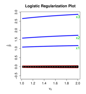
Figure 1: Using EMVS for logistic Regression method, values of estimated regression parameters are plotted across different values of $\nu_{0}$. Only the first three parameters that were set as significant in the true model are found to be significant by the EMVS model.

(a)

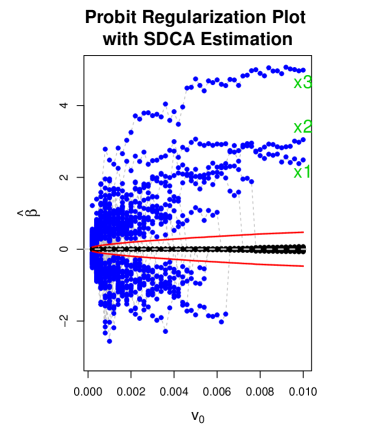
(b)

Figure 2: (a) Uses GRR estimation to estimate regression parameters for the probit model. Estimates are relatively stable across different values of $\nu_{0}$. (b) uses a SDCA algorithm to estimate parameters for the probit model, leading to more volatile estimates across different values of $\nu_{0}$.

3.3 Comparison with Stochastic Search Variable Selection

To demonstrate the power of our EMVS methods, we compared our results to a SSVS model calibrated for binary data. For the sake of comparison, we used the same conjugate spike-and-slab prior for the SSVS model. We closely followed the Metropolis algorithm from George and McCulloch [1997] that also used a conjugate prior structure. Conveniently, under the conjugate spike-and-slab prior the marginal posterior for $\bm{\gamma}$ does not depend on $\bm{\beta}$, hence for the continuous case one only needs to sample $\bm{\gamma}$. For binary data we once again use the data augmentation technique of Albert and Chib [1993] to work with continuous latent variables. In order to sample the latent variables, we must also sample $\bm{\beta}$. Thus, the SSVS algorithm becomes a Gibbs sampler with Metropolis steps to find $\bm{\gamma}$. Further, the data is simulated exactly the same as described in Section 3.2. The same beta-binomial prior is used as above with $\theta\sim U(0,1)$, along with setting $\nu_{0}=0$ and $\nu_{1}=1000$. We set the number of iterations equal to the time it took the EMVS model for logistic regression to go through 50 values of $\nu_{0}$. The SSVS model only got through 700 iterations of the entire Gibbs sampler and performed 700,000 iterations of the Metropolis algorithm in the time it took the EMVS method to complete. The SSVS had an acceptance rate of .006. Recall, we generated the data with $\bm{\beta}=(1,2,3,0,0,\ldots,0)^{\prime}$. The SSVS technique selected a model that only included the predictor $\{\beta_{3}\}$ opposed to both the logistic and probit with EMVS which selected a model that included all 3 significant predictors, $\{\beta_{1},\beta_{2},\beta_{3}\}$. Thus, the developed EMVS techniques for binary data were both faster and better at correctly identifying the significant variables than the SSVS methods.

3.4 Simulation Study

While the simulation studies in Section 3.2 and 3.3 illustrate the power of our EMVS methods for binary data, the selected “true”$\bm{\beta}$ values were rather arbitrary. To further study our developed methods, we created a second simulation which produced a variety of realistic datasets with less arbitrary true $\bm{\beta}$ values. We used the following algorithm for the second simulation:

1. Fix $n=100,p=1000,p_{\gamma}=10,\rho=.6,\sigma^{2}_{\epsilon}=3,$ and $\beta_{max}$.

2. Generate an $n\times p$ design matrix $\mathbf{X}$ using the method outlined in 3.1, such that $p_{\gamma}$ variables will be related to the response and have maximum correlation $\rho$ with the remaining $p-p_{\gamma}$ variables.

3. Generate $p_{\gamma}$ true coefficients from $UNIF(-\beta_{max},\beta_{max})$, and set the remaining $p-p_{\gamma}$ coefficients to 0.

4. Generate continuous response data and convert this to binomial data.

5. Evaluate the probit and the logit methods with respect to True Positive Rate, True Negative Rate, Positive Predictive Value, and Negative Predictive value.

6. Repeat steps 2-5 500 times.

This method was done for $\beta_{max}$ values of 0.5, 1, 2, and 3. The results indicated that the logistic method excels in with larger values of $\nu_{0}$, while probit excels with smaller values, confirming our earlier observation and mirroring performance in real applications. The plot for $\beta_{max}=2$ is shown below. The plots for the other values of $\beta_{max}$ are in the Appendix and show similar patterns, only shifting vertically depending on the magnitude of $\beta_{max}$.

Figure 3: TPR, TNR, PPV, and NPV for the logit and probit models over the tuning parameter $\nu_{0}$ for 500 simulated datasets using a maximum effect size of 2.

Other than as a demonstration of where each data model performs best with respect to the tuning parameter $\nu_{0}$, these plots indicate that the probit model, with its lower true positive rate and almost perfect positive predictive value, is a more conservative model for binary data. The logit model, on the other hand, has a higher true positive rate but a lower positive predictive value, meaning we can be less certain a variable is actually related to the response should it be selected by the method.

4 Applications

4.1 Logistic Application to Leukemia Data

The well studied leukemia dataset from Golub et al. [1999] provides a good benchmark to evaluate the EMVS algorithm with logistic regression. We also analyzed the results from Lee et al. [2003], which used the same leukemia dataset as Golub et al. [1999] with a Bayesian stochastic search algorithm. Lee et al. [2003] provides an ideal comparison since the usefulness of the EMVS algorithm lies in its computational speed compared to other Bayesian variable selection techniques. For comparison purposes, we used the same 38 sample training data set that Lee et al. [2003] and Golub et al. [1999] analyzed. Further, the design matrix was centered and scaled. The leukemia dataset contains 7,129 genes with the binary responses acute myeloid leukemia (AML) or acute lymphoblastic leukemia (ALL). We used the same hyper-parameters as described in Section 3.2, as well as the Prox-SDCA algorithm to get starting values. For the Prox-SDCA algorithm, setting the number of iterations equal to 10 times the number of samples, T=380, produced optimal results. With such a low number of iterations, the whole algorithm takes only 30 seconds to complete. Overall, this is a huge improvement in computational time compared to previous methods. Specifically, Ai-Jun and Xin-Yuan [2010] reported that their SSVS analysis of this dataset took 282 minutes. Genes that had posterior probabilities greater that .5 were considered significant. In Table 1, 18 of 32 genes that were identified as significant were also identified by either Golub et al. [1999] or Lee et al. [2003].

Frequency ID	Gene ID	Frequency ID	Gene ID
461	D49950	1249	L08246**
1745	M16038	1779	M19507
1829	M22960	1834	M23197
1882	M27891	2020	M55150**
2111	M62762**	2121	M63138**
2181	M68891	2242	M80254**
2267	M81933	2288	M84526
2402	M96326*	3258	U46751**
3320	U50136**	3525	U63289
3847	U82759**	4052	X04085**
4196	X17042**	4229	X52056
4377	X62654	4499	X70297
4847	X95735*	5039	Y12670**
5954	Y00339	6041	L09209*
6376	M83652**	6539	X85116
6677	X58431	6919	X16546

Table 1: EMVS with logistic regression for $\nu_{0}=7$. The stared(*) genes were also identified as significant in Lee et al. [2003], while the double stared(**) genes were identified as significant in Golub et al. [1999]. The bolded genes were recognized as significant in both papers.

To analyze the predictive power of the model, we randomly divided the full original leukemia data into a test and training dataset. The original dataset, before it was split, had 72 samples. Further, 48 observations were randomly selected for the training dataset while the remaining observations were left for the test dataset. The data was pre-processed as described in Dudoit et al. [2000]. After pre-processing, the dataset now contained 3,571 genes. All 3,571 genes were used to produce predictions. Using a cut-off of .5, the model correctly predicted 23 out of the 24 observations from the test data set. Lee et al. [2003] found similar results with their stochastic variable selection model, although they only used the significant variables to produce predictions.

4.2 Probit Application to Colon Cancer Data

Another well-studied data set is the colon cancer gene expression data set collected by Alon et al. [1999]. In the study, 40 tumor and 22 normal colon tissues were analyzed with Affymetrix oligonucleotide array to extract useful gene expression patterns from over 6,500 genes. Alon et al. [1999] then selected a subset of 2,000 genes based on the confidence in expression levels. This data has been analyzed extensively in the literature using many different statistical methods, including clustering [Alon et al., 1999, Ben-Dor et al., 2000, Li et al., 2001], support vector machines [Ben-Dor et al., 2000, Furey et al., 2000], boosting [Ben-Dor et al., 2000], partial least squares [Nguyen and Rocke, 2002], and evolutionary neural networks [Kim and Cho, 2004]. Nearly all of these studies used some sort of method of feature selection to reduce noise and improve prediction, so comparison between methods is somewhat limited. Usefulness of gene selection prior to analysis is heavily dependent on the method used for prediction. Additionally, five tissues that were suspected to be contaminated (N34, N36, T30, T33, and T36)[Alon et al., 1999, Li et al., 2001] were removed from analysis.

The gene expression levels were log-transformed prior to analysis, and a repeated random sub-sampling validation scheme was used. Thirty random samples were constructed, in which 20% of the observations were held out, and then the model was fit using the remaining 80% of each sample. Prediction accuracy was averaged over these 30 subsamples, and the best identified genes were those identified most frequently from the 30 models. A gene was considered “significant” if the posterior probability was greater than 0.5, although posterior probabilities tended to be very close to 0 or very close to 1. Table 2 below shows the most commonly identified genes.

Frequency ID	Gene ID	Frequency ID	Gene ID
245	M76378*	897	H43887*
249	M63391*	1042	R36977*
267	M76378*	1058	M80815*
365	X14958*	1325	T47377*
377	Z50753*	1423	J02854
493	R87126*	1582	X63629*
561	R46753	1635	M36634*
625	X12671*	1771	J05032*
698	T51261	1772	H08393*
780	H40095*	1836	U14631
802	X70326*	1870	H55916*
822	T92451*	1884	R44301
892	U31525	1894	X07767

Table 2: Genes with (*) were identified by other methods.

Figure 4: This plot shows the frequency with which genes were selected when fitting the model to 30 subsamples of the data.

Many of the commonly identified genes have also been identified in other studies such as Ben-Dor et al. [2000], Kim and Cho [2004]. Table 2 lists the top 26 genes, but most of the 111 genes identified by EMVS had been identified by other papers as well. A nice feature of data analysis using EMVS is that there is a clear distinction between variables which should be kept in the model as posterior probabilities are either very close to 1 or 0. Most other feature selection methods for this data set have used various scoring procedures with a subjective cutoff used to select the “top” genes. With EMVS, there is no ambiguity as to which variables should be used.

Additionally, for each of the 30 random subsamples used for cross-validation, prediction was very accurate. The average prediction success rate was 93%; the range of success rates using other methods ranges from 72% to 94% [Kim and Cho, 2004]. 17 of the 30 subsamples had 100% prediction success rate. At the very worst, 3 of 11 observations were misclassified.

5 Discussion

In this paper, we developed two methods for Bayesian variable selection when the data has a binary outcome. The main advantage of our method compared to previous Bayesian variable selection for high-dimensional data is a vast improvement in computation time for datasets with thousands of covariates and far fewer observations. We introduced both a logistic and probit model, which allows researchers flexibility when implementing EMVS with binary data. The simulation study in Section 3.4 suggested that each model produces robust results under different circumstances. The extensive size of our simulation study shows that both methods are successful for a variety of datasets. Furthermore, the methods presented here are available for the R statistical programming language through the library “BinaryEMVS,” which is available on the CRAN repository.

For both of the gene expression datasets examined above, our methods found many of the same significant genes as previous studies, but with much greater speeds. As the size of gene expression datasets continue to grow, this computational speed will make the implementation of complicated modeling feasible. Because EMVS is a relatively recent development, there are many extensions and improvements of this method available in the future. One obvious extension to our methods would involve multi-category response data. Shalev-Shwartz and Zhang [2013b] introduced a Proxy-SDCA algorithm for multi-category response data that could be applied here. Another interesting extension would involve developing an EMVS model with a different hierarchical prior structure. Going forward, extensions of the EMVS model will be helpful in accommodating the increasing number of covariates needed to solve problems in a variety of areas.

6 Appendix

6.1 SDCA Algorithm for Binomial Data

Let $\bm{\lambda^{*}}=(d^{*}_{1},\cdots,d^{*}_{p})^{{}^{\prime}}$. Then,

Prox-SDCA Algorithm

Initialize $w_{j}^{(0)}=\frac{1}{\lambda_{j}^{*}n}\sum\limits_{i=1}^{n}\alpha_{i}^{(0)}x_{ij}$ for each $j=1,\ldots,p$

Define: $\phi^{*}(b)=b\ \text{log}(b)+(1-b)\ \text{log}(1-b)$

Iterate: for $t=1,2,\dots,T$, let $T_{0}=T/2$

Randomly pick i

$p=\bm{x}_{i}^{\prime}w^{(t-1)}$ and $q=-1/(1+e^{-p})-\alpha_{i}^{(t-1)}$

$s=\min\left(1,\frac{\text{log}(1+e^{p})+\phi^{*}(-\alpha_{i}^{(t-1)})+p\alpha_{i}^{(t-1)}+2q^{2}}{q^{2}(4+\frac{\sum_{j}x_{ij}^{2}\lambda_{j}^{*-1}}{n})}\right)$

$\bigtriangleup\alpha_{i}=sq$

$\alpha_{i}^{(t)}=\alpha_{i}^{(t-1)}+\bigtriangleup\alpha_{i}$ and for $k\neq i$,  $\alpha_{k}^{(t)}=\alpha_{k}^{(t-1)}$

$w_{j}^{(t)}\leftarrow w_{j}^{(t-1)}+(\lambda_{j}^{*}n)^{-1}\bigtriangleup\alpha_{i}x_{ij}$ for each $j=1,\ldots,p$

Output $\bm{\bar{w}}=\frac{1}{T-T_{0}}\sum\limits_{T_{0}+1}^{T}\bm{w}^{(t-1)}$

Each time through the M-step for both logit and probit, let $\bm{\beta}^{(k+1)}=\bm{\bar{w}}$.

6.2 E-M Steps for the Probit Model

1. E-step

   1. Estimate $\bm{z}^{(k)}|\bm{x},\bm{y},\bm{\beta}$.

   2. Estimate $p_{i}^{*}$ and $d_{i}^{*}$.

2. M-step

   1. Estimate $\bm{\beta}^{(k+1)}$ using the Generalized Ridge Regression (GRR) formula:

      $$\begin{split}\bm{\beta}^{(k+1)}=(\bm{X}^{\prime}\bm{X}+\bm{D^{*}})^{-1}\bm{X}^{\prime}\bm{z}^{(k)}\end{split}$$ (21)

      or SDCA algorithm for continuous data as described in Shalev-Shwartz and Zhang [2013a].

   2. Estimate $\bm{\theta}^{(k+1)}$ using (16).

6.3 plots

Figure 5: TPR, TNR, PPV, and NPV for the logit and probit models over the tuning parameter $\nu_{0}$ for 500 simulated datasets using a maximum effect size of 0.5.

Figure 6: TPR, TNR, PPV, and NPV for the logit and probit models over the tuning parameter $\nu_{0}$ for 500 simulated datasets using a maximum effect size of 1.

Figure 7: TPR, TNR, PPV, and NPV for the logit and probit models over the tuning parameter $\nu_{0}$ for 500 simulated datasets using a maximum effect size of 3.

References

- Ai-Jun and Xin-Yuan [2010] Y. Ai-Jun and S. Xin-Yuan. Bayesian variable selection for disease classification using gene expression data. Bioinformatics, 26(2):215–222, 2010.
- Albert and Chib [1993] J.H. Albert and S. Chib. Bayesian analysis of binary and polychotomous response data. JASA, 88:669–679, 1993.
- Alon et al. [1999] U. Alon, N. Barkai, D.A. Notterman, K. Gish, S. Ybarra, D. Mack, and A.J. Levine. Broad patterns of gene expression revealed by clustering analysis of tumor and normal colon tissues probed by oligonucleotide arrays. Proc. Natl. Acad. Sci. USA, 96:6745–6750, 1999.
- Baragatti [2011] M. Baragatti. Bayesian variable selection for probit mixed models applied to gene selection. Bayesian Analysis, 6(2):209–230, 2011.
- Ben-Dor et al. [2000] A. Ben-Dor, L. Bruhn, N. Friedman, I. Nachman, M. Schummer, and Z. Yakhini. Tissue classicication with gene expression profiles. Journal of Computational Biology, 7:559–583, 2000.
- Dudoit et al. [2000] S. Dudoit, J. Fridyland, and T.P. Speed. Comparison of discrimination methods for the classification of tumors using gene expression data. Technical Report, 2000.
- Furey et al. [2000] T.S. Furey, N. Cristianini, N. Duffy, D.W. Bednarski, M. Schummer, and D. Haussler. Support vector machine classification and validation of cancer tissue samples using microarray expression data. Bioinformatics, 16:906–914, 2000.
- George and McCulloch [1997] E. I. George and R.E. McCulloch. 1997. Approaches for Bayesian Variable Selection, 7(339-373), 1997.
- George and McCulloch [1993] E.I. George and R.E. McCulloch. Variable selection via gibbs sampling. JASA, 88:881–889, 1993.
- Golub et al. [1999] T.R. Golub, D. Slonim, P. Tamayo, C. Huard, M. Gaasenbeck, J. Mesirov, H. Coller, M. Loh, J. Downing, M. Caligiuri, C. Bloomfield, and E. Lender. Molecular classification of cancer: class discovery and class prediction by gene expression molecular classification of cancer: class discovery and class prediction by gene expression. Science, 286(531-537), 1999.
- Gui and Li [2005] J. Gui and H. Li. Penalized cox regression analysis in the high-dimensional and low-sample size settings, with applications to microarray gene expression data. Bioinformatics, 3001-3008, 2005.
- Kim and Cho [2004] K.J. Kim and S.B. Cho. Prediction of colon cancer using an evolutionary neural network. Neurocomputing, 61:361–379, 2004.
- Lee et al. [2003] E.L. Lee, N. Sha, E. R. Dougherty, M. Vannucci, and B.K. Mallick. Gene selection: a bayesian variable selection approach. Bioinformatics, 19:90–97, 2003.
- Li et al. [2001] L. Li, C.R. Weinberg, T.A. Darden, and L.G. Pederson. Gene selection for sample classification based on gene expression data: study of sensitivity to choice of parameters of the ga/knn method. Bioinformatics, 17:1131–1142, 2001.
- Nguyen and Rocke [2002] D.V. Nguyen and D.M. Rocke. Tumor classification by partial least squares using microarrary gene expression data. Bioinformatics, 18:39–50, 2002.
- Rockova and George [2014] V. Rockova and E. I. George. Emvs: The em approach to bayesian variable selection. Journal of the American Statistical Association, 109:828–846, 2014.
- Shalev-Shwartz and Zhang [2013a] S. Shalev-Shwartz and T. Zhang. Stochastic dual coordinate ascent methods for regularized loss minimization. Journal of Machine Learning Research, 14:567–599, 2013a.
- Shalev-Shwartz and Zhang [2013b] S. Shalev-Shwartz and T. Zhang. Accelerated proximal stochastic dual coordinate ascent for regularized loss minimization. Technical Report, 2013b.