Photoionization of Co⁺ and electron-impact excitation of Co²⁺ using the Dirac $R$-matrix method

Abstract

Modelling of massive stars and supernovae (SNe) plays a crucial role in understanding galaxies. From this modelling we can derive fundamental constraints on stellar evolution, mass-loss processes, mixing, and the products of nucleosynthesis. Proper account must be taken of all important processes that populate and depopulate the levels (collisional excitation, de-excitation, ionization, recombination, photoionization, bound-bound processes). For the analysis of Type Ia SNe and core collapse SNe (Types Ib, Ic and II) Fe group elements are particularly important. Unfortunately little data is currently available and most noticeably absent are the photoionization cross-sections for the Fe-peaks which have high abundances in SNe. Important interactions for both photoionization and electron-impact excitation are calculated using the relativistic Dirac Atomic $R$-matrix Codes (darc) for low ionization stages of cobalt. All results are calculated up to photon energies of 45 eV and electron energies up to 20 eV. The wavefunction representation of Co iii has been generated using grasp0 by including the dominant 3d⁷, 3d⁶[4s, 4p], 3p⁴3d⁹ and 3p⁶3d⁹ configurations, resulting in 292 fine structure levels. Electron-impact collision strengths and Maxwellian averaged effective collision strengths across a wide range of astrophysically relevant temperatures are computed for Co iii. In addition, statistically weighted level-resolved ground and metastable photoionization cross-sections are presented for Co ii and compared directly with existing work.

1 Introduction

Lowly ionised species of Cobalt are often observed in astrophysical objects such as supernovae (SNe), cool stars (Bergemann et al., 2010), early type stars (Smith & Dworetsky, 1993) and the solar spectrum (Pickering et al., 1998). These applications necessitate the need for high quality atomic data which accurately describe the processes of excitation and photoionization. This is further evidenced in SNe by following the nucleosynthesis decay path of ⁵⁶Ni$\rightarrow^{56}$Co$\rightarrow^{56}$Fe, which occurs post explosion. Our principal aim is to facilitate modelling within the astrophysics community with accurate and up-to-date atomic transitions necessary for synthetic spectral analysis, allowing detailed comparisons to be carried out with observation. Stand alone reports stress both the importance and absence of photon/electron interaction with systems of Iron, Cobalt and Nickel (Ruiz-Lapuente, 1995; Hillier, 2011; Dessart et al., 2014).

The Opacity Project has been an invaluable source for such data, but is often limited when considering Fe-peak species. These important Fe-peaks are difficult to investigate due to their open d-shell structure which gives rise to many hundreds of target states for each electronic configuration and typically thousands of closely coupled channels. Hence the target states require substantial configuration interaction expansions for their accurate representation. Fe ii is one such challenging case where over the last decade calculations for this ion have grown in size, complexity and sophistication. Significant differences, however, are still observed in the resulting atomic data as can be seen by the latest two major evaluations for the electron-impact excitation of Fe ii (Ramsbottom et al., 2007; Bautista et al., 2015). Factors of 2-3 disparity being the norm at the temperature of maxiumum abundance 10⁴K for many of the low-lying forbidden lines.

There have been a number of studies focused on essential atomic data between species of Co i-iii concerning bound transitions. These include oscillator strengths for neutral cobalt between 2276 - 9357${\rm\AA}$ (Cardon et al., 1982), transition probabilities through a multi configuration approach for comparison with observed infrared spectra (Nussbaumer & Storey, 1988b), and also a relativistic Hartree-Fock approach between the lowest 47 levels of Co ii (Quinet, 1998). More recently, collision strengths and other radiative data have been calculated for Co ii (Storey et al., 2015) and Co iv (Aggarwal et al., 2015). During the preparation of this work, it has come to our attention a detailed study of electron-impact excitation cross-sections for Co iii conducted by Storey & Sochi (2016).

The early ion stages of, and even neutral Cobalt are clearly important as detailed in the literature. Early observations has shown strong Co ii lines in $\eta$ Carinae (Thackeray, 1976), confirmed more recently by Zethson et al. (2001) to be unusually strong, and in the UV regime in $\zeta$ Oph (Snow et al., 1979), confirmed by Federman et al. (1993). These lines are apparent in the binary star HR5049 (Dworetsky et al., 1980; Dworetsky, 1982) - which previously have been unidentified due to the lack of laboratory data. In this same study, the amount of Cobalt is estimated to be around 3.0dex overabundant relative to the Sun.

Due to the decay path of ⁵⁶Ni, Cobalt is often observed in various SNe at both early and late epochs. The Type ii SNe 1987A, exploded in the large magellanic cloud, providing a study of the expanding ejecta as the ⁵⁶Co decays. A large proportion of Fe ii and Co ii lines are blended due to their similar ionization energies, but the strong 1.547$\mu$m line occurs from the transition a⁵F${}_{5}\rightarrow$ b³F₄ (Meikle et al., 1989; Li et al., 1993) in Co ii. The Co iii a⁴F${}_{9/2}\rightarrow$ a²G_9/2 0.589$\mu$m line in another Type ii SNe, 1991bg, is used as a diagnostic to infer the mass of synthesized ⁵⁶Ni. It is also possible to deduce important properties such as the mass of the exploding star (Mazzali et al., 1997).

The Co ii and Co iii ions under discussion in this publication have also received much interest over the last decade. The mid infrared spectrum of SNe 2003hv and 2005df show strong Co iii line emissions and even emission from Co iv (Gerardy et al., 2007). However, the collisional processes included in the model have been approximated using statistically weighted collision strengths. A study of the near infrared spectra from SNe 2005df yields strong Co iii emission lines initially but by day 200 the majority of Cobalt has expectedly decayed down to Fe (Diamond et al., 2015). A number of Co iii lines are still visible at late times for Type Ia SNe as documented in (Ruiz-Lapuente, 1995). These lines would be extremely beneficial in particular diagnostic work, but as outlined above, little collisional data exists. In addition the photoionization cross sections employed in the models are obtained from a central potential approximation (Reilman & Manson, 1979) for the ground state only. Co iii is also present in SNe 2014J and the 11.888$\mu$m line is useful for monitoring the time evolution of the photosphere, and again, the mass of synthesized Ni (Telesco et al., 2015). It is evident from these works and the associated applications the importance of conducting sophisticated and complete calculations for the lowly ionised Fe-peak species of Fe, Ni and Co.

In Section 2 we discuss the development of an accurate structure model for Co iii to include in the $R$-matrix collisional calculations for electron-impact excitation and photoionization. The accuracy of this model will be tested by reassesing energy levels of the target states and the conformity of transition probabilities with previous assessments. In Section 3 we present level-resolved ground and excited state photoionization cross-sections for Co ii and a selection of collision strengths and effective collision strengths for the electron impact excitation of Co iii. Comparisons will be made where possible with existing data but these are limited. Finally we summarise our findings and conclusions in Section 4.

2 Important transitions for synthetic spectral modelling

This paper focuses initially on transitions that occur between discrete states of our atomic system, Co iii. In Figure 1 we graphically present some of the most important lines in the infrared and visible energy bands of the spectrum. Transitions among the ground state term ⁴F and levels of the parent ion Co iii with configuration 3d⁷ are shown on the right hand side. The neighbouring system Co ii is also shown on the left complete with its fine-structure split $J$ levels to indicate the photoionization process under investigation.

2.1 Target description and bound state transitions

We first detail results obtained from transitions within the bound system of Co iii and our ab initio energy eigenvalues. The Dirac-Coulomb Hamiltonian can be written as,

$$H_{D}=\sum_{i=1}^{N}-ic\bm{\alpha}\nabla_{i}+(\bm{\beta}-1)c^{2}-\frac{Z}{r_{i}}+\sum_{i<j}^{N}\frac{1}{|\mathbf{r}_{j}-\mathbf{r}_{i}|}$$ (1)

which is then incorporated into the grasp0 computer package. $\bm{\alpha}$ and $\bm{\beta}$ relates the Pauli spin matrices, $c$ is the speed of light, $Z=27$ is the atomic number and $N=25$ is the number of electrons for the system.

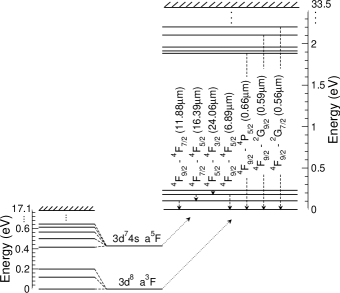
Figure 1: Important lines in the infrared and visible energy bands between levels of Co iii amongst the 3d⁷ configuration and involving the ground term ⁴F. The neighbouring system of Co ii is to the left with its split $J$ levels to indicate the photoionization process.

Index	Level	S&C	model 1	model 2	$\%$	model 3	Storey
1	3d7 a4F9/2	0.00000	0.00000	0.00000	0.0	0.00000	0.00000
2	3d7 a4F7/2	0.10430	0.10355	0.09939	4.7	0.09980	0.10216
3	3d7 a4F5/2	0.17994	0.18001	0.17255	4.1	0.17321	0.17705
4	3d7 a4F3/2	0.23145	0.23263	0.22280	3.7	0.22362	0.22838
5	3d7 a4P5/2	1.88480	2.39405	2.20436	16.9	2.19761	2.29369
6	3d7 a4P3/2	1.91285	2.42637	2.23271	16.7	2.22608	2.32904
7	3d7 a4P1/2	1.96036	2.47283	2.27875	16.2	2.27244	2.37033
8	3d7 a2G9/2	2.10496	2.39059	2.38992	13.5	2.38842	2.42773
9	3d7 a2G7/2	2.20273	2.48967	2.48250	12.7	2.48138	2.52395
10	3d7 a2P3/2	2.50385	3.16229	2.85243	13.9	2.84334	3.17809
11	3d7 a2P1/2	2.59356	3.27065	2.96428	14.3	2.95673	3.28236
12	3d7 a2H11/2	2.81696	3.18356	3.35270	19.0	3.35260	3.18478
13	3d7 a2H9/2	2.90548	3.26836	3.43116	18.1	3.43143	3.27058
14	3d7 a${}^{2}_{2}$D5/2	2.85893	3.44672	3.06277	7.1	3.04740	3.44726
15	3d7 a${}^{2}_{2}$D3/2	3.00498	3.60358	3.23140	7.5	3.21873	3.59963
16	3d7 a2F5/2	4.59002	5.51392	5.36609	16.9	5.35716	-
17	3d7 a2F7/2	4.62666	5.55837	5.40863	16.9	5.39998	-
18	3d64s a6D9/2	5.75762	6.70846	6.06849	5.4	6.20178	-
19	3d64s a6D7/2	5.82764	6.78942	6.14650	5.5	6.27925	-
20	3d64s a6D5/2	5.87876	6.84869	6.20378	5.5	6.33614	-
21	3d64s a6D3/2	5.91387	6.88947	6.24324	5.5	6.37536	-
22	3d64s a6D1/2	5.93448	6.91340	6.26643	5.6	6.39840	-
23	3d64s a4D7/2	6.90954	8.42015	7.72255	11.8	8.04998	-
24	3d64s a4D5/2	6.98946	8.51285	7.81196	11.8	8.13868	-
25	3d64s a4D3/2	7.04166	8.57368	7.87084	11.8	8.19722	-
26	3d64s a4D1/2	7.07167	8.60877	7.90480	11.8	8.23095	-
27	3d7 a${}^{2}_{1}$D3/2	-	8.67161	7.93064	-	7.96545	-
28	3d7 a${}^{2}_{1}$D5/2	-	8.61018	8.00119	-	7.89375	-
29	3d64s b4P5/2	8.79471	10.25065	9.63834	9.6	9.80974	-
30	3d64s a4H13/2	8.88014	10.00120	9.38243	5.6	9.55349	-
31	3d64s a4H11/2	8.91121	10.03198	9.41243	5.6	9.58337	-
32	3d64s a4H9/2	8.93719	10.05805	9.43786	5.6	9.60883	-
33	3d64s a4H7/2	8.96040	10.08057	9.45963	5.6	9.63075	-
34	3d64s b4P3/2	8.96926	10.46563	9.84580	9.8	10.01710	-
35	3d64s b4P1/2	9.07744	10.59439	9.97061	9.8	10.14009	-
36	3d64s b4F9/2	9.08631	10.42302	9.81043	8.0	9.98184	-
37	3d64s b4F7/2	9.11782	10.46016	9.84605	8.0	10.01692	-
38	3d64s b4F5/2	9.14093	10.49101	9.87566	8.0	10.04624	-
39	3d64s b4F3/2	9.15770	10.51540	9.89893	8.1	10.06929	-
40	3d64s a4G11/2	9.48714	10.77237	10.15994	7.1	10.33533	-
41	3d64s b2P3/2	9.52088	11.32810	10.67964	12.2	10.96474	-
42	3d64s a4G9/2	9.56180	10.85246	10.23781	7.1	10.40898	-
43	3d64s a4G7/2	9.59428	10.88642	10.27110	7.0	10.44158	-
44	3d64s b2H11/2	9.59782	11.04902	10.39701	8.3	10.67836	-
45	3d64s a4G5/2	9.60534	10.89526	10.28019	7.0	10.45125	-
46	3d64s b2P1/2	9.72461	11.57042	10.91582	12.2	11.19712	-
47	3d64s b2H9/2	9.62402	11.08283	10.42907	8.4	10.71376	-
48	3d64s b2F7/2	9.78580	11.44778	10.80218	10.4	11.08548	-
49	3d64s b2F5/2	9.84749	11.53372	10.88286	10.5	11.16801	-
50	3d64s b2G9/2	10.21175	11.83144	11.18470	9.6	11.47076	-

Table 1: Energies for the lowest 50 levels of Co iii are presented in eV relative to the ground state 3d⁷ a⁴F_9/2. S&C is from the work of Sugar & Corliss (1985). model 1, model 2, model 3 are the current results from grasp0 and the last column are the lowest 15 levels from Storey & Sochi (2016). We also present the $\%$ difference between our current model 2 and S&C in the 6th column.

As stated in the introduction, partially filled d-shell systems are difficult due to the hundreds of levels associated with a single configuration. Initially, we include three configurations, 3d⁷ and 3d⁶[4s, 4p] during the optimization process, denoted as model 1, which results in a total of 262 fine structure levels to describe the Co iii ion. The ground state of which is 3d⁷a⁴F_9/2. Next we optimize all orbitals up to 3d on the configurations from the double electron promotions, 3s², 3p² $\rightarrow$ 3d² and include in the total calculation all configurations from model 1 plus 3p⁶3d⁹ (double promotion from 3s to 3d) and 3s²3p⁴3d⁹ (double promotion from 3p to 3d). This technique can be useful as it alleviates the necessity to include numerous pseudo states into the calculation. We denote this model 2 which constitutes a total of 292 levels. Finally, by including 3d⁵[4s², 4p²] and 3d⁵4s4p, the number of levels drastically increases to 1,259 levels, and we label this as model 3.

We present in Table 1 our ab initio energy levels obtained from grasp0 in eV for the lowest lying 50 levels alongside those observed by Sugar & Corliss (1985). We also present the $\%$ difference between Sugar & Corliss (1985) and our model 2, and also provide the lowest 15 levels of Storey & Sochi (2016). Good agreement is found ($<$10% for the majority of levels) between the present model 2 and model 3 energies and those of Storey & Sochi (2016). As with other Fe-peak ions, the energy levels of the lowest-lying 3d⁷ fine-structure states are notoriously difficult to determine. The highest disparities are found for these levels when compared with Sugar & Corliss (1985), the largest being for the 3d^{7 4}F_9/2 $\rightarrow$ 3d^{7 2}H_11/2 (1-12) transition. For levels indexed above 17 the differences are at most 10-11$\%$ and for many levels by considerable less. The main problem is due to the fact that a single 3d orbital is used to describe the configuration state functions for multiple configurations of type 3d⁷ and 3d⁶4s. Similar differences were reported by Ramsbottom (2009) for the low-lying 3d⁷ fine-structure levels of Fe ii. Despite the high $\%$ differences found between these lowest levels in Table 1, overall the average $\%$ change across the 171 Sugar & Corliss (1985) J$\pi$ symmetries is a more acceptable 6.2$\%$. The differences between model 2 and model 3 are not significant enough to justify the much larger calculation, and we can also benefit by employing all 292 levels into the close-coupling wavefunction expansion of the Co iii. We therefore adopt our model 2 as the final model for the scattering calculation.

The $A$-value, or transition probability, can be calculated at this stage of the calculation. It is a direct measure of the line strength between two states of our system, and we therefore require accurate wavefunctions and energies. We can account for the discrepancy between grasp0 and Sugar & Corliss (1985) energy states by considering the following multiplicative scaling factor,

$$\Bigg{(}\frac{\Delta E^{{\rm expt}}_{ji}}{\Delta E^{{\rm theo}}_{ji}}\Bigg{)}^{\eta},$$ (2)

Here we set $\eta=3$ or $\eta=5$ for electric and magnetic dipole or quadrupole transitions between two states $j$ and $i$. It is found that these are shifted by a fraction of the recorded values. A procedure through a least squares fitting process (Cowan, 1981) is the most commonly implemented source of $A$-values for this ion stage of Cobalt (Hansen et al., 1984) to date. A total of 130 forbidden transitions within this 3d⁷ complex are reported, and are provided for comparison in Figure 2 against our results after the scaling in equation (2) has been performed. The $A$-values are presented on a logarithmic vs. logarithmic scale to incorporate the various magnitudes of results. To investigate this comparison more closely, we present in Table 2 a selection of transitions among the lowest 7 levels of Co iii. Comparisons are made between the values of (Hansen et al., 1984), the present model 2 with scaled transition energy levels and the recent results from Storey & Sochi (2016). Excellent agreement is evident for the bulk of the transitions considered with the greatest difference of $12.7\%$ occurring for the 3d⁷a⁴F_3/2 - 3d⁷a⁴P_5/2 (4-5) transition.

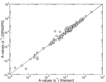
Figure 2: Present theoretical $A$-values after the scaling factors in equation (2) have been applied, plotted against the results of Hansen et al. (1984) in s^-1 on a log/log scale.

$i-j$	Fivet	Hansen	model 2	Storey
1 – 2	2.00$\times 10^{-2}$	2.00$\times 10^{-2}$	2.00$\times 10^{-2}$	2.00$\times 10^{-2}$
1 – 3	-	1.80$\times 10^{-9}$	1.75$\times 10^{-10}$	-
1 – 5	6.65$\times 10^{-2}$	4.80$\times 10^{-2}$	4.53$\times 10^{-2}$	5.55$\times 10^{-2}$
2 – 3	1.31$\times 10^{-2}$	1.30$\times 10^{-2}$	1.31$\times 10^{-2}$	1.31$\times 10^{-2}$
2 – 4	-	5.90$\times 10^{-10}$	5.70$\times 10^{-10}$	-
2 – 5	1.78$\times 10^{-2}$	1.35$\times 10^{-2}$	1.26$\times 10^{-2}$	1.51$\times 10^{-2}$
2 – 6	3.73$\times 10^{-2}$	2.70$\times 10^{-2}$	2.58$\times 10^{-2}$	3.14$\times 10^{-2}$
3 – 4	4.63$\times 10^{-2}$	4.70$\times 10^{-3}$	4.63$\times 10^{-3}$	4.63$\times 10^{-3}$
3 – 5	-	2.60$\times 10^{-3}$	2.45$\times 10^{-3}$	3.14$\times 10^{-3}$
3 – 6	2.21$\times 10^{-2}$	1.63$\times 10^{-2}$	1.50$\times 10^{-2}$	1.85$\times 10^{-2}$
3 – 7	2.73$\times 10^{-2}$	2.00$\times 10^{-2}$	1.89$\times 10^{-2}$	2.30$\times 10^{-2}$
4 – 5	-	4.00$\times 10^{-4}$	3.55$\times 10^{-4}$	-
4 – 6	-	4.40$\times 10^{-3}$	4.22$\times 10^{-1}$	5.14$\times 10^{-3}$
4 – 7	3.60$\times 10^{-2}$	2.60$\times 10^{-2}$	2.47$\times 10^{-2}$	3.02$\times 10^{-2}$
5 – 6	-	2.70$\times 10^{-4}$	2.69$\times 10^{-4}$	-
5 – 7	-	5.50$\times 10^{-9}$	5.20$\times 10^{-9}$	-
6 – 7	-	2.50$\times 10^{-3}$	2.47$\times 10^{-3}$	2.45$\times 10^{-3}$

Table 2: $A$-values from Fivet et al. (2016), Hansen et al. (1984), our current model 2 after the multiplicative scaling factors in equation (2) have been applied and results from Storey for transitions amongst the lowest 7 levels.

A much larger calculation for doubly ionized Fe-peak species has been performed recently by Fivet et al. (2016) using the same suite of codes as Hansen et al. (1984), and also by considering the computer package autostructure, (Eissner et al., 1974; Badnell, 1986), where the optimization process is carried out with a Thomas-Fermi-Dirac potential using lambda scaling parameters. Numerous doubly ionized ions of Fe, Ni and Co were considered in this publication. Single and double electron promotions out of the 3d, and also single electron promotions out of the 3s to the 5s orbital were included and comprised the basis expansion for both calculations. This is the most sophisticated and complete report for radiative rates in Co iii to date. Within the 3d⁷ complex, we vary approximately $27\%$ on average compared with both methods of Fivet et al. (2016).

2.2 The $R$-matrix method

To extend this problem to include interactions with photons and electrons, we consider the $R$-matrix method. A general overview of the theory can be found in Burke (2011). The theory was developed to perform electron scattering by Burke et al. (1971) and extended for photoionization by Burke & Taylor (1975).

These calculations can be performed using a non orthogonal B-spline basis set approach (Zatsarinny & Froese Fischer, 2000; Zatsarinny & Bartschat, 2004), intermediate-coupling frame transformation methods (Griffin et al., 1998) and one-body perturbation corrections to the non-relativistic Hamiltonian via the Breit-Pauli operators (Scott & Burke, 1980) to name a few. In this paper, we consider the Dirac-Atomic $R$-matrix codes (darc) to accurately include important relativistic effects through the Dirac Hamiltonian in equation (1) for this mid to heavy species ion. The wavefunctions obtained from grasp0 are formatted suitable for inclusion into darc. Validity of these methods between the outlined theoretical approaches are always important, and enhance the robustness of the techniques carried out as seen in Tyndall et al. (2016) for Ar⁺ and Fernández-Menchero et al. (2015) for Al⁹⁺. Therefore, it is possible to benchmark sophisticated experimental techniques against theory (Müller et al., 2009; Gharaibeh et al., 2011).

2.3 Photoionization

The photoionization process is described by,

$$h\nu+{\rm Co}^{+}~{}\{{\rm 3d}^{8}{\rm a}^{3}{\rm F}^{{\rm e}}_{J},{\rm 3d}^{7}{\rm 4s~{}a}^{5}{\rm F}^{{\rm e}}_{J}\}\rightarrow{\rm Co}^{2+}+e^{{\rm-}}$$ (3)

where a photon leads to the ionization of an electon directly, or via a Rydberg resonance. The process in equation (3) can be formally calculated as,

$$\sigma^{{\rm p}}_{i\rightarrow j}=\frac{4\pi a_{0}^{2}\alpha\omega}{3g_{i}}\sum(\Psi_{j}||\mathbf{D}||\Psi_{i})$$

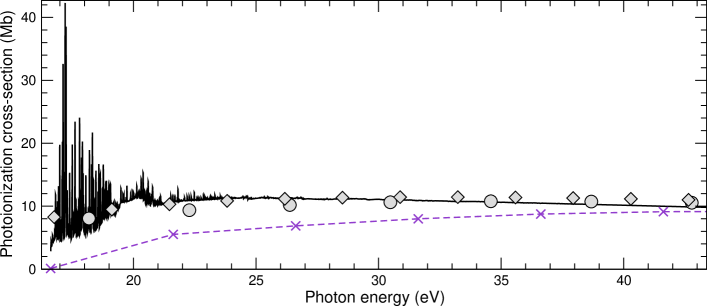
Figure 3: Photoionization cross-sections in Mb against the photon energy in eV. The solid black curve is the total initial ground state, statistically weighted 3d^{8 3}F to all allowed dipole final states. The crosses are results from Reilman & Manson (1979), the diamonds are from Verner et al. (1993), and finally the circles are those from the distorted wave calculation. (Fontes et al., 2015)

for initial and final scattering wavefunctions subject to the total dipole contribution. $\omega=h\nu$ is the photon energy or $\omega\rightarrow\omega^{-1}$ when considering the velocity operator, $\mathbf{D}$. $\alpha$ is the fine structure constant, $a_{0}$ is the bohr radius and $g_{i}$ is the statistical weight of the initial state wavefunction. The summation is then carried out over all dipole-allowed transitions. The total wavefunctions $\Psi$ are obtained from the momenta couplings with those wavefunctions obtained in Section 2.1. We represent these $\sigma^{{\rm p}}$ in units of Mb ($\equiv 10^{-18}$cm²) throughout this work.

The transitions of interest are calculated within the lowest eight fine-structure levels of Co ii pertaining to the two $LS\pi$ states as noted in equation (3). We also maintain a closed 3p⁶ core and are only concerned with low energy transitions above threshold. Therefore, all even and odd allowed dipole symmetries up to $J=6$ are calculated subject to the selection rules.

Index	Level	Pickering	Current	$\Delta$
1	3p63d8 a3F4	-17.0844	-16.6232	0.46
2	3p63d8 a3F3	-16.9666	-16.5004	0.47
3	3p63d8 a3F2	-16.8864	-16.4159	0.47
4	3p63d7(4F)4s a5F5	-16.6690	-16.3531	0.32
5	3p63d7(4F)4s a5F4	-16.5849	-16.2694	0.32
6	3p63d7(4F)4s a5F3	-16.5189	-16.2031	0.32
7	3p63d7(4F)4s a5F2	-16.4707	-16.1544	0.32
8	3p63d7(4F)4s a5F1	-16.4391	-16.1224	0.32

Table 3: Bound state energies of the lowest eight states of Co ii relative to the ground state 3d⁷ a³F_9/2 of Co iii compared with the relative energies of Pickering et al. (1998), labelled as Pickering.

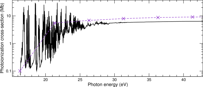
Figure 4: Photoionization cross-sections in Mb against the photon energy in eV. The solid black curve is the photoionization, statistically averaged levels of 3d⁷4s ⁵F to all allowed dipole final states. The crosses are results from Reilman & Manson (1979).

2.4 Electron-impact excitation

The collision strength between an initial state $i$ and final state $j$ can be obtained from the cross section, $\sigma^{e}$,

$$\Omega_{i\rightarrow j}=\frac{g_{i}k_{i}^{2}}{\pi a_{0}^{2}}\sigma^{e}_{j\rightarrow i}.$$ (4)

These collision strengths represent a detailed spectrum, complete with the already mentioned autoionizing states. To present the results in a more concise format, we assume a Maxwellian distribution of the colliding electron velocities. We define the effective collision strength as

$$\Upsilon_{i\rightarrow j}=\int^{\infty}_{0}\Omega_{i\rightarrow j}e^{-\epsilon_{f}/kT}d\Big{(}\frac{\epsilon_{f}}{kT}\Big{)},$$ (5)

where $\epsilon_{f}$ is the ejected energy of the electron, $3,800\leq T\leq 40,000$ in K, and $k=8.617\times 10^{-5}$ eV/K is Boltzmanns constant. Each $\Upsilon_{i\rightarrow j}$ is calculated for 11 electron temperatures.

We calculate the main contribution to the collision strength defined in equation (4) from the partial waves up to $J=13$ of both even and odd parity. These are obtained by considering appropriate total multiplicity and orbital angular momentum partial waves. However, in order to converge transitions at higher energies, we explicitly calculate partial waves up to $J=38$ and use top-up procedures outlined in Burgess & Tully (1992) to account for further contribution to the total cross-section

3 Results

As mentioned previously, the photoionization of Co ii and electron-impact excitation of Co iii rely on an accurate description of the Co iii wavefunctions. We are able to retain consistency throughout the calculation, and the fundamental $R$-matrix conditions apply to both processes. We select a total of 14 continuum basis orbitals per angular momenta to describe the scattered electron. The $R$-matrix boundary is then set at 10.88 a.u. in order to enclose the radial extent of the 4p orbital. To make comparisons between observation, the target thresholds obtained in Table 1 have been shifted to those of Sugar & Corliss (1985).

3.1 Photoionization

In this section, we detail our results from the photoionization process described by equation (3). There is minimal atomic data for this interaction in the literature as only the total ground state transition exists. The first compilation is from Reilman & Manson (1979), using Hartree-Slater wavefunctions from a Central field potential. Second, and more recently, Verner et al. (1993) have calculated cross-sections using the Hartree-Dirac-Slater potential and then applying an analytic fitting procedure. Recently, the Los Alamos suite of codes by Fontes et al. (2015) have been used to obtain results by a distorted wave method. For this we look at the photoionization of a 3d electron into the configuration averaged final states. To carefully resolve these spectra, we have employed a total of 200,000 equally spaced energy points over a photoelectron energy range of 20 eV. This ensures the high $nl$ Rydberg resonant states are properly delineated.

The initial bound states that are required, corresponding to the left hand side of equation (3) are calculated first. In Table 3 we present the energies relative to the ground state 3d⁷ a³F_9/2 of Co iii from our current $R$-matrix results and compare with those of Pickering et al. (1998). We deviate $\approx 0.47$ eV for the 3d⁸ and $\approx 0.32$ eV for the 3d⁷(⁴F)4s. Despite these discrepancies good agreement is evident for the splitting between all eight fine-structure levels.

In Figure 3 we present the photoionization cross-section representing the statistically weighted initial state 3d⁸ a³F to all allowed final states. The results in this figure have been convoluted with a 10 meV Gaussian profile at full-width half-maximum to better compare with experiment. We directly compare here with the results of all three previously mentioned theoretical methods (Reilman & Manson, 1979; Verner et al., 1993; Fontes et al., 2015). These methods do not include autoionization states and therefore only background cross-sections are presented. It is clear however that the results are in excellent agreement, with only Reilman & Manson (1979) reaching factors of two or more difference in the $<20$ eV region. As over 200 eigenenergies obtained from grasp0 are $<$ 28 eV of photon energy, this above threshold region is dominated by multiple Rydberg resonances series converging onto these states.

The second statistically weighted bound state a⁵F of Co ii is from the configuration 3d⁷4s. In Figure 4 we present the total photoionization cross-section for this metastable level and compare with the earlier work of Reilman & Manson (1979). This cross-section is weighted as a consequence of its five fine-structure split levels $1<J<5$. Again, the photoionization of the 3d electron is favourable, so we expect the majority of the spectrum to be accounted for from the 3d⁶4s target states, which are accessible at 5.75762 eV above the ionization threshold. Good agreement is found between the two calculations for the background cross section, particularly in the higher photon energy range above 25 eV.

3.2 Electron-impact excitation

The procedures outlined in Section 2.4 are now applied to obtain accurate collision strengths and the corresponding effective collision strengths describing the electron-impact excitation of Co iii. There has been work carried out recently on both singly ionized Co ii (Storey et al., 2015) and also Co iii (Storey & Sochi, 2016). The work of Storey & Sochi (2016) is similar to our current evaluation, but differences are evident in the method considered. Their basis set has been optimized using autostructure , and also includes a $4\bar{d}$ orbital plus additional configuration interaction. However, only a total of 109 fine structure levels have been included in the close coupling target representation. The semi-relativistic Breit-Pauli $R$-matrix approach was considered during the scattering calculation.

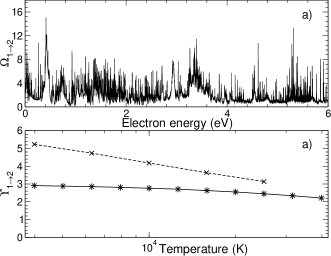
(a)

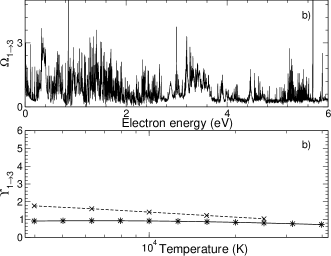
(b)

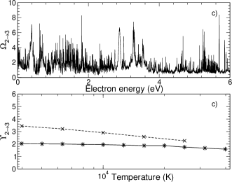
(c)

Figure 5: The collision strengths, a) $\Omega_{1\rightarrow 2}$, b) $\Omega_{1\rightarrow 3}$ and c) $\Omega_{2\rightarrow 3}$ presented as a function of electron energy in eV. Also presented are the corresponding effective collision strengths as a function of temperature in K. Solid black lines with stars are the current data set and the dashed line with crosses represent the results from Storey & Sochi (2016).

It is necessary to obtain a level of convergence in the spectra of collision strengths by applying a mesh with incremental step sizes in electron energy until convergence is achieved. Initially 5,000 equally spaced energy points were considered and it was found by the time we had reached 40,000 energy points, the $\Upsilon$s had converged for the forbidden transitions among the 292 levels. To extend the energy region we incorporated an additional coarse mesh above the last valence threshold. Due to the long range nature of the Coulomb potential further contributions to the collision strengths arise from the higher partial waves, particularly for the dipole allowed lines. We compute these additional contributions using the Burgess & Tully (1992) sum rule as well as a geomteric series for the long-range non-dipole transitions. Hence converged total collision strengths were accurately generated for all 42,486 transitions among the 292 fine-structure levels included in the collision calculation. The corresponding effective collision strengths were obtained by averaging these finely resolved collision strengths over a Maxwellian distribution of electron velocities for electron temperatures ranging from 3,800 to 40,000 K.

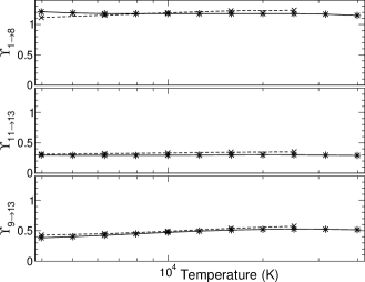
Figure 6: The effective collision strengths, $\Upsilon_{1\rightarrow 8}$ (top), $\Upsilon_{11\rightarrow 13}$ (middle) and $\Upsilon_{9\rightarrow 13}$ (bottom), presented as a function of temperature in K (bottom). Solid black lines with stars are the current data set and the dashed line with crosses represent the results from (Storey & Sochi, 2016).

We present in Figure 5 the resulting collision strengths and effective collision strengths for a selection of the forbidden near infrared transitions involving the fine-structure split levels of the ⁴F ground state of Co iii. Panel (a) represents transition from level 1$\rightarrow$ 2, panel (b) $1\rightarrow 3$, and panel (c) $2\rightarrow 3$. The collision strength is strongest here for the $\Omega_{1\rightarrow 2}$ transition due to the $\Delta J=0$ partial wave. Comparison of the effective collision strengths are made for each transition with the work of Storey & Sochi (2016) and good agreement is found for all temperatures above 10,000 K. For temperatures below this value the two calculations deviate somewhat, most probably due to the differing resonance profiles converging onto differing threshold positions. The present calculation has shifted the thresholds to lie in their exact observed positions listed in Table 1. In Figure 6 we present the effective collision strengths for some higher lying transitions, the 3d^{7 4}F_9/2 - 3d^{7 2}G_9/2 (1 $\rightarrow$ 8), 3d^{7 2}P_1/2 - 3d^{7 2}H_9/2 (11 $\rightarrow$ 13) and 3d^{7 2}G_7/2 - 3d^{7 2}H_9/2 (9 $\rightarrow$ 13). Excellent agreement is evident for all three transitions when a comparison is made with the data of Storey & Sochi (2016) across all temperatures where a comparison is possible. The collision strengths and effective collision strengths for all 42,486 forbidden and allowed lines are available from the authors on request but we present in Table 4 the effective collision strengths for all transitions among the lowest 11 3d⁷ fine-structure levels across nine temperatures of astrophysical importance.

3.3 Line ratios

Combining the electron-impact excitation rates with the decay rates ($A$-values), it is possible to investigate important infrared and visible line ratios. For simplicity and purpose of this study, we neglect the recombination and reverse ionization process from the neighbouring ion stages and focus on the populating mechanisms solely of Co iii. Assuming local thermal equilibrium and detailed balance, we can derive the collisional radiative modelling approach detailed in (Griffin et al., 1997). We can therefore investigate select transitions that have been suggested as temperature or density diagnostics. We define the line ratio as

$$\mathcal{R}=\frac{I_{j\rightarrow i}}{I_{k\rightarrow m}}=\frac{N_{j}A_{j\rightarrow i}}{N_{k}A_{k\rightarrow m}}\frac{\lambda_{mk}}{\lambda_{ij}},$$

where the populations of the $n^{th}$ level in terms of the ground state are given by $N_{n}$ and the decay rates are the results from Section 2.1.

Figure 7 depicts the results of the line ratio [0.66$\mu$m]/[0.69$\mu$m] which corresponds to the transitions,

$$\frac{I_{5\rightarrow 1}}{I_{6\rightarrow 2}}=\frac{3\rm{d}^{7}~{}\rm{a}^{4}\rm{P}_{5/2}\rightarrow 3\rm{d}^{7}~{}\rm{a}^{4}\rm{F}_{9/2}}{3\rm{d}^{7}~{}\rm{a}^{4}\rm{P}_{3/2}\rightarrow 3\rm{d}^{7}~{}\rm{a}^{4}\rm{F}_{7/2}},$$

as a function of electron density for particular temperatures. The dashed line provides the lowest temperature, $T=3,980$K, with increasing $T$ to $T=5,010$K, $T=6,310$K and $T=7,940$K. The line ratio is constant for densities $N_{e}<10^{4}$ cm^-3 and also $N_{e}>10^{7}$ cm^-3 for the temperatures considered. This could be considered a useful diagnostic for densities in the range of $10^{4}$ cm^-3 $<N_{e}<3\times 10^{5}$ cm^-3 where it remains constant for increasing temperatures before it reaches its minimum $\approx 5\times 10^{5}$ cm^-3

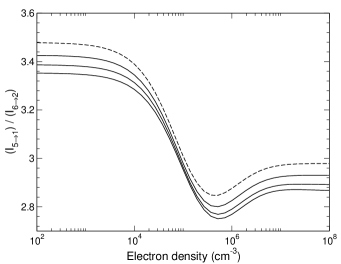
Figure 7: The line ratio [0.66$\mu$m]/[0.69$\mu$m] as a function of electron density (cm^-3). The dashed curve is the lowest temperature, $T=3,980$K. The remaining solid black curves are for temperatures $T=5,010$K, $T=6,310$K, and $T=7,940$K for decreasing line ratio.

Next we consider lines suggested by Ruiz-Lapuente (1995), (around the wavelength region 6,000 - 6,500 Å) to be applied as density diagnostics. At 10,000 K, we can see the photon emissivity coefficients of the $8\rightarrow 1$ and $8\rightarrow 2$ lines becomes more dominant for increasing temperatures, and are in the ideal wavelength region. Telesco et al. (2015) also suggests the $2\rightarrow 1$, 11.88$\mu$m as a useful diagnostic line. We finally present the results of three line ratios ,

$$\frac{I_{2\rightarrow 1}[11.88\mu m]}{I_{5\rightarrow 1}[0.66\mu m]}=\frac{3\rm{d}^{7}~{}\rm{a}^{4}\rm{F}_{7/2}\rightarrow 3\rm{d}^{7}~{}\rm{a}^{4}\rm{F}_{9/2}}{3\rm{d}^{7}~{}\rm{a}^{4}\rm{P}_{5/2}\rightarrow 3\rm{d}^{7}~{}\rm{a}^{4}\rm{F}_{9/2}},$$

$$\frac{I_{2\rightarrow 1}[11.88\mu m]}{I_{5\rightarrow 1}[0.59\mu m]}=\frac{3\rm{d}^{7}~{}\rm{a}^{4}\rm{F}_{7/2}\rightarrow 3\rm{d}^{7}~{}\rm{a}^{4}\rm{F}_{9/2}}{3\rm{d}^{7}~{}\rm{a}^{2}\rm{G}_{9/2}\rightarrow 3\rm{d}^{7}~{}\rm{a}^{4}\rm{F}_{9/2}},$$

$$\frac{I_{2\rightarrow 1}[11.88\mu m]}{I_{5\rightarrow 1}[0.62\mu m]}=\frac{3\rm{d}^{7}~{}\rm{a}^{4}\rm{F}_{7/2}\rightarrow 3\rm{d}^{7}~{}\rm{a}^{4}\rm{F}_{9/2}}{3\rm{d}^{7}~{}\rm{a}^{2}\rm{G}_{9/2}\rightarrow 3\rm{d}^{7}~{}\rm{a}^{4}\rm{F}_{7/2}},$$

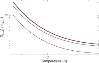
(a)

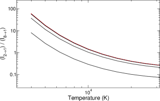
(b)

(c)

Figure 8: The line ratio [11.88$\mu$m]/[0.66$\mu$m] (top), [11.88$\mu$m]/[0.59$\mu$m] (middle), and [11.88$\mu$m]/[0.62$\mu$m] (bottom) as a function of electron temperature (K). The red, dashed curve is the lowest density, $N_{e}=10^{2}$ cm^-3. The remaining solid black curves are for temperatures $N_{e}=10^{3}$ cm^-3, $N_{e}=10^{4}$ cm^-3, $N_{e}=10^{5}$ cm^-3, and $N_{e}=10^{6}$ cm^-3 for decreasing line ratio.

We plot Figure 8 as a function of electron temperature for all three line ratios. The red dashed curve is the lowest electron density in each subfigure, $N_{e}=10^{2}$ cm^-3, and the remaining solid curves correspond to $N_{e}=10^{3}$ cm^-3, $N_{e}=10^{4}$ cm^-3, $N_{e}=10^{5}$ cm^-3, and $N_{e}=10^{6}$ cm^-3. Each line ratio is a varying function of increasing temperature across the range of interest. The line ratios for three lowest densities are generally unchanged, and therefore they provide useful diagnostics for this density range. As $N_{e}=10^{5}$ cm^-3 and beyond, the line ratio begins to diverge, and becomes constant for even larger densities.

4 Conclusion

In this paper we present an extensive set of atomic data for the photoionization of Co ii and the electron-impact excitation of Co iii. Initially we have exploited the computer code grasp0 to obtain a description of the atomic wavefunctions and generate energy levels for the 292 fine-structure bound target states and the corresponding $A$-values for transitions between these levels. Furthermore, the darc computer package has been employed to extend the problem to include photon and electron interactions. We present statistically weighted, level-resolved ground and metastable photoionization cross-sections for the Co ii ion as well as collision strengths and Maxwellian averaged effective collision strengths describing the electron-impact excitation of the Co iii ion. Comparisons are made with other works where possible and good agreement is found where a comparison is available. The reliability of the atomic data presented has been rigorously tested through a variety of means, such as the sophistication of the current calculations where great care has been taken to ensure the inclusion of important correlation and configuration-interaction in the wavefunction expansions. In addition the complex resonance structures in the cross sections (photoionization and excitation) have been accurately resolved through a series of calculations incorporating mesh sizes with finer and finer energy increments. A proper consideration was also taken of the contributions from the high partial waves to ensure convergence of the collision strengths for the allowed transitions in particular (which are not presented in this work). A conclusive assessment of the accuracy of the presented Maxwellian averaged collision strengths will necessarily come from any subsequent astrophysical or diagnostic application. In Section 3.3 the electron-impact excitation rates were combined with the decay rates ($A$-values) to investigate important infrared and visible line ratios. During this process we were able to identify useful transitions that could be used as temperature and/or density sensitive diagnostic lines.

		log $T$ (K)
$i$	$j$	3.6	3.7	3.8	3.9	4	4.1	4.2	4.3	4.4
1	2	$2.92^{+00}$	$2.90^{+00}$	$2.86^{+00}$	$2.82^{+00}$	$2.77^{+00}$	$2.70^{+00}$	$2.63^{+00}$	$2.54^{+00}$	$2.44^{+00}$
1	3	$9.24^{-01}$	$9.36^{-01}$	$9.41^{-01}$	$9.37^{-01}$	$9.26^{-01}$	$9.06^{-01}$	$8.79^{-01}$	$8.45^{-01}$	$8.06^{-01}$
2	3	$2.02^{+00}$	$2.01^{+00}$	$1.99^{+00}$	$1.97^{+00}$	$1.94^{+00}$	$1.91^{+00}$	$1.86^{+00}$	$1.81^{+00}$	$1.74^{+00}$
1	4	$3.17^{-01}$	$3.23^{-01}$	$3.26^{-01}$	$3.25^{-01}$	$3.21^{-01}$	$3.13^{-01}$	$3.03^{-01}$	$2.90^{-01}$	$2.75^{-01}$
2	4	$7.46^{-01}$	$7.65^{-01}$	$7.77^{-01}$	$7.80^{-01}$	$7.76^{-01}$	$7.64^{-01}$	$7.43^{-01}$	$7.17^{-01}$	$6.85^{-01}$
3	4	$1.42^{+00}$	$1.42^{+00}$	$1.42^{+00}$	$1.42^{+00}$	$1.40^{+00}$	$1.39^{+00}$	$1.36^{+00}$	$1.32^{+00}$	$1.28^{+00}$
1	5	$1.16^{+00}$	$1.16^{+00}$	$1.17^{+00}$	$1.19^{+00}$	$1.20^{+00}$	$1.21^{+00}$	$1.21^{+00}$	$1.20^{+00}$	$1.19^{+00}$
2	5	$8.11^{-01}$	$8.03^{-01}$	$8.02^{-01}$	$8.07^{-01}$	$8.13^{-01}$	$8.17^{-01}$	$8.15^{-01}$	$8.05^{-01}$	$7.89^{-01}$
3	5	$5.72^{-01}$	$5.60^{-01}$	$5.53^{-01}$	$5.51^{-01}$	$5.50^{-01}$	$5.48^{-01}$	$5.43^{-01}$	$5.33^{-01}$	$5.19^{-01}$
4	5	$3.68^{-01}$	$3.51^{-01}$	$3.37^{-01}$	$3.27^{-01}$	$3.20^{-01}$	$3.13^{-01}$	$3.06^{-01}$	$2.98^{-01}$	$2.88^{-01}$
1	6	$4.84^{-01}$	$4.82^{-01}$	$4.84^{-01}$	$4.90^{-01}$	$4.95^{-01}$	$4.98^{-01}$	$4.97^{-01}$	$4.91^{-01}$	$4.82^{-01}$
2	6	$5.54^{-01}$	$5.52^{-01}$	$5.53^{-01}$	$5.56^{-01}$	$5.60^{-01}$	$5.61^{-01}$	$5.58^{-01}$	$5.52^{-01}$	$5.41^{-01}$
3	6	$4.55^{-01}$	$4.51^{-01}$	$4.51^{-01}$	$4.54^{-01}$	$4.57^{-01}$	$4.59^{-01}$	$4.57^{-01}$	$4.52^{-01}$	$4.44^{-01}$
4	6	$2.92^{-01}$	$2.88^{-01}$	$2.89^{-01}$	$2.92^{-01}$	$2.96^{-01}$	$3.00^{-01}$	$3.02^{-01}$	$3.00^{-01}$	$2.96^{-01}$
5	6	$6.14^{-01}$	$6.15^{-01}$	$6.21^{-01}$	$6.31^{-01}$	$6.44^{-01}$	$6.59^{-01}$	$6.73^{-01}$	$6.82^{-01}$	$6.87^{-01}$
1	7	$1.86^{-01}$	$1.85^{-01}$	$1.85^{-01}$	$1.86^{-01}$	$1.87^{-01}$	$1.86^{-01}$	$1.84^{-01}$	$1.81^{-01}$	$1.76^{-01}$
2	7	$2.03^{-01}$	$2.03^{-01}$	$2.06^{-01}$	$2.10^{-01}$	$2.15^{-01}$	$2.18^{-01}$	$2.19^{-01}$	$2.18^{-01}$	$2.14^{-01}$
3	7	$2.34^{-01}$	$2.36^{-01}$	$2.39^{-01}$	$2.43^{-01}$	$2.48^{-01}$	$2.51^{-01}$	$2.53^{-01}$	$2.52^{-01}$	$2.48^{-01}$
4	7	$2.19^{-01}$	$2.20^{-01}$	$2.22^{-01}$	$2.26^{-01}$	$2.29^{-01}$	$2.31^{-01}$	$2.32^{-01}$	$2.31^{-01}$	$2.28^{-01}$
5	7	$2.43^{-01}$	$2.45^{-01}$	$2.49^{-01}$	$2.56^{-01}$	$2.65^{-01}$	$2.75^{-01}$	$2.85^{-01}$	$2.93^{-01}$	$2.98^{-01}$
6	7	$2.73^{-01}$	$2.72^{-01}$	$2.72^{-01}$	$2.74^{-01}$	$2.76^{-01}$	$2.79^{-01}$	$2.81^{-01}$	$2.83^{-01}$	$2.82^{-01}$
1	8	$1.22^{+00}$	$1.20^{+00}$	$1.19^{+00}$	$1.19^{+00}$	$1.19^{+00}$	$1.19^{+00}$	$1.19^{+00}$	$1.19^{+00}$	$1.18^{+00}$
2	8	$7.27^{-01}$	$7.14^{-01}$	$7.06^{-01}$	$7.02^{-01}$	$6.99^{-01}$	$6.98^{-01}$	$6.96^{-01}$	$6.92^{-01}$	$6.86^{-01}$
3	8	$3.85^{-01}$	$3.76^{-01}$	$3.70^{-01}$	$3.65^{-01}$	$3.62^{-01}$	$3.59^{-01}$	$3.55^{-01}$	$3.51^{-01}$	$3.45^{-01}$
4	8	$1.75^{-01}$	$1.69^{-01}$	$1.65^{-01}$	$1.60^{-01}$	$1.57^{-01}$	$1.53^{-01}$	$1.50^{-01}$	$1.46^{-01}$	$1.43^{-01}$
5	8	$3.24^{-01}$	$3.18^{-01}$	$3.11^{-01}$	$3.07^{-01}$	$3.04^{-01}$	$3.02^{-01}$	$3.01^{-01}$	$3.00^{-01}$	$2.98^{-01}$
6	8	$1.56^{-01}$	$1.51^{-01}$	$1.47^{-01}$	$1.43^{-01}$	$1.41^{-01}$	$1.40^{-01}$	$1.39^{-01}$	$1.38^{-01}$	$1.37^{-01}$
7	8	$5.48^{-02}$	$5.20^{-02}$	$4.93^{-02}$	$4.70^{-02}$	$4.51^{-02}$	$4.36^{-02}$	$4.24^{-02}$	$4.14^{-02}$	$4.03^{-02}$
1	9	$3.16^{-01}$	$3.10^{-01}$	$3.06^{-01}$	$3.05^{-01}$	$3.05^{-01}$	$3.04^{-01}$	$3.03^{-01}$	$3.01^{-01}$	$2.97^{-01}$
2	9	$5.02^{-01}$	$4.99^{-01}$	$4.99^{-01}$	$5.01^{-01}$	$5.05^{-01}$	$5.08^{-01}$	$5.11^{-01}$	$5.12^{-01}$	$5.10^{-01}$
3	9	$5.33^{-01}$	$5.29^{-01}$	$5.29^{-01}$	$5.31^{-01}$	$5.34^{-01}$	$5.37^{-01}$	$5.40^{-01}$	$5.41^{-01}$	$5.39^{-01}$
4	9	$4.29^{-01}$	$4.27^{-01}$	$4.26^{-01}$	$4.27^{-01}$	$4.29^{-01}$	$4.32^{-01}$	$4.33^{-01}$	$4.34^{-01}$	$4.32^{-01}$
5	9	$1.53^{-01}$	$1.46^{-01}$	$1.41^{-01}$	$1.37^{-01}$	$1.36^{-01}$	$1.36^{-01}$	$1.36^{-01}$	$1.37^{-01}$	$1.36^{-01}$
6	9	$1.72^{-01}$	$1.66^{-01}$	$1.62^{-01}$	$1.58^{-01}$	$1.56^{-01}$	$1.56^{-01}$	$1.55^{-01}$	$1.55^{-01}$	$1.55^{-01}$
7	9	$1.09^{-01}$	$1.06^{-01}$	$1.04^{-01}$	$1.02^{-01}$	$1.01^{-01}$	$9.99^{-02}$	$9.95^{-02}$	$9.92^{-02}$	$9.86^{-02}$
8	9	$1.29^{+00}$	$1.27^{+00}$	$1.26^{+00}$	$1.26^{+00}$	$1.27^{+00}$	$1.28^{+00}$	$1.29^{+00}$	$1.29^{+00}$	$1.28^{+00}$
1	10	$3.06^{-01}$	$3.04^{-01}$	$3.04^{-01}$	$3.03^{-01}$	$3.03^{-01}$	$3.02^{-01}$	$3.00^{-01}$	$2.99^{-01}$	$2.97^{-01}$
2	10	$2.76^{-01}$	$2.79^{-01}$	$2.82^{-01}$	$2.86^{-01}$	$2.88^{-01}$	$2.89^{-01}$	$2.87^{-01}$	$2.83^{-01}$	$2.78^{-01}$
3	10	$2.05^{-01}$	$2.09^{-01}$	$2.13^{-01}$	$2.18^{-01}$	$2.21^{-01}$	$2.21^{-01}$	$2.20^{-01}$	$2.16^{-01}$	$2.10^{-01}$
4	10	$1.29^{-01}$	$1.32^{-01}$	$1.36^{-01}$	$1.40^{-01}$	$1.43^{-01}$	$1.43^{-01}$	$1.42^{-01}$	$1.39^{-01}$	$1.34^{-01}$
5	10	$2.85^{-01}$	$2.84^{-01}$	$2.86^{-01}$	$2.89^{-01}$	$2.92^{-01}$	$2.95^{-01}$	$2.95^{-01}$	$2.93^{-01}$	$2.89^{-01}$
6	10	$2.29^{-01}$	$2.27^{-01}$	$2.27^{-01}$	$2.29^{-01}$	$2.31^{-01}$	$2.32^{-01}$	$2.31^{-01}$	$2.29^{-01}$	$2.25^{-01}$
7	10	$9.14^{-02}$	$9.23^{-02}$	$9.39^{-02}$	$9.56^{-02}$	$9.69^{-02}$	$9.75^{-02}$	$9.72^{-02}$	$9.60^{-02}$	$9.40^{-02}$
8	10	$4.12^{-01}$	$4.06^{-01}$	$4.01^{-01}$	$3.99^{-01}$	$3.99^{-01}$	$4.00^{-01}$	$4.03^{-01}$	$4.07^{-01}$	$4.09^{-01}$
9	10	$3.20^{-01}$	$3.17^{-01}$	$3.17^{-01}$	$3.20^{-01}$	$3.26^{-01}$	$3.34^{-01}$	$3.42^{-01}$	$3.47^{-01}$	$3.50^{-01}$
1	11	$8.09^{-02}$	$8.03^{-02}$	$8.01^{-02}$	$8.02^{-02}$	$8.05^{-02}$	$8.08^{-02}$	$8.09^{-02}$	$8.08^{-02}$	$8.03^{-02}$
2	11	$1.09^{-01}$	$1.10^{-01}$	$1.11^{-01}$	$1.11^{-01}$	$1.12^{-01}$	$1.12^{-01}$	$1.12^{-01}$	$1.11^{-01}$	$1.09^{-01}$
3	11	$1.16^{-01}$	$1.19^{-01}$	$1.22^{-01}$	$1.26^{-01}$	$1.28^{-01}$	$1.29^{-01}$	$1.28^{-01}$	$1.27^{-01}$	$1.24^{-01}$
4	11	$9.23^{-02}$	$9.71^{-02}$	$1.02^{-01}$	$1.07^{-01}$	$1.11^{-01}$	$1.13^{-01}$	$1.13^{-01}$	$1.11^{-01}$	$1.08^{-01}$
5	11	$7.49^{-02}$	$7.54^{-02}$	$7.66^{-02}$	$7.83^{-02}$	$8.00^{-02}$	$8.14^{-02}$	$8.23^{-02}$	$8.23^{-02}$	$8.14^{-02}$
6	11	$8.77^{-02}$	$8.98^{-02}$	$9.27^{-02}$	$9.61^{-02}$	$9.93^{-02}$	$1.02^{-01}$	$1.04^{-01}$	$1.04^{-01}$	$1.03^{-01}$
7	11	$6.77^{-02}$	$6.93^{-02}$	$7.18^{-02}$	$7.45^{-02}$	$7.70^{-02}$	$7.88^{-02}$	$7.96^{-02}$	$7.94^{-02}$	$7.81^{-02}$
8	11	$1.98^{-01}$	$1.90^{-01}$	$1.85^{-01}$	$1.81^{-01}$	$1.79^{-01}$	$1.78^{-01}$	$1.78^{-01}$	$1.79^{-01}$	$1.79^{-01}$
9	11	$2.06^{-01}$	$2.01^{-01}$	$1.99^{-01}$	$1.99^{-01}$	$2.00^{-01}$	$2.03^{-01}$	$2.07^{-01}$	$2.11^{-01}$	$2.14^{-01}$
10	11	$3.32^{-01}$	$3.24^{-01}$	$3.19^{-01}$	$3.17^{-01}$	$3.17^{-01}$	$3.17^{-01}$	$3.16^{-01}$	$3.14^{-01}$	$3.09^{-01}$

Table 4: Effective collision strengths as defined by equation (5) are presented between an upper ($j$) and lower state ($i$), across a range of 9 temperatures (K), 3,800K $<T<$ 25,100K.

References

- Aggarwal et al. (2015) Aggarwal K. M., Bogdanovich P., Karpuškienė R., Keenan F. P., Kisielius R., Stancalie V., 2015, ArXiv e-prints
- Badnell (1986) Badnell N. R., 1986, J. Phys. B: At. Mol. Phys., 19, 3827
- Bautista et al. (2015) Bautista M. A., Fivet V., Ballance C., Quinet P., Ferland G., Mendoza C., Kallman T. R., 2015, ApJ, 808, 174
- Bergemann et al. (2010) Bergemann M., Pickering J. C., Gehren T., 2010, MNRAS, 401, 1334
- Burgess & Tully (1992) Burgess A., Tully J. A., 1992, AAP, 254, 436
- Burke (2011) Burke P. G., 2011, R-Matrix Theory of Atomic Collisions. Springer-Verlag: Berlin Heidelberg
- Burke et al. (1971) Burke P. G., Hibbert A., Robb W. D., 1971, J. Phys. B: At. Mol. Phys., 4, 153
- Burke & Taylor (1975) Burke P. G., Taylor K. T., 1975, J. Phys. B: At. Mol. Phys., 8, 2620
- Cardon et al. (1982) Cardon B. L., Smith P. L., Scalo J. M., Testerman L., Whaling W., 1982, ApJ, 260, 395
- Cowan (1981) Cowan R. D., 1981, The theory of atomic structure and spectra. Berkeley: Univ. California Press
- Dessart et al. (2014) Dessart L., Hillier D. J., Blondin S., Khokhlov A., 2014, MNRAS, 441, 3249
- Diamond et al. (2015) Diamond T. R., Hoeflich P., Gerardy C. L., 2015, ApJ, 806, 107
- Dworetsky (1982) Dworetsky M. M., 1982, Observatory, 102, 138
- Dworetsky et al. (1980) Dworetsky M. M., Trueman M. R. G., Stickland D. J., 1980, AAP, 85, 138
- Eissner et al. (1974) Eissner W., Jones M., Nussbaumer H., 1974, Computer Physics Communications, 8, 270
- Federman et al. (1993) Federman S. R., Sheffer Y., Lambert D. L., Gilliland R. L., 1993, ApJ, 413, L51
- Fernández-Menchero et al. (2015) Fernández-Menchero L., Del Zanna G., Badnell N. R., 2015, MNRAS, 450, 4174
- Fivet et al. (2016) Fivet V., Quinet P., Bautista M. A., 2016, AAP, 585, A121
- Fontes et al. (2015) Fontes C. J., Zhang H. L., Abdallah Jr. J., Clark R. E. H., Kilcrease D. P., Colgan J., Cunningham R. T., Hakel P., Magee N. H., Sherrill M. E., 2015, J. Phys. B: At. Mol. Phys., 48, 144014
- Gerardy et al. (2007) Gerardy C. L., Meikle W. P. S., Kotak R., Höflich P., Farrah D., Filippenko A. V., Foley R. J., Lundqvist P., Mattila S., Pozzo M., Sollerman J., Van Dyk S. D., Wheeler J. C., 2007, ApJ, 661, 995
- Gharaibeh et al. (2011) Gharaibeh M. F., Bizau J. M., Cubaynes D., Guilbaud S., El Hassan N., Shorman M. M. A., Miron C., Nicolas C., Robert E., Blancard C., McLaughlin B. M., 2011, J. Phys. B: At. Mol. Phys., 44, 175208
- Griffin et al. (1998) Griffin D. C., Badnell N. R., Pindzola M. S., 1998, J. Phys. B: At. Mol. Phys., 31, 3713
- Griffin et al. (1997) Griffin D. C., Pindzola M. S., Shaw J. A., Badnell N. R., O’Mullane M., Summers H. P., 1997, J. Phys. B: At. Mol. Phys., 30, 3543
- Hansen et al. (1984) Hansen J. E., Raassen A. J. J., Uylings P. H. M., 1984, ApJ, 277, 435
- Hillier (2011) Hillier D. J., 2011, APSS, 336, 87
- Li et al. (1993) Li H., McCray R., Sunyaev R. A., 1993, ApJ, 419, 824
- Mazzali et al. (1997) Mazzali P. A., Chugai N., Turatto M., Lucy L. B., Danziger I. J., Cappellaro E., della Valle M., Benetti S., 1997, MNRAS, 284, 151
- Meikle et al. (1989) Meikle W. P. S., Spyromilio J., Varani G. F., Allen D. A., 1989, MNRAS, 238, 193
- Müller et al. (2009) Müller A., Schippers S., Phaneuf R. A., Scully S. W. J., Aguilar A., Covington A. M., Álvarez I., Cisneros C., Emmons E. D., Gharaibeh M. F., Hinojosa G., Schlachter A. S., McLaughlin B. M., 2009, J. Phys. B: At. Mol. Phys., 42, 235602
- Nussbaumer & Storey (1988a) Nussbaumer H., Storey P. J., 1988a, AAP, 193, 327
- Nussbaumer & Storey (1988b) Nussbaumer H., Storey P. J., 1988b, AAP, 200, L25
- Pickering et al. (1998) Pickering J. C., Raassen A. J. J., Uylings P. H. M., Johansson S., 1998, ApJS, 117, 261
- Quinet (1998) Quinet P., 1998, AAPS, 129, 147
- Ramsbottom (2009) Ramsbottom C. A., 2009, ADNDT, 95, 910
- Ramsbottom et al. (2007) Ramsbottom C. A., Hudson C. E., Norrington P. H., Scott M. P., 2007, AAP, 475, 765
- Reilman & Manson (1979) Reilman R. F., Manson S. T., 1979, ApJS, 40, 815
- Ruiz-Lapuente (1995) Ruiz-Lapuente P., 1995, in Book title here Vol. 78 of ASP Conf. Ser., Calculated Late-time Spectra of Type IA Supernovae: Atomic Needs and Astrophysical Interest. p. 291
- Scott & Burke (1980) Scott N. S., Burke P. G., 1980, J. Phys. B: At. Mol. Phys., 13, 4299
- Smith & Dworetsky (1993) Smith K. C., Dworetsky M. M., 1993, AAP, 274, 335
- Snow et al. (1979) Snow Jr. T. P., Weiler E. J., Oegerle W. R., 1979, ApJ, 234, 506
- Storey & Sochi (2016) Storey P. J., Sochi T., 2016, ArXiv e-prints
- Storey et al. (2015) Storey P. J., Zeippen C. J., Sochi T., 2015, ArXiv e-prints
- Sugar & Corliss (1985) Sugar J., Corliss C., 1985, Atomic energy levels of the iron-period elements: Potassium through Nickel. Washington: American Chemical Soc.
- Telesco et al. (2015) Telesco C. M., Höflich P., Li D., Álvarez C., Wright C. M., Barnes P. J., Fernández S., Hough J. H., Levenson N. A., Mariñas N., Packham C., Pantin E., Rebolo R., Roche P., Zhang H., 2015, ApJ, 798, 93
- Thackeray (1976) Thackeray A. D., 1976, MNRAS, 174, 59P
- Tyndall et al. (2016) Tyndall N. B., Ramsbottom C. A., Ballance C. P., Hibbert A., 2016, MNRAS, 456, 366
- Verner et al. (1993) Verner D. A., Yakovlev D. G., Band I. M., Trzhaskovskaya M. B., 1993, ADNDT, 55, 233
- Zatsarinny & Bartschat (2004) Zatsarinny O., Bartschat K., 2004, J. Phys. B: At. Mol. Phys., 37, 4693
- Zatsarinny & Froese Fischer (2000) Zatsarinny O., Froese Fischer C., 2000, J. Phys. B: At. Mol. Phys., 33, 313
- Zethson et al. (2001) Zethson T., Gull T. R., Hartman H., Johansson S., Davidson K., Ishibashi K., 2001, AJ, 122, 322