A note on the shortest common superstring
of NGS reads

Abstract

The Shortest Superstring Problem (SSP) consists, for a set of strings $S=\{s_{1},\cdots,s_{n}\}$, to find a minimum length string that contains all $s_{i},1\leq i\leq k$, as substrings.

This problem is proved to be NP-Complete and APX-hard. Guaranteed approximation algorithms have been proposed, the current best ratio being $2\frac{11}{23}$, which has been achieved following a long and difficult quest. However, SSP is highly used in practice on next generation sequencing (NGS) data, which plays an increasingly important role in sequencing. In this note, we show that the SSP approximation ratio can be improved on NGS reads by assuming specific characteristics of NGS data that are experimentally verified on a very large sampling set.

1 Introduction

The Shortest Superstring Problem (SSP) consists, for a set of strings $S=\{s_{1},\cdots,s_{n}\}$, in constructing a string $s$ such that any element of $S$ is a substring of $s$ and $s$ is of minimal length. For an arbitrary number of sequences $n$, the problem is known to be NP-Complete [8, 9] and APX-hard [2]. Lower bounds for the achievable approximation ratios on a binary alphabet have been given by Ott [15]. The best known approximation ratio so far is $2\frac{11}{23}\approx 2.478$ [14] after a long series of improvements [13, 2, 12, 4, 1, 3, 6, 17, 19, 11, 16].

In the meantime, SSP compression algorithms have been designed as sub-routines of the previous ones. The idea is to ensure a fixed compression ratio between the sum of the lengths of the sequences of the set and the optimal superstring on this set. The greedy algorithm is such a compression algorithm that is proven to achieve a compression ratio of at least $\frac{1}{2}$, while the best compression algorithm achieves a ratio of $\frac{38}{63}$ [12].

In this note, we focus on practical applications of SSP, like assembling biological sequences, mostly DNA sequences with an alphabet of $\{A,C,G,T\}$ named bases, but also on proteome sequences with a 26 letter alphabet corresponding to amino acids. SSP is used in contig reconstruction step, contigs that subsequently need to be organised.

Over the past decade, the landscape of sequencing and assembly deeply changed, with the increasing development of Next Generation Sequencing (NGS) devices. These relatively cheap devices produce, from a “soup” of cells, millions of randomly read, short, equal length DNA sequences in a single run. Each sequence is typically 32 to 1000 bases long, with a small and still decreasing cost per base. Such sequences are named reads. NGS technology allows to tackle new challenges in biology and medecine; the exponential increase of sequencing demands leads to the creation of more and more sequencing platforms, dealing with NGS data at 99%.

Considering the specificity of read sequences, is it possible to propose better approximation algorithms for this type of data? This research, similar to the one targeting better algorithms for small-world graphs in social networks, aims to better suit the actual data.

This note is a first step in this direction. We first model the read sequences more finely thus, according to our examples, better matching the experimental data. Then, we derive a better approximation ratio algorithm by using the properties of the reads. For instance, on the set SRR069579, we reach a $2.0738$ approximation ratio (see Table 1). To our knowledge, the only related work is [10], where the sequences have the same length. Up to $7$ bases, they propose a better approximation ratio based on De Bruijn graphs. However, these sequences are way shorter than real-world reads.

Note that some theoretical variations of SSP have also been studied [21, 5]. Here we do not dwell on these studies since their focus is far from ours, neither do we detail the greedy algorithm approximation conjecture, which is a subject by itself [18, 11, 7].

2 Modeling of reads

NGS reads have some specific properties that we model and exhibit on real sets of reads.

For a string $s$ of length $n$, any integer $1\leq p\leq m$ is a period of $s$ if $s[i]=s[i+p]$ for all $1\leq i\leq m-p$. Note that $s$ always has at least one period, corresponding to its length. The smallest period of $s$ is called the period of $s$, and denoted $\mbox{\em period}(s)$.

We consider SSP on $n$ reads $S=\{s_{1},s_{2},\ldots,s_{n}\}$ of length $m>0$, where $m\ll n$. We now consider the period of each read. We denote $n(i)$, $1\leq i\leq m$, the number of reads of period $i$.

Let $0\leq\alpha\leq 1$ be a parameter and let $\textrm{\it sp}=\sum_{i=1}^{m\alpha}\frac{n(i)}{i}$. We express sp (for small period) as a percentage of $\frac{n}{m}$ relatively to the value of $\alpha$ and we denote $\textrm{\it sp}=\mbox{\em perc}_{\alpha}\frac{n}{m}.$

A strong characteristic of a set of reads is that even for ratios $0.8<\alpha<1$, sp is very small compared to $n$. The order of magnitude is sp being a few per hundred of $\frac{n}{m}$. For a large panel of sets of reads on which we tested our approach, we found for $0.8<\alpha<1$ a sp value inferior to $0.02\,n/m$. In Figure 1, we show such four sets of reads with lengths of 32, 36, 98 and 200.

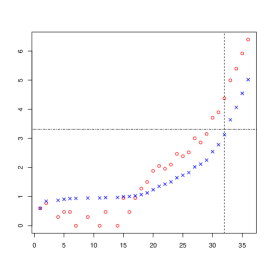
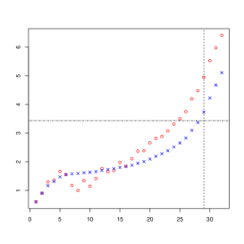
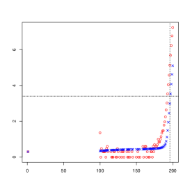
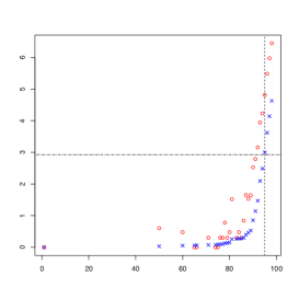
Figure 1: Sets of reads from left to right, top to bottom: SRR069579 (human), ERR000009 (yeast), SRR211279 (human), SRR959239 (human). The $x$-axis is the period and the $y$-axis is in $\log_{10}$ scale. The circles represent $n(x)$ and the crosses $\sum_{i=1}^{x}\frac{n(x)}{x}.$ The dash vertical line corresponds to the final $m\alpha$ (computed in the experimental results in Section 4) and the horizontal to $0.02\frac{n}{m}.$

3 Approximation algorithm

For two strings $u,v$ we define the overlap of $u$ and $v$, denoted $\textrm{ov}(u,v)$, as the longest suffix of $u$ that is also a prefix of $v$. Also, we define the prefix of $u$ relatively to $v$, denoted $\textrm{pref}(u,v)$, as the string $x$ such that $u=x\,\textrm{ov}(u,v)$, i.e., the prefix of $u$ that does not overlap $v$.

The prefix graph (also called the distance graph) of $S$ is a complete directed graph with the vertex set $S$ and the edges $(s_{i},s_{j})$ of weight equal to the length $|\textrm{pref}(s_{i},s_{j})|$.

We consider the classical algorithm of [2, 20], which gives a general framework. This algorithm is proved to be a 3 approximation algorithm in the general case. We prove below that applied on NGS data the approximation factor can be improved. The scheme of the algorithm is the following:

1. Compute a maximal cycle decomposition on the prefix graph

2. For each cycle $c_{i}$ choose one of the strings in $c_{i}$ as a representative string $r_{i}$.

3. $\sigma_{i}=(\textrm{pref}(r_{i},r_{i+1})\cdot...\cdot\textrm{pref}(r_{k},r_{i}))\cdot r_{i}$ (cycle from $r_{i}$ concatenated with $r_{i}$).

4. Let $S_{\sigma}=\{\sigma_{i}\}$ and $w_{\sigma}$ as a concatenation of all $\sigma_{i}$.

5. Compress $w_{\sigma}$ using an SSP compression algorithm.

The cycle decomposition produces cycles of several lengths. The period of a cycle is given by its length. We split the set of cycles, in two parts, the small cycles of period less than or equal to $m\alpha$, and the larger ones, denoted large. We now focus on the number of small cycles. The weight of a cycle is the sum of the weights of its edges and let $\mbox{wt}(\mathcal{C})$ be the sum of the weights of all cycles.

Lemma 1

Let $c\in\mathcal{C}$ be a cycle and $s$ a sequence in the cycle, then $\mbox{period}(c)\geq\mbox{period}(s)$

Proof. Each sequence in the cycle can be expressed by turning around the cycle. If $\mbox{period}(c)<\mbox{period}(s)$, then $\mbox{period}(c)$ is also a period of $s$, which is smaller than its smallest period, contradiction. $\Box$

Corollary 1

Let $c\in\mathcal{C}$ be a cycle and $s_{1}\ldots s_{k}$ the sequences in $\mathcal{C}$. Then $\mbox{period}(c)\geq\mbox{max}\{\mbox{period}(s_{i})\}.$

Proof. Directly derives from lemma 1. $\Box$

Lemma 2

Let $c\in\mathcal{C}$ be a cycle and $s_{1}\ldots s_{k}$ the sequences in $\mathcal{C}$. If $\mbox{period}(c)\leq m\alpha$, $\mbox{period}(s_{i})\leq m\alpha.$

Proof. By corollary 1, the periods of all sequences in a cycle are smaller than or equal to the period of the cycle. $\Box$

Corollary 2

Let $1\leq i\leq m$, the maximal number of cycles of period less or equal to $i$ is bounded by $\frac{1}{2}\sum_{k=1}^{i}n(i).$

Proof. A cycle contains at least two sequences. By Lemma 2, all the sequences in $c$ of period $i$ must have a period less than or equal to $i$ and there are only $\frac{1}{2}\sum_{k=1}^{i}n(i)$ such sequences. $\Box$

3.1 Analysis of the algorithm

We bounded the number of small cycles relatively to $\alpha$. Let us now take this into account while analysing the approximation algorithm. Obviously, $w_{\sigma}$ is a superstring of $S$. Let us bound its size.

Lemma 3

$$|w_{\sigma}|=\sum\left|\sigma_{i}\right|\leq\mbox{wt}(\mathcal{C})+\mbox{wt}(\mathcal{C})\frac{1}{\alpha}+\frac{\textrm{\it sp}\cdot m}{2}\leq(1+\frac{1}{\alpha})\mbox{\it OPT}+\frac{\textrm{\it sp}\cdot m}{2}$$

Proof. A $\sigma_{i}$ is formed on a cycle as $(\textrm{pref}(r_{i},r_{i+1})\cdot...\cdot\textrm{pref}(r_{k},r_{i}))\cdot r_{i}.$ We first sum over all the $\sigma_{i}$ the prefixes of each $\sigma_{i}$ corresponding to the cycle. This leads to a first global $\mbox{wt}(\mathcal{C}).$ Then we consider the sizes of the $r_{i}$ for the large cycles. The point is that all $r_{i}$ have the same length $m$, and that each $r_{i}$ can be represented (or expressed) by turning around the cycle it corresponds to (see Figure 2). As large cycles have a period of at least $m\alpha$, turning $\frac{1}{\alpha}\textrm{period}(c_{i})$ around the cycle $c_{i}$ is enough to read $r_{i}$. Thus, the sum over all large cycles of $[r_{i}|$ is bounded by $\mbox{\em wt}(\mathcal{C})\frac{1}{\alpha}.$

Figure 2: Expressing a representative $r$ over the cycle it belongs to. The period of cycle (a) is larger than $m\alpha$ and thus the expression of $r$ requires only $1/\alpha$ cycles. The period of cycle (b) is $2\leq i<m\alpha$ and the expression of $r$ thus requires $m/i$ cycles, which can be at maximum $m/2$

The remaining step is counting the sum of the $r_{i}$ corresponding to $n_{\alpha}$ small cycles.

As, by corollary 2, there are at most $\textrm{\it sp}/2$ such cycles, the sum of the corresponding $r_{i}$ is bounded by $\textrm{\it sp}\cdot m/2$. This would already be an acceptable bound since sp is small relatively to $m/n$. But this implies counting $m$ for all small cycles, independently of the periods of the cycles, which can vary from 2 to $m\alpha$. The larger the period of the cycle, the less we need to turn on the cycle to read the representative $r_{i}$. Thus our worst case for counting the small cycles from period $1$ to $m\alpha$ is when there is a maximum of smaller cycles at each step $2\leq k\leq m\alpha$ and, by corollary 2, this maximum from $k-1$ to $k$ can only be increased by $n(k)$. Expressing the representative of each such $n(k)$ additionnal cycles of period $k$, requires $n(k)\frac{m}{k}.$ Thus, the expression of the representatives of all the small cycles is bounded by $\frac{1}{2}\sum_{i=1}^{m\alpha}\frac{n(i)\cdot m}{i}=\frac{\textrm{\it sp}\cdot m}{2}.$

Eventually, as $\mbox{wt}(\mathcal{C})\leq\mbox{\it OPT}$, the result follows. $\Box$

We then compress $S_{\sigma}$ using the guaranteed compression algorithm of $\frac{38}{63}$ [12], similarly to the classical approaches related to the superstring approximation. We define $\mbox{OPT}_{\sigma}$ as an optimal minimal superstring on $S_{\sigma}$ and $\tau$ as the result of the compression algorithm on $S_{\sigma}.$ The next lemma [2, 20] allows us to link $\mbox{\it OPT}_{\sigma}$ and OPT.

Lemma 4

$\mbox{\it OPT}_{\sigma}<\mbox{\it OPT}+\mbox{wt}(\mathcal{C})$

By applying the compression algorithm on $S_{\sigma}$, we thus derive the following result:

Lemma 5

$|\tau|\leq 2\mbox{\it OPT}+\frac{38}{63}\left(\frac{1-\alpha}{\alpha}\right)\mbox{\it OPT}+\frac{38}{126}\textrm{\it sp}\cdot m$

Proof. Lemma 4 gives $\mbox{\it OPT}_{\sigma}<\mbox{\it OPT}+\mbox{wt}(\mathcal{C})\leq 2\mbox{\it OPT}$ (see Figure 3). The distance from $\mbox{\it OPT}_{\sigma}$ to $|w_{\sigma}|$ is greater than or equal to $|w_{\sigma}|-{2\mbox{\it OPT}}.$ In the worst case it is equal, then the compression algorithm applies a compression factor $38/63$ to this distance, which leads to the result.

Figure 3: Compressing $w_{\sigma}$ using the $38/63$ algorithm [12]

$\Box$

An important point is that $OPT\geq n$, since any superstring contains at least one base of each sequence. As $\textrm{\it sp}=\mbox{\em perc}_{\alpha}\frac{n}{m}$, $\frac{38}{63}\frac{\textrm{\it sp}m}{2}\leq\frac{38}{126}\mbox{\em perc}_{\alpha}\mbox{OPT}$

Theorem 1

$$|\tau|\leq 2\mbox{\it OPT}+\frac{38}{63}\left(\frac{1-\alpha}{\alpha}\right)\mbox{\it OPT}+\frac{38}{126}\mbox{\em perc}_{\alpha}\mbox{OPT}$$

period	nbseq	cum. nbseq	$\alpha$	$1+\frac{1}{\alpha}$	$2+\frac{38}{63}\left(\frac{1-\alpha}{\alpha}\right)$	$\frac{38}{126}\textrm{\it sp}\frac{m}{n}$	$\beta$
1	4	4	0.0277778	37	23.1111	1.74749e-05	23.1111
2	6	10	0.0555556	19	12.254	3.0581e-05	12.254
$\ldots$	$\ldots$	$\ldots$	$\ldots$	$\ldots$	$\ldots$	$\ldots$	$\ldots$
32	23746	41326	0.888889	2.125	2.0754	0.00588868	2.08129
33	98795	140121	0.916667	2.09091	2.05483	0.0189677	2.0738
34	247451	387572	0.944444	2.05882	2.03548	0.0507631	2.08624
35	829535	1217107	0.972222	2.02857	2.01723	0.154306	2.17154
36	2485202	3702309	1	2	2	0.455893	2.45589

Table 1: SRR069579 read set, 3702309 reads of size 36. $\beta=2+\frac{38}{63}\left(\frac{1-\alpha}{\alpha}\right)+\frac{38}{126}\textrm{\it sp}\frac{m}{n}$

period	nbseq	cum. nbseq	$\alpha$	$1+\frac{1}{\alpha}$	$2+\frac{38}{63}\left(\frac{1-\alpha}{\alpha}\right)$	$\frac{38}{126}\textrm{\it sp}\frac{m}{n}$	$\beta$
1	4	4	0.03125	33	20.6984	8.83862e-06	20.6984
2	8	12	0.0625	17	11.0476	1.76772e-05	11.0476
$\ldots$	$\ldots$	$\ldots$	$\ldots$	$\ldots$	$\ldots$	$\ldots$	$\ldots$
28	30474	61366	0.875	2.14286	2.08617	0.00518227	2.09135
29	89474	150840	0.90625	2.10345	2.0624	0.0119997	2.0744
30	341160	492000	0.9375	2.06667	2.04021	0.0371279	2.07734
31	953389	1445389	0.96875	2.03226	2.01946	0.105085	2.12454
32	2606944	4052333	1	2	2	0.285099	2.2851

Table 2: ERR000009 read set, 4052333 reads of size 32

period	nbseq	cum. nbseq	$\alpha$	$1+\frac{1}{\alpha}$	$2+\frac{38}{63}\left(\frac{1-\alpha}{\alpha}\right)$	$\frac{38}{126}\textrm{\it sp}\frac{m}{n}$	$\beta$
1	2	2	0.005	201	122.032	4.80545e-06	122.032
100	23	25	0.5	3	2.60317	5.35808e-06	2.60318
$\ldots$	$\ldots$	$\ldots$	$\ldots$	$\ldots$	$\ldots$	$\ldots$	$\ldots$
195	38013	54574	0.975	2.02564	2.01547	0.00067972	2.01615
196	134284	188858	0.98	2.02041	2.01231	0.00232588	2.01464
197	473686	662544	0.985	2.01523	2.00919	0.00810323	2.01729
198	1685038	2347582	0.99	2.0101	2.00609	0.0285511	2.03464
199	5811666	8159248	0.995	2.00503	2.00303	0.0987212	2.10175
200	16944518	25103766	1	2	2	0.302286	2.30229

Table 3: SRR211279 read set, 25103766 reads of size 200

period	nbseq	cum. nbseq	$\alpha$	$1+\frac{1}{\alpha}$	$2+\frac{38}{63}\left(\frac{1-\alpha}{\alpha}\right)$	$\frac{38}{126}\textrm{\it sp}\frac{m}{n}$	$\beta$
1	1	1	0.0102041	99	60.5079	7.13344e-06	60.5079
50	4	5	0.510204	2.96	2.57905	7.70411e-06	2.57906
$\ldots$	$\ldots$	$\ldots$	$\ldots$	$\ldots$	$\ldots$	$\ldots$	$\ldots$
94	17083	28491	0.959184	2.04255	2.02567	0.00218336	2.02785
95	65228	93719	0.969388	2.03158	2.01905	0.00708125	2.02613
96	302973	396692	0.979592	2.02083	2.01257	0.0295941	2.04216
97	942267	1338959	0.989796	2.01031	2.00622	0.098889	2.10511
98	2804284	4143243	1	2	2	0.303013	2.30301

Table 4: SRR959239 read set, 4143243 reads of size 98

4 Experimental results

We present experimental results for the sets of reads SRR069579 (Table 1), ERR000009 (Table 2), SRR211279 (Table 3), and SRR959239 (Table 4).

In each table, for each period $i$ from $1$ to $m$ we show : (a) $n(i)$, (b) the cumulative number of sequences, (c) the value of $\alpha$ corresponding to $i/m$, (d) the value of $1+\frac{1}{\alpha}$, (e) $2+\frac{38}{63}\left(\frac{1-\alpha}{\alpha}\right)$ which corresponds to the term of equation 1 due to the large cycles, (f) $\frac{38}{126}\textrm{\it sp}\frac{m}{n}$ which is the part of the final ratio brought by the small cycles, and eventually (g) $\beta=2+\frac{38}{63}\left(\frac{1-\alpha}{\alpha}\right)+\frac{38}{126}\textrm{\it sp}\frac{m}{n}$, the final ratio that can be reached by using the value of $\alpha$ from the previous line in the table.

The resulting approximation ratios on the read sets cited above are respectively 2.0738, 2.09, 2.01464 and 2.02623.

References

- [1] C. Armen and C. Stein. A superstring approximation algorithm. Discrete Applied Mathematics, 88(1–3):29 – 57, 1998. Computational Molecular Biology {DAM} - {CMB} Series.
- [2] A. Blum, T. Jiang, M. Li, J. Tromp, and M. Yannakakis. Linear approximation of shortest superstrings. J. ACM, 41(4):630–647, July 1994.
- [3] D. Breslauer, T. Jiang, and Z. Jiang. Rotations of periodic strings and short superstrings. Journal of Algorithms, 24(2):340 – 353, 1997.
- [4] A. Chris and S. Clifford. Algorithms and Data Structures: 4th International Workshop, WADS ’95 Kingston, Canada, August 16–18, 1995 Proceedings, chapter Improved length bounds for the shortest superstring problem, pages 494–505. Springer Berlin Heidelberg, Berlin, Heidelberg, 1995.
- [5] M. Crochemore, M. Cygan, C. S. Iliopoulos, M. Kubica, J. Radoszewski, W. Rytter, and T. Walen. Algorithms for three versions of the shortest common superstring problem. In CPM, volume 6129 of Lecture Notes in Computer Science, pages 299–309. Springer, 2010.
- [6] A. Czumaj, L. Gasieniec, M. Piotrów, and W. Rytter. Sequential and parallel approximation of shortest superstrings. Journal of Algorithms, 23(1):74 – 100, 1997.
- [7] G. Fici, T. Kociumaka, J. Radoszewski, W. Rytter, and T. Walen. On the greedy algorithm for the shortest common superstring problem with reversals. Inf. Process. Lett., 116(3):245–251, 2016.
- [8] J. Gallant, D. Maier, and J. Astorer. On finding minimal length superstrings. Journal of Computer and System Sciences, 20(1):50 – 58, 1980.
- [9] M. R. Garey and D. S. Johnson. Computers and Intractability; A Guide to the Theory of NP-Completeness. W. H. Freeman & Co., New York, NY, USA, 1990.
- [10] A. Golovnev, A. S. Kulikov, and I. Mihajlin. Approximating shortest superstring problem using de bruijn graphs. In CPM, volume 7922 of Lecture Notes in Computer Science, pages 120–129. Springer, 2013.
- [11] H. Kaplan and N. Shafrir. The greedy algorithm for shortest superstrings. Inf. Process. Lett., 93(1):13–17, 2005.
- [12] S. R. Kosaraju, J. K. Park, and C. Stein. Long tours and short superstrings. In Foundations of Computer Science, 1994 Proceedings., 35th Annual Symposium on, pages 166–177, Nov 1994.
- [13] M. Li. Towards a DNA sequencing theory (learning a string). In Proc. of the 31st Symposium on the Foundations of Comp. Sci., pages 125–134. IEEE Computer Society Press, Los Alamitos, CA, 1990.
- [14] M. Mucha. Lyndon words and short superstrings. In SODA, pages 958–972. SIAM, 2013.
- [15] Sascha Ott. Graph-Theoretic Concepts in Computer Science: 25th International Workshop, WG’99 Ascona, Switzerland, June 17–19, 1999 Proceedings, chapter Lower Bounds for Approximating Shortest Superstrings over an Alphabet of Size 2, pages 55–64. Springer Berlin Heidelberg, Berlin, Heidelberg, 1999.
- [16] K. E. Paluch, K. M. Elbassioni, and A. van Zuylen. Simpler approximation of the maximum asymmetric traveling salesman problem. In STACS, volume 14 of LIPIcs, pages 501–506. Schloss Dagstuhl - Leibniz-Zentrum fuer Informatik, 2012.
- [17] Z. Sweedyk. a -approximation algorithm for shortest superstring. SIAM J. Comput., 29(3):954–986, December 1999.
- [18] J. Tarhio and E. Ukkonen. A greedy approximation algorithm for constructing shortest common superstrings. Theoretical Computer Science, 57(1):131 – 145, 1988.
- [19] S.-H. Teng and F. F. Yao. Approximating shortest superstrings. SIAM J. Comput., 26(2):410–417, 1997.
- [20] V. V. Vazirani. Approximation Algorithms. Springer-Verlag New York, Inc., New York, NY, USA, 2001.
- [21] Y. W. Yu. Approximation hardness of shortest common superstring variants. CoRR, abs/1602.08648, 2016.