The Flavoured BFSS Model at High Temperature

Abstract

We study the high-temperature series expansion of the Berkooz-Douglas matrix model, which describes the D0/D4–brane system. At high temperature the model is weakly coupled and we develop the series to second order. We check our results against the high-temperature regime of the bosonic model (without fermions) and find excellent agreement. We track the temperature dependence of the bosonic model and find backreaction of the fundamental fields lifts the zero-temperature adjoint mass degeneracy. In the low-temperature phase the system is well described by a gaussian model with three masses $m^{t}_{A}=1.964\pm 0.003$, $m^{l}_{A}=2.001\pm 0.003$ and $m_{f}=1.463\pm 0.001$, the adjoint longitudinal and transverse masses and the mass of the fundamental fields respectively.

1 Introduction

The Berkooz-Douglas model (BD model) Berkooz:1996is was introduced as a non-perturbative formulation of M-theory in the presence of a background of longitudinal M5-branes with the M2-brane quantised in light-cone gauge. Its action is written as that of the BFSS model Banks:1996vh with additional fundamental hypermultiplets to describe the M5-branes. The BFSS model can also be viewed as a many-body system of D0-branes of the IIA superstring. In this framework the BD model is a D0/D4 system with the massless case being the D0/D4 intersection. When the number of D0-branes far exceeds that of the D4-branes the dynamics of the D0-branes is only weakly affected by that of the D4-branes and is captured by the IIA supergravity background holographically dual to the BFSS model. In this context the D4-branes, representing the fundamental fields of the BD model, are treated as Born-Infeld probe 4-branes. This holographic set up is a tractable realisation of gauge/gravity duality with flavour.

Both the BFSS model and the BD model are supersymmetric quantum mechanical models with an $SU(N)$ gauge symmetry. When they are put in a thermal bath they become strongly coupled at low temperature. At finite temperature their gravity duals involve a black hole whose Hawking-temperature is that of the thermal bath. These duals can be used to provide non-perturbative predictions at low temperature. The BFSS and BD models can also be studied by the standard non-perturbative field theory method of Monte Carlo simulation. These models therefore provide excellent candidates for testing gauge/gravity duality non-perturbatively and in a broken supersymmetric setting.

There are now several non-perturbative studies of the BFSS model Anagnostopoulos:2007fw ; Catterall:2008yz ; Kadoh:2015mka ; Filev:2015hia ; Hanada:2016zxj and several recent reviewsJoseph:2015xwa ; Hanada:2016jok ; O'Connor:2016goh . Also, the BD model was recently studied non-perturbatively in Filev:2015cmz . In all cases the predictions from the gauge/gravity duals were found to be in excellent agreement with that of Monte Carlo simulations of the finite-temperature models.

The situation is conceptually simpler at high temperature as the dimensionless inverse temperature, scaled in terms of the BD-coupling, provides a natural small parameter for the model. In this paper, we obtain the first two terms in the high-temperature expansion of the BD model.

In the high-temperature limit only the bosonic Matsubara zero modes survive and the resulting model is a pure potential. This potential, which provides the non-perturbative aspect of our high-temperature study, also plays a role in the ADHM construction Tong:2005un . We study the model for adjoint matrix size $N$ between $4$ and $32$ for $N_{f}=1$ (with $N_{f}$ the number of D4-branes) and for $N_{f}$ between $2$ and $16$ for $N$ from $9$ to $20$. For $N_{f}\geq 2N$ we find that the system has difficulties with ergodicity. In particular, for $N_{f}=2N$ and $N_{f}=2N+1$ the system failed to thermalise satisfactorily. In contrast the system has no difficulties for $N_{f}=2N-1$. This condition is closely related to the singularity structure of instanton moduli space, where irreducible $SU(N_{f})$ instantons of Chern number $N$ exist only for $N\geq\frac{N_{f}}{2}$ Atiyah:1978wi ; Nash:1991pb . The moduli space of such instantons is equivalent to the zero locus of the potential with $X^{a}=0$ and ${\cal D}^{A}=0$ (see equation (4)). This moduli space is in general singular and non-singular only when this bound is satisfied.

There is also a natural $1+1$ dimensional analogue of the BD model, which has ${\cal N}=4$ supersymmetry, associated with the D1/D5 system of VanRaamsdonk:2001cg , whose BFSS relative was discussed in Aharony:2004ig ; Kawahara:2007fn ; Mandal:2009vz . When the Euclidean finite-temperature version of this $1+1$ dimensional quantum field theory is considered on a torus with the spatial circle of period $\beta$ and euclidean time of period $1/T$, then at high temperature the fermions decouple and one is left with the purely bosonic version of the BD model. We refer to this model as the bosonic BD model and study the small period behaviour (equivalent for us to our high-temperature regime) of the massless version of this model as a check on our high-temperature series. We find the high-temperature series results are in excellent agreement with Monte Carlo simulations of the bosonic BD model. By fitting the dependence, of the expectation values of our observables, on the number of flavour multiplets, $N_{f}$, we find that extrapolation, to $N_{f}=0$, agrees well with the corresponding observables of the BFSS model.

As $\beta$, the inverse temperature, grows the bosonic BD model undergoes a set of phase transitions. These are the phase transitions of the bosonic BFSS model. We find the high-temperature series expansion is valid up to $\beta\sim 1/2$, which is just below the phase transition region. Above the transition the bosonic BD model is well described by free massive fields, where the backreaction of the fundamental fields has lifted the degeneracy of the longitudinal and transverse masses.

The principal results of this paper are:

• We obtain expansions for observables of the BD model to second order in a high-temperature series.

• We tabulate the coefficients of this expansion as functions of $N$ and $N_{f}$ in the range $4\leq N\leq 32$ and $1\leq N_{f}\leq 16$.

• We measure the expectation values of the composite operator $\langle r^{2}\rangle_{\text{bos}}$, (see equation (8)), and the mass susceptibility $\langle{\mathcal{C}}^{m}\rangle_{\text{bos}}$, (see equation (62)), of the bosonic BD model as a function of temperature down to zero and use it to check our coefficients for the high-temperature series of the full BD model.

• We find that the fundamental fields of the bosonic BD model have mass $m_{f}=1.463\pm 0.001$.

• We measure the backreacted mass of the longitudinal adjoint scalars to be $m^{l}_{A}=2.001\pm 0.003$ and find that the transverse mass is largely unaffected by backreaction being $m^{t}_{A}=1.964\pm 0.003$, which should be compared with the bosonic BFSS model, where the fields have mass $m_{A}=1.965\pm 0.007$.

• We use the measured masses to predict the zero-temperature values of our fundamental field observables $\langle r^{2}\rangle_{\text{bos}}$ and mass susceptibility $\langle{\mathcal{C}}^{m}\rangle_{\text{bos}}$ and find excellent agreement with direct measurements.

The paper is organised as follows: In section 2 we present the finite-temperature BD model and describe our notation and observables. In section 3 we set up and implement the high-temperature series expansion working to second order in the inverse temperature $\beta$. Section 4 describes the dependence of our observables on the coefficients in the expansion, which must be determined by numerical simulation of the zero-mode model. In Section 5 we perform lattice simulations of the bosonic BD model and find excellent agreement with the high-temperature expansion. We also find the low-temperature phase of the model is well described by a system of gaussian quantum fields. Section 6 gives our concluding remarks. There are two appendices; appendix A gives tables, for different $N$ and $N_{f}$, of the coefficients determined non-perturbatively while appendix B presents graphs of predictions for the high-temperature behaviour of our observables for the supersymmetric model.

2 The Berkooz-Douglas Model

We begin by describing the field content of the model following the notation used in (VanRaamsdonk:2001cg, ). The action of the BFSS model is given by

$$S_{\rm BFSS}=\frac{1}{g^{2}}\int dt\sum_{i=1}^{9}\,{\rm Tr}\left\{\frac{1}{2}({\cal D}_{0}X^{i})^{2}+\frac{1}{4}[X^{i},X^{j}]^{2}-\frac{i}{2}\Psi^{T}C_{10}\,\Gamma^{0}{\cal D}_{0}\Psi+\frac{1}{2}\Psi^{T}C_{10}\,\Gamma^{i}[X^{i},\Psi]\right\}\ ,$$ (1)

where ${\cal D}_{0}\;\cdot=\partial_{t}\;\cdot-i[A,\;\cdot\;]$, $\Psi$ is a thirty-two component Majorana–Weyl spinor, $\Gamma^{\mu}$ are ten dimensional gamma matrices and $C_{10}$ is the charge conjugation matrix satisfying $C_{10}\Gamma^{\mu}C_{10}^{-1}=-{\Gamma^{\mu}}^{T}$. The fields $X^{i}$ and $\Psi$ are in the adjoint representation of the gauge symmetry group $SU(N)$ and $A$ is the gauge field.

To describe the addition of the fundamental fields we break the $SO(9)$ vector $X^{i}$ into an $SO(5)$ vector $X^{a}$ and an $SO(4)$ vector which we re-express as $X_{\rho\dot{\rho}}$ via

$$X_{\rho\dot{\rho}}=\frac{i}{\sqrt{2}}\sum_{m=1}^{4}\sigma^{m}_{\;\;\rho\dot{\rho}}X^{10-m},$$ (2)

where $\sigma^{4}=-i\mathbf{1}_{2}$ and $\sigma^{A}$’s ($A=1,2,3$) are the Pauli matrices. The $X_{\rho\dot{\rho}}$ ($\rho,\dot{\rho}=1,2$) are complex scalars which together transform as a real vector of $SO(4)$ which satisfies the reality condition $X_{\rho\dot{\rho}}=\varepsilon_{\rho\sigma}\varepsilon_{\dot{\rho}\dot{\sigma}}\bar{X}^{\sigma\dot{\sigma}}$. The indices $\rho$ and $\dot{\rho}$ are those of $SU(2)_{R}$ and $SU(2)_{L}$, respectively, where $SO(4)=SU(2)_{L}\times SU(2)_{R}$.

The nine BFSS scalar fields, $X^{i}$, become $X^{a}$ ($a=1,\cdots,5$) and $X_{\rho\dot{\rho}}$. The sixteen adjoint fermions of the BFSS model become $\lambda_{\rho}$ and $\theta_{\dot{\rho}}$ with $\lambda_{\rho}$ being $SO(5,1)$ symplectic Majorana-Weyl spinors of positive chirality and satisfying $\lambda_{\rho}=\varepsilon_{\rho\sigma}(\lambda^{c})^{\sigma}$ while $\theta_{\dot{\rho}}$ are symplectic Majorana-Weyl spinors of negative chirality satisfying $\theta_{\dot{\rho}}=-\varepsilon_{\dot{\rho}\dot{\sigma}}(\theta^{c})^{\dot{\sigma}}$. They combine together to form an $SO(9,1)$ Majorana-Weyl spinor in the adjoint of $SU(N)$. This $SO(9)$ symmetry is recovered only if the fundamental fields are turned off.

To describe the longitudinal M5-branes (or D4-branes), we have $\Phi_{\rho}$ and $\chi$, which transform in the fundamental representations of both $SU(N)$ and the global $SU(N_{f})$ flavour symmetry. $\Phi_{\rho}$ are complex scalar fields with hermitian conjugates $\bar{\Phi}^{\rho}$, and $\chi$ is an $SO(5,1)$ spinor of negative chirality.

After rotating to imaginary time the Euclidean action describing the model at finite temperature $T=\beta^{-1}$ becomes:

$$S=N\int_{0}^{\beta}d\tau\, \Bigg{[}\operatorname{Tr}\left(\frac{1}{2}D_{\tau}X^{a}D_{\tau}X^{a}+\frac{1}{2}D_{\tau}\bar{X}^{\rho\dot{\rho}}D_{\tau}X_{\rho\dot{\rho}}+\frac{1}{2}\lambda^{\dagger\rho}D_{\tau}\lambda_{\rho}+\frac{1}{2}\theta^{\dagger\dot{\rho}}D_{\tau}\theta_{\dot{\rho}}\right)$$

$$+\operatorname{tr}\left(D_{\tau}\bar{\Phi}^{\rho}D_{\tau}\Phi_{\rho}+\chi^{\dagger}D_{\tau}\chi\right)$$

$$-\operatorname{Tr}\left(\frac{1}{4}[X^{a},X^{b}]^{2}+\frac{1}{2}[X^{a},\bar{X}^{\rho\dot{\rho}}][X^{a},X_{\rho\dot{\rho}}]\right)$$

$$+\frac{1}{2}\operatorname{Tr}\sum_{A=1}^{3}\mathcal{D}^{A}\mathcal{D}^{A}+\operatorname{tr}\left(\bar{\Phi}^{\rho}(X^{a}-m^{a})^{2}\Phi_{\rho}\right)$$

$$-\operatorname{Tr}\left(-\frac{1}{2}\lambda^{\dagger\rho}\gamma^{a}[X^{a},\lambda_{\rho}]+\frac{1}{2}\theta^{\dagger\dot{\rho}}\gamma^{a}[X^{a},\theta_{\dot{\rho}}]-\sqrt{2}i\varepsilon^{\rho\sigma}\theta^{\dagger\dot{\rho}}[X_{\sigma\dot{\rho}},\lambda_{\rho}]\right)$$

$$-\operatorname{tr}\left(\chi^{\dagger}\gamma^{a}(X^{a}-m^{a})\chi+\sqrt{2}i\varepsilon^{\rho\sigma}\chi^{\dagger}\lambda_{\rho}\Phi_{\sigma}+\sqrt{2}i\varepsilon_{\rho\sigma}\bar{\Phi}^{\rho}\lambda^{\dagger\sigma}\chi\right)\,\Bigg{]},$$ (3)

where

$$\mathcal{D}^{A}=\sigma^{A\;\sigma}_{\rho}\left(\frac{1}{2}[\bar{X}^{\rho\dot{\rho}},X_{\sigma\dot{\rho}}]-\Phi_{\sigma}\bar{\Phi}^{\rho}\right)\,,$$ (4)

with $D_{\tau}$ the covariant derivative which, for the fields of the fundamental multiplet, $\Phi_{\rho}$ and $\chi$, acts as $D_{\tau}\;\cdot=(\partial_{\tau}-iA)\;\cdot$ . The trace of $SU(N)$ is written as $\operatorname{Tr}$ while that of $SU(N_{f})$ is denoted by $\operatorname{tr}$. The diagonal matrices, $m^{a}$, correspond to the transverse positions of the D4-branes.

We fix the static gauge: $\partial_{\tau}A=0$, so the path integral requires the corresponding ghost fields $c$ and $\bar{c}$ with the ghost term $N\int_{0}^{\beta}d\tau\,\operatorname{Tr}\partial_{\tau}\bar{c}D_{\tau}c$ added to the action (3).

We will restrict our attention to $m^{a}=0$ so that the D4-branes are attached to the D0-branes, and the strings between D0 and D4 are massless, i.e. the fundamental fields are massless. The factor of $N$ in front of the integral in (3) is the remnant of the ’t Hooft coupling $\lambda=g^{2}N$ which is kept fixed and absorbed into $\tau$ and the fields with $\beta=\lambda^{1/3}/T$. Note that without loss of generality we can set $\lambda=1$.

As discussed in the introduction, the BFSS model is the matrix regularization of a supermembrane theory deWit:1988ig , so the BFSS part of this model can be also interpreted as M2-brane dynamics. In this context the D4-branes lift to M5-branes and the model can describe M2-branes ending on longitudinal M5-branes.

The BD model is a version of supersymmetric quantum mechanics and could in principle be treated by Hamiltonian methods. The partition function is then

$$Z=Tr({\rm e}^{-\beta H})=\int[dX][d\lambda][d\theta][d\Phi][d\bar{\Phi}][d\chi][d\chi^{\dagger}][dA]{\rm e}^{-S}$$ (5)

with $Tr$ the trace over the Hilbert space of the Hamiltonian restricted to its gauge invariant subspace and the action $S$, in the path integral, is given by equation (3).

The measure in the path integral for the partition function (5) has a hidden dependence on temperature due to the presence of the Van Vleck-Morette determinant DeWitt:1992cy in the definition of the path integral measure. This determinant arises from the kinetic contribution to the action (3) which, as written, is temperature dependent. To remove the temperature dependence from the measure, we rescale the variables in the original action (3) so that the kinetic terms, including the gauge potential, are independent of $\beta$. For this $\tau\rightarrow\beta\tau$, $X^{i}\rightarrow\beta^{\frac{1}{2}}X^{i}$, $\Phi_{\rho}\rightarrow\beta^{\frac{1}{2}}\Phi_{\rho}$, $A\rightarrow\beta^{-1}A$, $c\rightarrow\beta^{\frac{1}{2}}c$ and ${\bar{c}}\rightarrow\beta^{\frac{1}{2}}{\bar{c}}$. The fermions do not need rescaling. The path integral measure is now temperature independent and, when the mass is zero, the only temperature dependence is $\beta^{3}$ for the bosonic potential and $\beta^{3/2}$ for the fermionic potential. If the mass term is included it enters as $\frac{\beta m^{a}}{\beta^{\frac{3}{2}}}$ in the potential with the overall scales of $\beta^{3}$ and $\beta^{3/2}$ in the bosonic and fermionic contributions respectively. The temperature dependence of the model is now explicit.

The principal observable of the model is the energy, $E=\langle H\rangle/N^{2}$. Once the temperature dependence of the model has been made explicit, as described above, one can then simply note that $N^{2}E$ is minus the derivative of logarithm of the partition function with respect to $\beta$, returning to the original variables one readily sees that in the path integral formulation:

$$E =\langle\varepsilon_{b}\rangle+\langle\varepsilon_{f}\rangle\,,\quad\hbox{where}$$

$$\varepsilon_{b} =\frac{3}{N\beta}\int_{0}^{\beta}d\tau\bigg{[}\operatorname{Tr}\left(-\frac{1}{4}[X^{i},X^{j}]^{2}\right)$$

$$\hskip 71.13188pt+\operatorname{tr}\left(\bar{\Phi}^{\rho}X^{a\,2}\Phi_{\rho}-\bar{\Phi}^{\rho}[\bar{X}^{\sigma\dot{\rho}},X_{\rho\dot{\rho}}]\Phi_{\sigma}-\frac{1}{2}\bar{\Phi}^{\rho}\Phi_{\sigma}\bar{\Phi}^{\sigma}\Phi_{\rho}+\bar{\Phi}^{\rho}\Phi_{\rho}\bar{\Phi}^{\sigma}\Phi_{\sigma}\right)\bigg{]}\,,$$

$$\varepsilon_{f} =\frac{3}{2N\beta}\int_{0}^{\beta}d\tau\bigg{[}\operatorname{Tr}\left(\frac{1}{2}\lambda^{\dagger\rho}\gamma^{a}[X^{a},\lambda_{\rho}]-\frac{1}{2}\theta^{\dagger\dot{\rho}}\gamma^{a}[X^{a},\theta_{\dot{\rho}}]+\sqrt{2}i\varepsilon^{\rho\sigma}\theta^{\dagger\dot{\rho}}[X_{\sigma\dot{\rho}},\lambda_{\rho}]\right)$$

$$\hskip 71.13188pt+\operatorname{tr}\left(-\chi^{\dagger}\gamma^{a}X^{a}\chi-\sqrt{2}i\varepsilon^{\rho\sigma}\chi^{\dagger}\lambda_{\rho}\Phi_{\sigma}-\sqrt{2}i\varepsilon_{\rho\sigma}\bar{\Phi}^{\rho}\lambda^{\dagger\sigma}\chi\right)\bigg{]}\,.$$ (6)

We see only the potential contributes and the coefficients $3$ and $3/2$ of the bosonic and fermionic terms arise from the differentiation.

As in Kawahara:2007ib , there are two other interesting observables:

$$R^{2}=\frac{1}{N\beta}\int_{0}^{\beta}d\tau\operatorname{Tr}X^{i\;2}\,,\qquad P=\frac{1}{N}\operatorname{Tr}\left(\exp\left[i\beta A\right]\right)\,.$$ (7)

Here $R^{2}$ is a hermitian operator whose expectation value is a measure of the extent of the eigenvalue distribution of the scalars $X^{i}$ and $P$ is the Polyakov loop. Note: Path-ordering is not needed here for the Polyakov loop as we consider $A$ in the static gauge.

Since the model has new degrees of freedom it is important to consider other observables that capture properties of these new fields. The natural candidates are

$$r^{2}=\frac{1}{\beta N_{f}}\int_{0}^{\beta}d\tau\,\operatorname{tr}\bar{\Phi}^{\rho}\Phi_{\rho}\,,$$ (8)

which is the analogue of $R^{2}$ for the fundamental degrees of freedom, and the condensate defined as

$$c^{a}(m) =\frac{\partial}{\partial m^{a}}\left(-\frac{1}{N\beta}\log Z\right)=\left\langle\frac{1}{\beta}\int_{0}^{\beta}d\tau\operatorname{tr}\left\{2\bar{\Phi}^{\rho}(m^{a}-X^{a})\Phi_{\rho}+\chi^{\dagger}\gamma^{a}\chi\right\}\right\rangle.$$ (9)

However, for us, with $m^{a}=0$, $c^{a}$ will be zero. So our focus will be on the mass susceptibility

$$\langle{\mathcal{C}}^{m}\rangle:=\frac{\partial c^{a}}{\partial m^{a}}(0)\,,$$ (10)

i.e. the derivative with respect to $m^{a}$ with $a$ fixed (not summed over) and evaluated at $m^{a}=0$ where

$${\mathcal{C}}^{m} =\frac{2}{\beta}\int_{0}^{\beta}d\tau\operatorname{tr}\bar{\Phi}^{\rho}\Phi_{\rho}-\frac{N}{5\beta}\left(\int_{0}^{\beta}d\tau\operatorname{tr}\left\{-2\bar{\Phi}^{\rho}X^{a}\Phi_{\rho}+\chi^{\dagger}\gamma^{a}\chi\right\}\right)^{2}\,.$$ (11)

Here $a$ in (11) is summed over $a=1,\cdots,5$ and the same applies hereinafter.

3 High-Temperature Expansion

In this section, we develop the high-temperature expansion of the BD model. For very high temperatures only the Matsubara zero modes, i.e. the zero modes in a Fourier expansion, survive and the model reduces to a bosonic matrix model for these modes. A high-temperature series expansion is therefore obtained by developing a perturbative expansion of the model in the non-zero modes. The zero-modes must then be treated non-perturbatively and this is done by Monte Carlo simulation.

Our strategy is therefore to expand the model in Matsubara modes, show that the temperature can be seen as a coupling constant for these modes and then integrate out the non-zero modes order by order in perturbation theory to obtain an effective action for the zero modes, which can then be treated non-perturbatively.

To obtain the series to second order we will only need one loop computations. The non-zero mode integration can be done analytically and yields an effective action and observables in terms of the zero temperature variables. As a final step the integration over these zero modes must then be performed non-perturbatively via Monte Carlo simulation.

The Fourier expansion of the fields is given by

$$X^{i}(\tau)=\sum_{n\in\mathbb{Z}}X^{i}_{n}e^{2\pi in\tau/\beta},\quad\lambda_{\rho}(\tau)=\sum_{r\in\mathbb{Z}+\frac{1}{2}}\lambda_{r\rho}e^{2\pi ir\tau/\beta},\quad\theta_{\dot{\rho}}(\tau)=\sum_{r\in\mathbb{Z}+\frac{1}{2}}\theta_{r\dot{\rho}}e^{2\pi ir\tau/\beta},$$

$$c(\tau)=\sum_{n\in\mathbb{Z},n\neq 0}c_{n}e^{2\pi in\tau/\beta},\quad\bar{c}(\tau)=\sum_{n\in\mathbb{Z},n\neq 0}\bar{c}_{n}e^{-2\pi in\tau/\beta},$$

$$\Phi_{\rho}(\tau)=\sum_{n\in\mathbb{Z}}\Phi_{n\rho}e^{2\pi in\tau/\beta},\quad\chi(\tau)=\sum_{r\in\mathbb{Z}+\frac{1}{2}}\chi_{r}e^{2\pi ir\tau/\beta},$$ (12)

where thermal boundary conditions require that the bosons and ghosts are periodic in $\tau$ while the fermions are anti-periodic.

The action (3) now takes the form of the sum of a zero mode action, the kinetic term for the non-zero modes and an interaction term. As discussed above, in the high-temperature limit, only the zero-modes play a role. As the temperature is lowered one can integrate out the non-zero modes perturbatively with $\beta$ playing the role of a perturbation parameter. Using this procedure, the first two terms in the high-temperature expansion of $E$, $\langle R^{2}\rangle$ and $\langle P\rangle$ for the BFSS model were obtained in (Kawahara:2007ib, ). We follow the same method here and obtain the corresponding expansion of these observables for the BD model and for them the novel feature will be the additional dependence on $N_{f}$, the number of flavour multiplets. In addition we have the new observable $\langle r^{2}\rangle$ and $\langle{\mathcal{C}}^{m}\rangle$.

In order to develop the high-temperature series it is convenient to rescale the scalar fields in (3) as follows

$$X_{0}^{i}\rightarrow\beta^{-\frac{1}{4}}X_{0}^{i}\,,\qquad A\rightarrow\beta^{-\frac{1}{4}}A\,,\qquad\Phi_{0}\rightarrow\beta^{-\frac{1}{4}}\Phi_{0}\,,\qquad$$

$$X_{n\neq 0}^{i}\rightarrow\beta^{\frac{1}{2}}X_{n\neq 0}^{i}\,,\qquad\Phi_{n\neq 0}\rightarrow\beta^{\frac{1}{2}}\Phi_{n\neq 0}\,,\qquad c_{n}\rightarrow\beta^{\frac{1}{2}}c_{n}\,,\qquad\bar{c}_{n}\rightarrow\beta^{\frac{1}{2}}\bar{c}_{n}\,,$$ (13)

while the fermions remain unchanged. This rescaling makes the coefficients of the zero-mode terms and the kinetic terms independent of $\beta$ so that one can concentrate on the $\beta$-dependence, which now appears only in the interaction terms.

The rescaling (13) can be understood as the rescaling of section 2, which was necessary to remove the temperature dependence of the measure, followed by the further zero-mode rescaling $X_{0}^{i}\rightarrow\beta^{-\frac{3}{4}}X_{0}^{i}$, $\Phi_{0\rho}\rightarrow\beta^{-\frac{3}{4}}\Phi_{0\rho}$ and $A\rightarrow\beta^{\frac{3}{4}}A$. This zero-mode rescaling means the partition function becomes

$$Z=\beta^{-\frac{3}{4}(8(N^{2}-1)+4NN_{f})}\bar{Z}\,,$$ (14)

where ${\bar{Z}}$ is the partition function in terms of the rescaled fields of (13) and the only remaining temperature dependence is in $S_{\text{int}}$. We can now develop the high-temperature series by diagrammatic techniques with $\beta$ playing the role of a coupling.

The action is then written in terms of the variables of (13), which we will use for the remainder of the paper, as

$$S=S_{0}+S_{\text{kin}}+S_{\text{int}}\;,$$ (15)

where $S_{0}$ is a zero-mode action

$$S_{0} =-\frac{N}{4}\operatorname{Tr}\left([X_{0}^{i},X_{0}^{j}]^{2}+2[A,X_{0}^{i}]^{2}\right)+N\operatorname{tr}\bigg{(}\bar{\Phi}_{0}^{\rho}A^{2}\Phi_{0\rho}+\bar{\Phi}_{0}^{\rho}(X^{a}_{0})^{2}\Phi_{0\rho}$$

$$\hskip 113.81102pt-\bar{\Phi}_{0}^{\rho}[\bar{X}_{0}^{\sigma\dot{\rho}},X_{0\rho\dot{\rho}}]\Phi_{0\sigma}-\frac{1}{2}\bar{\Phi}_{0}^{\rho}\Phi_{0\sigma}\bar{\Phi}_{0}^{\sigma}\Phi_{0\rho}+\bar{\Phi}_{0}^{\rho}\Phi_{0\rho}\bar{\Phi}_{0}^{\sigma}\Phi_{0\sigma}\bigg{)},$$ (16)

$S_{\text{kin}}$ is the kinetic part of the action for non-zero modes

$$S_{\text{kin}}=\sum_{n\neq 0} \frac{(2\pi n)^{2}N}{2}\bigg{[}\operatorname{Tr}\left(X_{-n}^{a}X_{n}^{a}+\bar{X}^{\rho\dot{\rho}}_{-n}X_{n\rho\dot{\rho}}+2\bar{c}_{-n}c_{n}\right)+\operatorname{tr}\left(2\bar{\Phi}_{-n}^{\rho}\Phi_{n\rho}\right)\bigg{]}$$

$$+\sum_{r}\frac{2\pi irN}{2}\left[\operatorname{Tr}\left(\lambda_{-r}^{\dagger\rho}\lambda_{r\rho}+\theta_{-r}^{\dagger\dot{\rho}}\theta_{r\dot{\rho}}\right)+\operatorname{tr}\left(2\chi_{-r}^{\dagger}\chi_{r}\right)\right],$$ (17)

and $S_{\text{int}}$ is the interaction part of the action. The terms quadratic in non-zero modes present in $S_{\text{int}}$ but not present in the BFSS model are

$$\mathit{\Delta}S_{\text{int}} =-N\beta^{\frac{3}{4}}(V_{1}^{(A)}+V_{1}^{(B)})-N\beta^{\frac{3}{2}}(V_{2}^{(A)}+V_{2}^{(B)}+V_{3})+O(\beta^{\frac{9}{4}}),$$ (18)

where

$$V_{1}^{(A)}=4\pi\sum_{n\neq 0}n\operatorname{tr}(\bar{\Phi}^{\rho}_{-n}A\Phi_{n\rho})+\sum_{r}\operatorname{tr}(i\chi_{-r}^{\dagger}A\chi_{r}),$$

$$V_{1}^{(B)}=\sum_{r}\operatorname{tr}(\chi_{-r}^{\dagger}\gamma^{a}X_{0}^{a}\chi_{r}+\sqrt{2}i\varepsilon^{\rho\sigma}\chi_{-r}^{\dagger}\lambda_{r\rho}\Phi_{0\sigma}+\sqrt{2}i\varepsilon_{\rho\sigma}\bar{\Phi}_{0}^{\rho}\lambda^{\dagger\sigma}_{-r}\chi_{r}),$$

$$V_{2}^{(A)}=-\sum_{n\neq 0}\operatorname{tr}(\bar{\Phi}^{\rho}_{-n}A^{2}\Phi_{n\rho}),$$

$$V_{2}^{(B)}=-\sum_{n\neq 0}\operatorname{tr}\big{(}\bar{\Phi}^{\rho}_{-n}X_{0}^{a\;2}\Phi_{n\rho}+\bar{\Phi}^{\rho}_{0}X^{a}_{-n}X^{a}_{n}\Phi_{0\rho}-\bar{\Phi}_{-n}^{\rho}[\bar{X}_{0}^{\sigma\dot{\rho}},X_{0\rho\dot{\rho}}]\Phi_{n\sigma}-\bar{\Phi}_{0}^{\rho}[\bar{X}_{-n}^{\sigma\dot{\rho}},X_{n\rho\dot{\rho}}]\Phi_{0\sigma}$$

$$\hskip 79.66771pt-\bar{\Phi}_{-n}^{\rho}\Phi_{0\sigma}\bar{\Phi}_{0}^{\sigma}\Phi_{n\rho}-\bar{\Phi}_{-n}^{\rho}\Phi_{n\sigma}\bar{\Phi}_{0}^{\sigma}\Phi_{0\rho}+2\bar{\Phi}_{-n}^{\rho}\Phi_{0\rho}\bar{\Phi}_{0}^{\sigma}\Phi_{n\sigma}+2\bar{\Phi}_{-n}^{\rho}\Phi_{n\rho}\bar{\Phi}_{0}^{\sigma}\Phi_{0\sigma}\big{)},$$

$$V_{3}=-\sum_{n\neq 0}\operatorname{tr}\Big{[}(\bar{\Phi}^{\rho}_{-n}X^{a}_{n}X^{a}_{0}\Phi_{0\rho}+\bar{\Phi}^{\rho}_{-n}X^{a}_{0}X^{a}_{n}\Phi_{0\rho}+\bar{\Phi}^{\rho}_{0}X^{a}_{-n}X^{a}_{0}\Phi_{n\rho}+\bar{\Phi}^{\rho}_{0}X^{a}_{0}X^{a}_{-n}\Phi_{n\rho})$$

$$\hskip 56.9055pt-(\bar{\Phi}_{-n}^{\rho}[\bar{X}_{n}^{\sigma\dot{\rho}},X_{0\rho\dot{\rho}}]\Phi_{0\sigma}+\bar{\Phi}_{-n}^{\rho}[\bar{X}_{0}^{\sigma\dot{\rho}},X_{n\rho\dot{\rho}}]\Phi_{0\sigma}$$

$$\hskip 71.13188pt+\bar{\Phi}_{0}^{\rho}[\bar{X}_{-n}^{\sigma\dot{\rho}},X_{0\rho\dot{\rho}}]\Phi_{n\sigma}+\bar{\Phi}_{0}^{\rho}[\bar{X}_{0}^{\sigma\dot{\rho}},X_{-n\rho\dot{\rho}}]\Phi_{n\sigma})$$

$$\hskip 56.9055pt-\frac{1}{2}(\bar{\Phi}_{-n}^{\rho}\Phi_{0\sigma}\bar{\Phi}_{n}^{\sigma}\Phi_{0\rho}+\bar{\Phi}_{0}^{\rho}\Phi_{-n\sigma}\bar{\Phi}_{0}^{\sigma}\Phi_{n\rho})+(\bar{\Phi}_{-n}^{\rho}\Phi_{0\rho}\bar{\Phi}_{n}^{\sigma}\Phi_{0\sigma}+\bar{\Phi}_{0}^{\rho}\Phi_{-n\rho}\bar{\Phi}_{0}^{\sigma}\Phi_{n\sigma})$$

$$\hskip 56.9055pt-\sum_{r}(\chi_{-r}^{\dagger}\gamma^{a}X_{-n}^{a}\chi_{r+n}+\sqrt{2}i\varepsilon^{\rho\sigma}\chi_{-r}^{\dagger}\lambda_{r+n\,\rho}\Phi_{-n\sigma}+\sqrt{2}i\varepsilon_{\rho\sigma}\bar{\Phi}_{-n}^{\rho}\lambda^{\dagger\sigma}_{-r}\chi_{r+n})\Big{]}.$$ (19)

$V_{3}$ does not contribute to the expectation values of operators at next-leading order. Two such vertices would be required and the resultant contribution would therefore be of higher order in $\beta$. Similarly, fermionic terms that involve only non-zero modes also scale as $\beta^{\frac{3}{2}}$, and again contribute at a two and higher loop order to the expectation values of observables.

The zero-mode action (16) corresponds to the bosonic part of the original model (3) dimensionally reduced to a point and plays an important role in the ADHM construction as the solutions to $S_{0}=0$ with $\mathcal{D}^{A}=0$, where $\mathcal{D}^{A}$ is given in (4), provide the ADHM dataTong:2005un . This zero-mode model is the flavoured bosonic version of the IKKT modelIshibashi:1996xs . We use the notation $\langle\cdots\rangle_{\text{\tiny DR}}$ for the expectation value calculated with this dimensionally reduced model. Thus for a generic observable, $O$ which is a function of $X_{0}^{i}$, $A$ and $\Phi_{0\rho}$ we denote

$$\langle O\rangle_{{}_{\text{\tiny DR}}}=\frac{1}{\bar{Z}}\int[dX_{0}][d\bar{\Phi}_{0}][d\Phi_{0}]O{\rm e}^{-S_{0}}\,.$$ (20)

Furthermore we denote

$$\langle AB\rangle_{\text{\tiny DR,c}}=\langle AB\rangle_{\text{\tiny DR}}-\langle A\rangle_{\text{\tiny DR}}\langle B\rangle_{\text{\tiny DR}}\,,$$ (21)

and the subscript ‘c’ denotes connected part.

Identities such as $\int\frac{d}{dX_{0}}(X_{0}Oe^{-S_{0}})=0$ for $X_{0}$ and similar identities for $A$ and $\Phi_{0\rho}$ yield the Ward-type identities:

$$9(N^{2}-1)\left\langle O\right\rangle_{{{}_{\text{\tiny DR}}}}-\left\langle\left.\lambda\frac{dS_{0}(\lambda X_{0})}{d\lambda}\right|_{\lambda=1}O\right\rangle_{\text{\tiny DR}}+\left\langle\left.\lambda\frac{dO(\lambda X_{0})}{d\lambda}\right|_{\lambda=1}\right\rangle_{\text{\tiny DR}}=0\,,$$

$$(N^{2}-1)\left\langle O\right\rangle_{{}_{\text{\tiny DR}}}-\left\langle\left.\lambda\frac{dS_{0}(\lambda A)}{d\lambda}\right|_{\lambda=1}O\right\rangle_{{}_{\text{\tiny DR}}}+\left\langle\left.\lambda\frac{dO(\lambda A)}{d\lambda}\right|_{\lambda=1}\right\rangle_{{}_{\text{D\tiny R}}}=0\,,$$

$$2N_{f}N\langle O\rangle_{{}_{\text{\tiny DR}}}-\left\langle\left.\lambda\frac{dS_{0}(\lambda\Phi_{0\rho})}{d\lambda}\right|_{\lambda=1}O\right\rangle_{\text{\tiny DR}}+\left\langle\left.\lambda\frac{dO(\lambda\Phi_{0\rho})}{d\lambda}\right|_{\lambda=1}\right\rangle_{\text{\tiny DR}}=0\,.$$ (22)

These identities can be used to simplify various expressions and in particular one can see that one never needs to consider the insertion of $S_{0}$ or

$$s_{0} =N\operatorname{Tr}\Big{(}-\frac{1}{4}[X_{0}^{i},X_{0}^{j}]^{2}\Big{)}+N\operatorname{tr}\Big{(}\bar{\Phi}_{0}^{\rho}X_{0}^{a\,2}\Phi_{0\rho}-\bar{\Phi}_{0}^{\rho}[\bar{X}_{0}^{\sigma\dot{\rho}},X_{0\rho\dot{\rho}}]\Phi_{0\sigma}$$

$$\hskip 170.71652pt-\frac{1}{2}\bar{\Phi}_{0}^{\rho}\Phi_{0\sigma}\bar{\Phi}_{0}^{\sigma}\Phi_{0\rho}+\bar{\Phi}_{0}^{\rho}\Phi_{0\rho}\bar{\Phi}_{0}^{\sigma}\Phi_{0\sigma}\Big{)}$$ (23)

with other correlators as they can be eliminated by use of these identities. The simplest identities resulting from (3) are that

$$4\langle S_{0}\rangle_{\text{\tiny DR}}=10(N^{2}-1)+4N_{f}N\quad\hbox{and}\quad 4\langle s_{0}\rangle_{\text{\tiny DR}}=8(N^{2}-1)+4N_{f}N\,,$$ (24)

the latter of which establishes the equivalent leading order expression for the energy using (6) as discussed in the next section.

We will next present the leading high-temperature expansion of our observables.

3.1 Leading order

The expectation values of our observables to leading order are determined solely by the zero modes. To this order the partition function is given by (14) with $\bar{Z}$ a constant. We therefore have

$$E=\frac{3}{4}\beta^{-1}\left\{8\left(1-\frac{1}{N^{2}}\right)+\frac{4N_{f}}{N}\right\}+O(\beta^{\frac{3}{2}})\,.$$ (25)

The direct expression using (6) gives $E=\frac{3}{N^{2}}\beta^{-1}\langle s_{0}\rangle_{\text{\tiny DR}}+O(\beta^{3/2})$ and using the second identity of (24) we see that this agrees with (25).

Also, the leading terms in the $\beta$-expansion of $\langle R^{2}\rangle$ and the expectation value of the Polyakov loop are

$$\langle R^{2}\rangle=\beta^{-\frac{1}{2}}\left\langle\frac{1}{N}\operatorname{Tr}X_{0}^{i\;2}\right\rangle_{\text{\tiny DR}}+O(\beta)\,,\quad\langle P\rangle=1-\frac{\beta^{\frac{3}{2}}}{2}\left\langle\frac{1}{N}\operatorname{Tr}A^{2}\right\rangle_{\text{\tiny DR}}+O(\beta^{3})\,.$$ (26)

For our new observables $\langle r^{2}\rangle$ and $\langle{\mathcal{C}}^{m}\rangle$ we have the leading contributions

$$\langle r^{2}\rangle=\beta^{-\frac{1}{2}}\left\langle\frac{1}{N_{f}}\operatorname{tr}\bar{\Phi}_{0}^{\rho}\Phi_{0\,\rho}\right\rangle_{\text{\tiny DR}}+O(\beta)$$ (27)

and

$$\langle{\mathcal{C}}^{m}\rangle=2\beta^{-\frac{1}{2}}\left(\left\langle\operatorname{tr}\bar{\Phi}_{0}^{\rho}\Phi_{0\rho}\right\rangle_{\text{\tiny DR}}-\frac{2N}{5}\left\langle(\operatorname{tr}\bar{\Phi}_{0}^{\rho}X_{0}^{a}\Phi_{0\rho})^{2}\right\rangle_{\text{\tiny DR,c}}\right)+O(\beta)\,.$$ (28)

Note: All the leading order contributions are purely bosonic, since fermions decouple at high temperature. The necessary expectation values are computed numerically via Monte Carlo simulation with the action $S_{0}$ of equation (16) and given in the tables in appendix A for different values of $N$ and $N_{f}$.

3.2 Next-leading order

The higher order contributions in the high-temperature expansion come from integrating out the non-zero modes in (15). The first subleading order is obtained by performing the gaussian integrals over the non-zero modes, where the potential is truncated as in (18), and expanding the resulting exponential and ratio of determinants in terms of $\beta$.

Examining the action (3) we see the fermionic terms can be written in the form

$$\int d\tau\bigg{[}\operatorname{Tr}\left(\frac{1}{2}\lambda^{{\dagger}\rho}(D_{\tau}+\gamma^{a}{{\rm ad}\,X^{a}})\lambda_{\rho}+\frac{1}{2}\theta^{{\dagger}\dot{\rho}}(D_{\tau}-\gamma^{a}{{\rm ad}\,X^{a}})\theta_{\dot{\rho}}\right)+\operatorname{tr}\left(\chi^{\dagger}(D_{\tau}-\gamma^{a}X^{a})\chi\right)$$

$$\qquad\quad+\operatorname{Tr}\left(\theta^{{\dagger}\dot{\rho}}J_{\dot{\rho}}\right)+\operatorname{tr}\left(\chi^{\dagger}J+J^{\dagger}\chi\right)\bigg{]},$$ (29)

and the commutator action of $X^{a}$ is denoted by ‘${\rm ad}\,X^{a}$’. Since $J_{\dot{\rho}}$ and $J$ are fermionic currents that depend linearly on $\lambda_{\sigma}$, integrating out $\theta_{\dot{\rho}}$ and $\chi$ gives the additional contributions $-\frac{1}{2}\int J^{{\dagger}\dot{\rho}}G_{\theta}J_{\dot{\rho}}$ and $-\int J^{\dagger}G_{\chi}J$ to the quadratic form for $\lambda_{\rho}$. Here $G_{\lambda}$, $G_{\theta}$ and $G_{\chi}$ are Green’s functions for $\lambda_{\rho}$, $\theta_{\dot{\rho}}$ and $\chi$, respectively. These current-current terms will be of order $\beta^{3/2}$ and contribute at the sub-leading order under consideration.

The non-zero modes can now be integrated out and to one loop we obtain

$$S_{eff} =S_{0}+\sum_{n\neq 0}\frac{1}{2}\ln\frac{{\bf Det}[(1+\beta^{3/4}\frac{{\rm ad}\,A}{2\pi n})^{2}+\beta^{3/2}\frac{{\cal M}_{X}}{(2\pi n)^{2}}]{\bf Det}[(1+\beta^{3/4}\frac{A}{2\pi n})^{2}+\beta^{3/2}\frac{{\cal M}_{\phi}}{(2\pi n)^{2}}]}{{\bf Det}[1+\frac{{\rm ad}\,A}{2\pi n}]}$$

$$\quad-\sum_{n=-\infty}^{\infty}\ln\bigg{[}{\bf Pf}\left\{\epsilon\left(1+\beta^{3/4}\frac{-i\operatorname{ad}A+\gamma^{a}\operatorname{ad}X_{0}^{a}}{2\pi i(n+\frac{1}{2})}\right)\right\}$$

$$\hskip 51.21495pt\times{\bf Pf}\left\{\epsilon\left(1+\beta^{3/4}\frac{-i\operatorname{ad}A-\gamma^{a}\operatorname{ad}X_{0}^{a}}{2\pi i(n+\frac{1}{2})}\right)\right\}{\bf Det}\left(1-\beta^{3/4}\frac{-iA+\gamma^{a}X_{0}^{a}}{2\pi i(n+\frac{1}{2})}\right)\bigg{]}$$

$$\qquad+\sum_{n=-\infty}^{\infty}\beta^{3/2}\left({\bf Tr}[G^{n}_{\lambda}\operatorname{ad}(X_{0})G^{n}_{\theta}\operatorname{ad}(\bar{X}_{0})]+2{\bf Tr}[G^{n}_{\lambda}\Phi_{0}G^{n}_{\chi}\bar{\Phi}_{0}]\right)\,,$$ (30)

with

$$G^{n}_{\theta}=G^{n}_{\lambda}=G^{n}_{\chi}=\frac{1}{2\pi i(n+\frac{1}{2})}\,.$$

Equations (18) with details in (19) specify the quadratic forms whose determinants and Pfaffians enter in (30), and here ${\bf Tr}$ is the operator trace.

In detail one has:

$$(\mathcal{M}_{X}X)^{a}_{n} =-\frac{1}{2}[X^{b}_{0},[X^{b}_{0},X^{a}_{n}]]+\frac{1}{2}[X^{b}_{0},[X^{a}_{0},X^{b}_{n}]]+\frac{1}{2}[\bar{X}^{\rho\dot{\rho}}_{0},[X_{0\rho\dot{\rho}},X^{a}_{n}]]-\Phi_{0\rho}\bar{\Phi}^{\rho}_{0}X^{a}_{n},$$

$$(\mathcal{M}_{X}X)_{n\rho\dot{\rho}} =-\frac{1}{2}[X_{0\sigma\dot{\rho}},[\bar{X}_{0}^{\sigma\dot{\sigma}},X_{n\rho\dot{\sigma}}]]+\frac{1}{2}[X_{0\rho\dot{\sigma}},[\bar{X}_{0}^{\sigma\dot{\sigma}},X_{n\sigma\dot{\rho}}]]-\frac{1}{2}[X^{a}_{0},[X^{a}_{0},X_{n\rho\dot{\rho}}]]$$

$$\qquad-[\Phi_{0\rho}\bar{\Phi}^{\sigma}_{0},X_{n\sigma\dot{\rho}}],$$

$$(\mathcal{M}_{\Phi}\Phi)_{n\rho} =-X^{a\;2}_{0}\Phi_{n\rho}+[\bar{X}_{0}^{\sigma\dot{\rho}},X_{0\rho\dot{\rho}}]\Phi_{n\sigma}$$

$$\qquad+\Phi_{0\sigma}\bar{\Phi}^{\sigma}_{0}\Phi_{n\rho}+\Phi_{n\sigma}\bar{\Phi}_{0}^{\sigma}\Phi_{0\rho}-2\Phi_{0\rho}\bar{\Phi}^{\sigma}_{0}\Phi_{n\sigma}-2\Phi_{m\rho}\bar{\Phi}_{0}^{\sigma}\Phi_{0\sigma}.$$ (31)

Expanding (30) in $\beta$ we will obtain $S_{eff}$ with

$$S_{eff}=S_{0}+\beta^{3/2}S_{1}\,.$$ (32)

Let us look at the individual contributions in more detail.

After straightforward computations we find the contribution from the first determinant in (30) due to the integration over non-zero $X^{a}$ modes gives

$$S_{1}^{X}=\frac{N}{24}\left(16\operatorname{Tr}X_{0}^{i\;2}-18\operatorname{Tr}A^{2}\right)+\frac{5}{12}\frac{(N^{2}-1)}{N}\operatorname{tr}\bar{\Phi}_{0}^{\rho}\Phi_{0\rho}\,.$$ (33)

The ghost contribution similarly expanded gives

$$S_{1}^{g}=\frac{2N}{24}\operatorname{Tr}A^{2}\,,$$ (34)

and the contribution from the fundamental scalars is

$$S_{1}^{\Phi}=\frac{1}{12}\left(2N_{f}\operatorname{Tr}(X_{0}^{a\;2}-A^{2})+3N\operatorname{tr}\bar{\Phi}_{0}^{\rho}\Phi_{0\rho}\right)\,.$$ (35)

Putting the bosonic contributions together we have

$$S^{bos}_{1}=\frac{2N}{3}\left\{\operatorname{Tr}X_{0}^{i\;2}-\operatorname{Tr}A^{2}+\left(1-\frac{5}{8N^{2}}\right)\operatorname{tr}\bar{\Phi}_{0}^{\rho}\Phi_{0\rho}\right\}+\frac{N_{f}}{6}\left(\operatorname{Tr}X_{0}^{a\;2}-\operatorname{Tr}A^{2}\right)\,.$$ (36)

The fermionic contributions can similarly be evaluated to give

$$S_{1}^{\theta}=S_{1}^{\lambda}=-N(\operatorname{Tr}X_{0}^{a\;2}-\operatorname{Tr}A^{2})$$ (37)

for the Pfaffian contribution to the integration over $\theta_{\dot{\rho}}$ and $\lambda_{\rho}$. The $\theta$ current-current contribution gives

$$S_{1}^{J^{\dot{\rho}}G_{\theta}J_{\dot{\rho}}}=-2N\operatorname{Tr}(\bar{X}_{0}^{\rho\dot{\rho}}X_{0\rho\dot{\rho}})\,.$$ (38)

These three contributions together recombine to give an $SO(9)$ invariant term, which is the fermionic part of $S_{1}^{BFSS}$.

Next considering the $\chi$ determinant we find

$$S_{1}^{\chi}=-\frac{N_{f}}{2}(\operatorname{Tr}X_{0}^{a\;2}-\operatorname{Tr}A^{2})\,,$$ (39)

and its current-current contribution is

$$S_{1}^{J^{\dagger}G_{\chi}J}=-2\frac{(N^{2}-1)}{N}\operatorname{tr}\bar{\Phi}_{0}^{\rho}\Phi_{0\rho}\,.$$ (40)

Putting all these fermionic contributions together we find

$$S_{1}^{fer}=-2N\left\{\operatorname{Tr}X_{0}^{i\;2}-\operatorname{Tr}A^{2}+\left(1-\frac{1}{N^{2}}\right)\operatorname{tr}\bar{\Phi}_{0}^{\rho}\Phi_{0\rho}\right\}-\frac{N_{f}}{2}\left(\operatorname{Tr}X_{0}^{a\;2}-\operatorname{Tr}A^{2}\right)\,.$$ (41)

Finally, defining ${\rm e}^{-\beta^{3/2}S_{1}}=1+\beta^{3/2}{\mathcal{O}}$, so for the supersymmetric model adding (36) and (41) we have

$$\mathcal{O}=-\frac{4}{3}N\left\{\operatorname{Tr}X_{0}^{i\;2}-\operatorname{Tr}A^{2}+\left(1-\frac{19}{16N^{2}}\right)\operatorname{tr}\bar{\Phi}_{0}^{\rho}\Phi_{0\rho}\right\}+\frac{1}{3}N_{f}\left(\operatorname{Tr}X_{0}^{a\;2}-\operatorname{Tr}A^{2}\right)\,.$$ (42)

Similarly using (36) we can define ${\mathcal{O}}_{\text{bos}}=-S_{1}^{bos}$, which we can write

$$\mathcal{O}_{\text{bos}}=-\frac{1}{2}\mathcal{O}-\frac{3}{8N}\operatorname{tr}\bar{\Phi}_{0}^{\rho}\Phi_{0\rho}\,.$$ (43)

These expressions will be useful in section 4.

The partition function including the next to leading corrections is now given by

$$Z=\beta^{-\frac{3}{4}(8(N^{2}-1)+4NN_{f})}(1+\beta^{3/2}\langle\mathcal{O}\rangle_{\text{\tiny DR}})\bar{Z}\,,$$ (44)

and the temperature dependence is explicit. We immediately have the subleading correction to the energy $E$ by straightforward differentiation of (44) to obtain that

$$E=\frac{3}{4}\beta^{-1}\left\{8\left(1-\frac{1}{N^{2}}\right)+\frac{4N_{f}}{N}\right\}-\frac{3}{2N^{2}}\beta^{1/2}\langle\mathcal{O}\rangle_{\text{\tiny DR}}\,.$$ (45)

Turning to the high-temperature behaviour of $R^{2}$ and the Polyakov loop, the resulting expectation values are given by

$$\langle R^{2}\rangle=\beta^{-\frac{1}{2}}\left\langle\frac{1}{N}\operatorname{Tr}X_{0}^{i\;2}\right\rangle_{\text{\tiny DR}}+\beta\left(\frac{3}{4}\left(1-\frac{1}{N^{2}}\right)+\left\langle\frac{1}{N}(\operatorname{Tr}X_{0}^{i\;2})\mathcal{O}\right\rangle_{\text{\tiny DR,c}}\right)+O(\beta^{\frac{5}{2}})\,,$$ (46)

and

$$\langle P\rangle =1-\beta^{\frac{3}{2}}\Bigg{[}\frac{1}{2}\left\langle\frac{1}{N}\operatorname{Tr}A^{2}\right\rangle_{\text{\tiny DR}}-\beta^{\frac{3}{2}}\left\{\frac{1}{4!}\left\langle\frac{1}{N}\operatorname{Tr}A^{4}\right\rangle_{\text{\tiny DR}}\!\!-\frac{1}{2}\left\langle\frac{1}{N}(\operatorname{Tr}A^{2})\mathcal{O}\right\rangle_{\text{\tiny DR,c}}\!\right\}+O(\beta^{3})\Bigg{]}.$$ (47)

The constant $\frac{3}{4}(1-\frac{1}{N^{2}})$ is the contribution due to the expectation value of the non-zero modes, which are traceless.

Our observable $\langle r^{2}\rangle$ is similarly given by

$$\langle r^{2}\rangle=\beta^{-\frac{1}{2}}\left\langle\frac{1}{N_{f}}\operatorname{tr}\bar{\Phi}_{0}^{\rho}\Phi_{0\,\rho}\right\rangle_{\text{\tiny DR}}+\beta\left(\frac{1}{6}+\left\langle\frac{1}{N_{f}}\left(\operatorname{tr}\bar{\Phi}_{0}^{\rho}\Phi_{0\,\rho}\right)\mathcal{O}\right\rangle_{\text{\tiny DR,c}}\right)+O(\beta^{\frac{5}{2}})\,,$$ (48)

and its bosonic version is again obtained by replacing $\mathcal{O}$ with $\mathcal{O}_{\text{bos}}$.

In terms of Fourier modes we have

$$c^{a}(m) =\left\langle\operatorname{tr}\bigg{(}2\beta^{-\frac{1}{2}}m^{a}\bar{\Phi}_{0}^{\rho}\Phi_{0\rho}+2\beta m^{a}\sum_{n\neq 0}\bar{\Phi}_{-n}^{\rho}\Phi_{n\rho}+\sum_{r}\chi_{r}^{\dagger}\gamma^{a}\chi_{r}-2\beta^{-\frac{3}{4}}\bar{\Phi}_{0}^{\rho}X_{0}^{a}\Phi_{0\rho}\right.$$

$$\left.-2\beta^{\frac{3}{4}}\sum_{n}(\bar{\Phi}_{-n}^{\rho}X_{0}^{a}\Phi_{n\rho}+\bar{\Phi}_{0}^{\rho}X_{-n}^{a}\Phi_{n\rho}+\bar{\Phi}_{-n}^{\rho}X_{n}^{a}\Phi_{0\rho})-2\beta^{\frac{3}{2}}\sum_{n,m}\bar{\Phi}_{-n}^{\rho}X_{n-m}^{a}\Phi_{m\rho}\bigg{)}\right\rangle.$$ (49)

However, we will restrict ourselves to the massless case and as discussed $SO(5)$ invariance guarantees that this observable is zero so we focus on the mass susceptibility, $\langle{\mathcal{C}}^{m}\rangle$.

Calculating ${\mathcal{C}}^{m}$ in the high-temperature expansion to the next to leading order yields

$$\langle{\mathcal{C}}^{m}\rangle =2\beta^{-\frac{1}{2}}\left(\langle\operatorname{tr}\bar{\Phi}_{0}^{\rho}\Phi_{0\rho}\rangle_{\text{\tiny DR}}-\frac{2N}{5}\langle(\operatorname{tr}\bar{\Phi}_{0}^{\rho}X_{0}^{a}\Phi_{0\rho})^{2}\rangle_{\text{\tiny DR,c}}\right)$$

$$\qquad+2\beta\left(-\frac{N_{f}}{3}+\left\langle(\operatorname{tr}\bar{\Phi}_{0}^{\rho}\Phi_{0\rho})\mathcal{O}\right\rangle_{\text{\tiny DR,c}}-\frac{2N}{5}\left\langle(\operatorname{tr}\bar{\Phi}_{0}^{\rho}X_{0}^{a}\Phi_{0\rho})^{2}\mathcal{O}\right\rangle_{\text{\tiny DR,c}}\right)+O(\beta^{\frac{5}{2}}).$$ (50)

The contribution $-N_{f}/3$ in the second parentheses in (50) contains both bosonic and fermionic contributions with the fermionic contribution being $-N_{f}/2$, while the bosonic contribution is $N_{f}/6$. Therefore, the condensate susceptibility for the bosonic model is obtained from (50) by replacing the numerical constant $-\frac{N_{f}}{3}$ by $\frac{N_{f}}{6}$ and $\mathcal{O}$ by $\mathcal{O}_{\text{bos}}$. The resulting expression is

$$\langle{\mathcal{C}}^{m}\rangle_{\text{bos}} =2\beta^{-\frac{1}{2}}\left(\langle\operatorname{tr}\bar{\Phi}_{0}^{\rho}\Phi_{0\rho}\rangle_{\text{\tiny DR}}-\frac{2N}{5}\langle(\operatorname{tr}\bar{\Phi}_{0}^{\rho}X_{0}^{a}\Phi_{0\rho})^{2}\rangle_{\text{\tiny DR,c}}\right)$$

$$\qquad+2\beta\left(\frac{N_{f}}{6}+\left\langle(\operatorname{tr}\bar{\Phi}_{0}^{\rho}\Phi_{0\rho})\mathcal{O}_{\text{bos}}\right\rangle_{\text{\tiny DR,c}}-\frac{2N}{5}\left\langle(\operatorname{tr}\bar{\Phi}_{0}^{\rho}X_{0}^{a}\Phi_{0\rho})^{2}\mathcal{O}_{\text{bos}}\right\rangle_{\text{\tiny DR,c}}\right)+O(\beta^{\frac{5}{2}})\,.$$ (51)

An alternative to the above treatment is to work directly with perturbation theory in $\beta$, but we believe the structure of the computations is simpler in the above treatment. The contributions to $\mathcal{O}$, $E$, $R^{2}$ and $P$ from the pure BFSS model were derived in Kawahara:2007ib and when $N_{f}$ and the fundamental fields are set to zero our results reproduce the results reported there.

4 High-temperature coefficients from numerical simulations

In this section we express the coefficients, $\Xi_{i}$,used in the high-temperature expansion of observables (see equations (54) and (55)), in terms of the primitive observables $\omega_{i}$, $\omega_{i,j}$ and $\omega_{i,j,k}$ ($i,j,k=1,...,6$) defined in equations (53) below. We have the following expressions:

$$\Xi_{1} =-8(\omega_{1}+\omega_{3})-\frac{2N_{f}}{N}\left\{\omega_{1}+\left(1-\frac{19}{16N^{2}}\right)\omega_{4}\right\},$$

$$\Xi_{2} =5\omega_{1}+4\omega_{3},$$

$$\Xi_{3} =\frac{3}{4}\left(1-\frac{1}{N^{2}}\right)+\frac{4+\frac{N_{f}}{N}}{3}\left(5\omega_{1,1}+15\omega_{1,2}+16\omega_{1,3}\right)+\frac{16}{3}\left(5\omega_{1,3}+4\omega_{3,3}\right)$$

$$\qquad+\frac{4N_{f}}{3N}\left(1-\frac{19}{16N^{2}}\right)\left(5\omega_{1,4}+4\omega_{3,4}\right),$$

$$\Xi_{4} =\frac{1}{2}\omega_{1},$$

$$\Xi_{5} =\frac{1}{4!}\omega_{6}-\frac{1}{2}\left\{\frac{4+\frac{N_{f}}{N}}{3}\left(5\omega_{1,2}-\omega_{1,1}\right)+\frac{16}{3}\omega_{1,3}+\frac{4N_{f}}{3N}\left(1-\frac{19}{16N^{2}}\right)\omega_{1,4}\right\},$$

$$\Xi_{6} =2N_{f}\left(\omega_{4}-2\omega_{5,5}\right),$$

$$\Xi_{7} =-\frac{2N_{f}}{3}+8N_{f}\left\{\frac{4+\frac{N_{f}}{N}}{3}\omega_{1,4}+\frac{4}{3}\omega_{3,4}+\frac{1}{3}\left(1-\frac{19}{16N^{2}}\right)\omega_{4,4}\right\},$$

$$\Xi_{8} =-4N_{f}\left\{\frac{4+\frac{N_{f}}{N}}{3}\left(\omega_{2,5,5}+3\omega_{1,5,5}\right)+\frac{16}{3}\omega_{3,5,5}+\frac{4}{3}\left(1-\frac{19}{16N^{2}}\right)\omega_{4,5,5}\right\},$$

$$\Xi_{9} =\omega_{4},$$

$$\Xi_{10} =\frac{1}{4!}\omega_{6},$$

$$\Xi_{1}^{\text{bos}} =-\frac{1}{2}\Xi_{1}-\frac{3N_{f}}{8N^{3}}\omega_{4},$$

$$\Xi_{3}^{\text{bos}} =\frac{3}{4}\left(1-\frac{1}{N^{2}}\right)-\frac{4+\frac{N_{f}}{N}}{6}\left(5\omega_{1,1}+15\omega_{1,2}+16\omega_{1,3}\right)-\frac{8}{3}\left(5\omega_{1,3}+4\omega_{3,3}\right)$$

$$\qquad-\frac{2N_{f}}{3N}\left(1-\frac{5}{8N^{2}}\right)\left(5\omega_{1,4}+4\omega_{3,4}\right),$$

$$\Xi_{5}^{\text{bos}} =\frac{1}{4!}\omega_{6}+\frac{1}{4}\left\{\frac{4+\frac{N_{f}}{N}}{3}\left(5\omega_{1,2}-\omega_{1,1}\right)+\frac{16}{3}\omega_{1,3}+\frac{4N_{f}}{3N}\left(1-\frac{5}{8N^{2}}\right)\omega_{1,4}\right\},$$

$$\Xi_{7}^{\text{bos}} =\frac{N_{f}}{3}-4N_{f}\left\{\frac{4+\frac{N_{f}}{N}}{3}\omega_{1,4}+\frac{4}{3}\omega_{3,4}+\frac{1}{3}\left(1-\frac{5}{8N^{2}}\right)\omega_{4,4}\right\},$$

$$\Xi_{8}^{\text{bos}} =2N_{f}\left\{\frac{4+\frac{N_{f}}{N}}{3}\left(\omega_{2,5,5}+3\omega_{1,5,5}\right)+\frac{16}{3}\omega_{3,5,5}+\frac{4}{3}\left(1-\frac{5}{8N^{2}}\right)\omega_{4,5,5}\right\},$$ (52)

where

$$\omega_{1} =\frac{1}{N}\left\langle\operatorname{Tr}A^{2}\right\rangle_{\text{\tiny DR}},\quad\omega_{2}=\frac{1}{5N}\left\langle\operatorname{Tr}(X_{0}^{a})^{2}\right\rangle_{\text{\tiny DR}}=\omega_{1},\quad\omega_{3}=\frac{1}{4N}\left\langle\operatorname{Tr}\bar{X}_{0}^{\rho\dot{\rho}}X_{0\rho\dot{\rho}}\right\rangle_{\text{\tiny DR}},$$

$$\omega_{4} =\frac{1}{N_{f}}\left\langle\operatorname{tr}\bar{\Phi}_{0}^{\rho}\Phi_{0\rho}\right\rangle_{\text{\tiny DR}},\quad\omega_{5}=\frac{1}{N}\left\langle\operatorname{tr}\bar{\Phi}_{0}^{\rho}X^{1}_{0}\Phi_{0\rho}\right\rangle_{\text{\tiny DR}}=0,\quad\omega_{6}=\frac{1}{N}\left\langle\operatorname{Tr}A^{4}\right\rangle_{\text{\tiny DR}},$$

$$\omega_{1,1} =\left\langle\left(\operatorname{Tr}A^{2}\right)^{2}\right\rangle_{\text{\tiny DR,c}},\quad\omega_{1,2}=\frac{1}{5}\left\langle\operatorname{Tr}A^{2}\operatorname{Tr}(X_{0}^{a})^{2}\right\rangle_{\text{\tiny DR,c}},$$

$$\qquad\omega_{1,3} =\frac{1}{4}\left\langle\operatorname{Tr}A^{2}\operatorname{Tr}\bar{X}_{0}^{\rho\dot{\rho}}X_{0\rho\dot{\rho}}\right\rangle_{\text{\tiny DR,c}},\quad\omega_{1,4}=\frac{N}{N_{f}}\left\langle\operatorname{Tr}A^{2}\operatorname{tr}\bar{\Phi}_{0}^{\rho}\Phi_{0\rho}\right\rangle_{\text{\tiny DR,c}},$$

$$\omega_{3,3} =\frac{1}{16}\left\langle\left(\operatorname{Tr}\bar{X}_{0}^{\rho\dot{\rho}}X_{0\rho\dot{\rho}}\right)^{2}\right\rangle_{\text{\tiny DR,c}},\quad\omega_{3,4}=\frac{N}{4N_{f}}\left\langle\operatorname{Tr}\bar{X}_{0}^{\rho\dot{\rho}}X_{0\rho\dot{\rho}}\operatorname{tr}\bar{\Phi}_{0}^{\sigma}\Phi_{0\sigma}\right\rangle_{\text{\tiny DR,c}},$$

$$\omega_{4,4} =\frac{N}{N_{f}}\left\langle\left(\operatorname{tr}\bar{\Phi}_{0}^{\rho}\Phi_{0\rho}\right)^{2}\right\rangle_{\text{\tiny DR,c}},\quad\omega_{5,5}=\frac{N}{N_{f}}\left\langle\left(\operatorname{tr}\bar{\Phi}_{0}^{\rho}X^{1}_{0}\Phi_{0\rho}\right)^{2}\right\rangle_{\text{\tiny DR,c}},$$

$$\omega_{1,5,5} =\frac{N^{2}}{N_{f}}\left\langle\left(\operatorname{Tr}A^{2}(\operatorname{tr}\bar{\Phi}_{0}^{\rho}X^{1}_{0}\Phi_{0\rho}\right)^{2}\right\rangle_{\text{\tiny DR,c}},$$

$$\omega_{2,5,5} =\frac{N^{2}}{N_{f}}\left\langle\left(\operatorname{Tr}(X_{0}^{1})^{2}(\operatorname{tr}\bar{\Phi}_{0}^{\rho}X^{1}_{0}\Phi_{0\rho}\right)^{2}\right\rangle_{\text{\tiny DR,c}},$$

$$\omega_{3,5,5} =\frac{N^{2}}{4N_{f}}\left\langle\operatorname{Tr}\bar{X}_{0}^{\rho\dot{\rho}}X_{0\rho\dot{\rho}}\left(\operatorname{tr}\bar{\Phi}_{0}^{\sigma}X^{1}_{0}\Phi_{0\sigma}\right)^{2}\right\rangle_{\text{\tiny DR,c}},$$

$$\omega_{4,5,5} =\frac{N^{2}}{N_{f}}\left\langle\left(\operatorname{tr}\bar{\Phi}_{0}^{\rho}\Phi_{0\rho}(\operatorname{tr}\bar{\Phi}_{0}^{\sigma}X^{1}_{0}\Phi_{0\sigma}\right)^{2}\right\rangle_{\text{\tiny DR,c}}.$$ (53)

In terms of the $\Xi_{i}$ the observables of the full BD model (3) become:

$$E =\frac{3}{4}\beta^{-1}\left\{8\left(1-\frac{1}{N^{2}}\right)+\frac{4N_{f}}{N}\right\}+\beta^{\frac{1}{2}}\Xi_{1}+O(\beta^{2}),$$

$$\langle R^{2}\rangle =\beta^{-\frac{1}{2}}\Xi_{2}+\beta\Xi_{3}+O(\beta^{\frac{5}{2}})\,,$$

$$\langle P\rangle =1-\beta^{\frac{3}{2}}\Bigg{[}\Xi_{4}-\beta^{\frac{3}{2}}\Xi_{5}+O(\beta^{3})\Bigg{]},$$

$$\langle r^{2}\rangle =\beta^{-\frac{1}{2}}\Xi_{9}+\beta\left(\frac{1}{2}+\frac{\Xi_{7}}{2N_{f}}\right)+O(\beta^{\frac{5}{2}})\,,$$

$$\langle{\mathcal{C}}^{m}\rangle =\beta^{-\frac{1}{2}}\Xi_{6}+\beta(\Xi_{7}+\Xi_{8})+O(\beta^{\frac{5}{2}})\,.$$ (54)

For the bosonic BD model we have

$$E_{\text{bos}} =\frac{3}{4}\beta^{-1}\left\{8\left(1-\frac{1}{N^{2}}\right)+\frac{4N_{f}}{N}\right\}+\beta^{\frac{1}{2}}\Xi_{1}^{\text{bos}}+O(\beta^{2}),$$

$$\langle R^{2}\rangle_{\text{bos}} =\beta^{-\frac{1}{2}}\Xi_{2}+\beta\Xi_{3}^{\text{bos}}+O(\beta^{\frac{5}{2}})\,,$$

$$\langle P\rangle_{\text{bos}} =1-\beta^{\frac{3}{2}}\Bigg{[}\Xi_{4}-\beta^{\frac{3}{2}}\Xi_{5}^{\text{bos}}+O(\beta^{3})\Bigg{]},$$

$$\langle r^{2}\rangle_{\text{bos}} =\beta^{-\frac{1}{2}}\Xi_{9}+\beta\frac{1}{2N_{f}}\Xi_{7}^{\text{bos}}+O(\beta^{\frac{5}{2}})\,,$$

$$\langle{\mathcal{C}}^{m}\rangle_{\text{bos}} =\beta^{-\frac{1}{2}}\Xi_{6}+\beta(\Xi_{7}^{\text{bos}}+\Xi_{8}^{\text{bos}})+O(\beta^{\frac{5}{2}}).$$ (55)

The observables of interest for the high-temperature expansion are all expressed in terms of $\Xi_{i}$ and $\Xi_{i}^{\text{bos}}$ listed above. As discussed they are temperature independent and depend only on $N$, the matrix dimension of the BFSS fields and $N_{f}$, the number of flavour multiplets. We computed their values for a range of $N$ and $N_{f}$ by hybrid Monte Carlo simulation with the action $S_{0}$ given in (16). We tabulate our results for different $N$ and $N_{f}$. We choose $N=4,6,8,9,10,12,14,16,18,20,32$ for $N_{f}=1$ and tabulate $\omega$’s, the building blocks of $\Xi_{i}$, in Table 1.

From the results of Table 1 we extrapolate the $N$-dependence of the $\omega$’s by fitting them with a function, $a+b/N+c/N^{2}$ (see Figure 3 and 4). The limiting extrapolated values are included as the row $N=\infty$ in Table 1.

$\Xi_{i=1,\cdots,5,{\rm and10}}$ naturally reduce to counterparts in the BFSS model when the fundamental fields are removed. We extrapolate $\Xi_{i=1,\cdots,5,{\rm and10}}$ for $N_{f}=1,2,4,6,8,10,12,14,16$ for fixed $N=12,14,16,18$ and $20$ to $N_{f}=0$ and find good agreement, to within the quoted errors, with the measured values for their BFSS counterparts as quoted in Kawahara:2007ib .

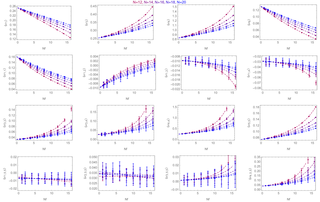
Figure 5: Mean values of the $\omega$’s plotted against $N_{f}$ for different values of $N$. Dashed lines correspond to either fits of the form $a+bN_{f}$, $a+bN_{f}+cN_{f}^{2}+dN_{f}^{3}+eN_{f}^{4}$ or $a+bN_{f}+ce^{dN_{f}}$.

Figure 5 shows plots of the $\omega$’s against $N_{f}$ for each $N$ and we fit the dependence on $N_{f}$ basically with a quartic polynomial. However, we find that higher order terms contribute for some $\omega$’s and by using the fitting function $a+bN_{f}+ce^{dN_{f}}$ we capture the dependence on $N_{f}$ over the range considered.

5 The Bosonic Berkooz-Douglas model

We are in the process of making a direct comparison of both the high-temperature regime of the BD model as determined by the above predictions and the low-temperature regime as predicted by gauge/gravity with results from a rational hybrid Monte Carlo simulation using the code used in Filev:2015cmz . We will present those results in a separate paper as, apart from their value as a check on the code and the computations presented here, they have additional physics that merits a separate discussion.

For this paper we restrict our considerations to a comparison of the results obtained here with those obtained from the bosonic Berkooz-Douglas model, whose Euclidean action is given by

$$S_{\text{bos}}=N\int_{0}^{\beta}d\tau\, \Bigg{[}\operatorname{Tr}\left(\frac{1}{2}D_{\tau}X^{a}D_{\tau}X^{a}+\frac{1}{2}D_{\tau}\bar{X}^{\rho\dot{\rho}}D_{\tau}X_{\rho\dot{\rho}}-\frac{1}{4}[X^{a},X^{b}]^{2}+\frac{1}{2}[X^{a},\bar{X}^{\rho\dot{\rho}}][X^{a},X_{\rho\dot{\rho}}]\right)$$

$$\qquad+\operatorname{tr}\left(D_{\tau}\bar{\Phi}^{\rho}D_{\tau}\Phi_{\rho}+\bar{\Phi}^{\rho}(X^{a}-m^{a})^{2}\Phi_{\rho}\right)+\frac{1}{2}\operatorname{Tr}\sum_{A=1}^{3}\mathcal{D}^{A}\mathcal{D}^{A}\Bigg{]}\,.$$ (56)

Our comparison is presented in Figure 1, where we restrict our considerations to a high precision test with $N=10$ and $N_{f}=1$. As one can see from the figure the agreement is excellent. Furthermore, the high $T$ expansion remains valid at temperatures as low as $T\sim 1.0$. Below this temperature the figure shows evidence of a phase transition. This is the phase transition of the bosonic BFSS model.

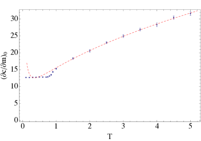
Figure 1: Comparison of the high-temperature predictions for the fundamental observable $\langle r^{2}\rangle_{\text{bos}}$ and the derivative of the condensate at zero mass, $(\partial c/\partial m)_{0}=N\langle{\mathcal{C}}^{m}\rangle_{\text{bos}}$, with a Monte Carlo simulation of the bosonic BD model. The simulation is for $N_{f}=1$ and $N=10$.

From studies of the bosonic BFSS model Filev:2015hia ; Kawahara:2007fn ; Mandal:2009vz we know that it undergoes two phase transitions at $T_{c2}=0.905\pm 0.002$ and $T_{c1}=0.8761\pm 0.0003$. These are driven by the gauge field $A$, which at high temperature behaves as one of the $X^{i}$, while at low temperature it effectively disappears from the system and can be gauged away at zero temperature. As the temperature is increased through $T_{c1}$ there is a deconfining phase transition with the symmetry $A(t)\rightarrow A(t)+\alpha{\bf 1}$ broken and the distribution of eigenvalues of the holonomy becomes non-uniform. When the temperature reaches $T_{c2}$ the spectrum of the holonomy becomes gapped and above this temperature the eigenvalues no longer cover the entire $[0,2\pi]$ range. In the low-temperature phase the bosonic BFSS model becomes a set of massive gaussian matrix models with Euclidean action

$$S_{eff}=N\int_{0}^{\beta}d\tau\operatorname{Tr}\left(\frac{1}{2}({\cal D}_{\tau}X^{i})^{2}+m_{A}^{2}(X^{i})^{2}\right)\,,$$ (57)

with the mass $m_{A}=1.965\pm 0.007$.

For the flavoured model the BFSS transition is still present and when the $X^{i}$ become massive they induce a mass for the fundamental scalars and the induced bare mass for these is estimated by integrating out the adjoint fields and expanding it to quadratic order in $\Phi_{\rho}$. This gives a mass $m_{f}^{0}=\sqrt{\frac{5}{2m_{A}}}\sim 1.128$. However, the fundamental scalars are still strongly interacting as they have a selfcoupling of order one and we expect the bare mass to become significantly dressed. We therefore estimate the physical mass of the scalars at sufficiently low temperature by assuming that they also can be described by a massive gaussian with mass $m_{f}$, in which case

$$\langle r^{2}\rangle_{\text{bos}}=\left\langle\frac{1}{\beta N_{f}}\int d\tau\,\operatorname{tr}\bar{\Phi}^{\rho}\Phi_{\rho}\right\rangle_{\text{bos}}\simeq\frac{1}{m_{f}}\,.$$ (58)

Note that the right-hand side of equation (58) is independent of $\beta$ and from Figure 1 we see that $\langle r^{2}\rangle_{\text{bos}}$ is more or less constant below the transition. A direct measurement of the expectation value (58) at $T=0.5$ gives $0.68618\simeq\frac{1}{m_{f}}$, which gives the estimate $m_{f}\simeq 1.4667$.

However, at zero temperature we can extract the masses for the different fields by measuring their Green’s function. To this end we set the holonomy to zero, the parameter $\beta$ is now just the length of the time circle and not an inverse temperature.

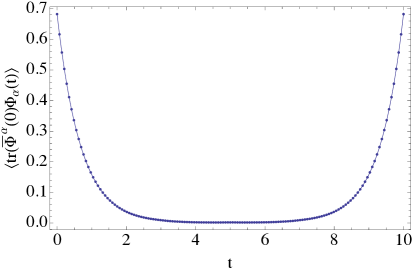
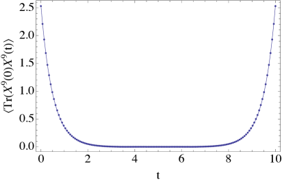
Figure 2: Plots of the Green’s functions equations (59) and (60) for $\beta=10$, $\Lambda=144$, $N=10$ and $N_{f}=1$. The fits correspond to $m_{f}=1.461$ and $m^{l}_{A}=2.001$.

Because the $SO(9)$ symmetry of the bosonic BFSS model is broken down to $SO(5)\times SO(4)$ there are now two adjoint masses, a longitudinal mass, $m_{A}^{l}$, for the four $X_{\rho\dot{\rho}}$ and a transverse mass, $m_{A}^{t}$ , for the five matrices $X^{a}$. In figure 2 we present results for the Green’s functions:

$$\langle{\rm tr}\,\bar{\Phi}^{\rho}(0)\Phi_{\rho}(\tau)\rangle = \frac{N_{f}}{m_{f}}\,\frac{e^{-m_{f}\,\tau}+e^{-m_{f}(\beta-\tau)}}{1-e^{-\beta\,m_{f}}}\ ,$$ (59)

$$\langle{\rm Tr}X^{9}(0)X^{9}(\tau)\rangle = \frac{N}{2m^{l}_{A}}\,\frac{e^{-m^{l}_{A}\,\tau}+e^{-m^{l}_{A}(\beta-\tau)}}{1-e^{-\beta\,m^{l}_{A}}}\ ,$$ (60)

where we have chosen the last of the four $SO(4)$ adjoint scalars. We have also measured the longitudinal mass $m^{l}_{A}$ by measuring the correlator for $X^{1}$ defined similarly to (60). The results for $\beta=10$, $\Lambda=144$, $N=10$ and $N_{f}=1$ are $m_{A}^{l}=2.001\pm 0.003$, $m_{A}^{t}=1.964\pm 0.003$ and $m_{f}=1.463\pm 0.001$. The prediction from assuming that the adjoint fields are described by an action of the form (57) with different masses for the transverse and longitudinal matrices is:

$$\langle R^{2}\rangle_{\text{bos}}\simeq\frac{5}{2m^{t}_{A}}+\frac{4}{2m^{l}_{A}}=2.270\pm 0.001\,,$$ (61)

which agrees well with the direct measurement where we find $\langle R^{2}\rangle_{\text{bos}}=2.261\pm 0.005$. Also the measured value of $m_{f}$ using (58) predicts that $\langle r^{2}\rangle_{\text{bos}}=0.6836\pm 0.0006$, which is in excellent agreement with the measured value.

Note that this estimate of the mass $m_{f}$ is very close to the one obtained from equation (58). Also the slightly different values of the adjoint masses $m^{t}_{A}$ and $m^{l}_{A}$ from the purely BFSS case considered in equation (57) reflect the presence of backreaction at $N_{f}/N=0.1$. Observe also the closeness of the transverse mass to the bosonic BFSS mass, which indicates that the backreaction is strongest for the longitudinal modes as one might expect.

We can now use this information to estimate the value of $\langle{\mathcal{C}}^{m}\rangle_{\text{bos}}$ at zero temperature. Assuming that both $X^{a}$ and $\Phi_{\rho}$ are well approximated by massive gaussians and using Wick’s theorem on

$$\mathcal{C}^{m}_{\text{bos}}=\frac{2}{\beta}\int_{0}^{\beta}d\tau\operatorname{tr}\bar{\Phi}^{\rho}\Phi_{\rho}-\frac{4N}{5\beta}\left(\int_{0}^{\beta}d\tau\operatorname{tr}\left\{\bar{\Phi}^{\rho}X^{a}\Phi_{\rho}\right\}\right)^{2}$$ (62)

to perform the contractions, we obtain

$$\langle{\mathcal{C}}^{m}\rangle_{\text{bos}}\Big{|}_{T=0}=\frac{2N_{f}}{m_{f}}-\frac{2N_{f}}{m_{f}^{2}m^{t}_{A}(2m_{f}+m^{t}_{A})}=1.270\pm 0.001\,.$$ (63)

Finally, a direct measurement of the measured condensate shown in Figure 1 for $T=0.4,0.3,0.2$ and $T=0.1$ extrapolated to $T=0$ gives $\langle{\mathcal{C}}^{m}\rangle_{\text{bos}}\big{|}_{T=0}=1.268\pm 0.003$, which is very close to the predicted value and confirms the validity of the gaussian approximation for both the adjoint and fundamental scalars.

6 Conclusions

We have obtained the first two terms in the high-temperature series expansion for the Berkooz-Douglas model (BD model) for general adjoint matrix size, $N$ and fundamental multiplet dimension, $N_{f}$. These results should prove useful for future studies of this model. The model is an ideal testing ground for many ideas of gauge/gravity duality. The system is strongly coupled at low temperature while at high temperature it is weakly coupled, aside from the Matsubara zero-modes, which remain strongly coupled even at high temperature. It is these modes that provide the residual non-perturbative aspect of the current study. Their effect can be captured in numerical coefficients that depend only on $N$ and $N_{f}$.

Once the coefficients are determined and tabulated (see appendix A) they can be used as input for the high-temperature expansion of the observables of the BD model. We have checked these coefficients by comparing with a high precision simulation of the bosonic version of the BD model which we simulated using the Hybrid Monte Carlo approach. The coefficients in the high-temperature expansion of the bosonic model’s observables are similarly determined by the tables presented in appendix A. In fact the observable $\langle r^{2}\rangle_{\text{bos}}$ (see equation (8)) and mass susceptibility (62) of the model, shown in Figure 1, show that the agreement is excellent even down to temperature one. Below this temperature the system undergoes a set of phase transitions. These are essentially the two phase transitions of the bosonic BFSS model.

We found that for $N_{f}/N=0.1$ our measurements were sensitive to the backreaction of the fundamental fields on the adjoint fields. This backreaction lifted the mass degeneracy of the transverse and longitudinal adjoint fields. The transverse mass was essentially unaffected by the backreaction being $m_{A}^{t}=1.964\pm 0.003$ while the longitudinal mass was lifted to $m_{A}^{l}=2.001\pm 0.003$,

We found that using our understanding of the low-temperature phase of the BFSS model as a system of massive gaussian quantum matrix models we could predict the zero-temperature value of the mass susceptibility (62). The additional input that was required was the mass of the fundamental fields which we found by direct measurement to be $m_{f}=1.463\pm 0.001$.

The zero-mode model used to obtain the high-temperature coefficients is of independent interest as it is the potential that captures the ADHM data in the theory of Yang-Mills instantons on the four-sphere, $S^{4}$. It is the bosonic sector of the dimensional reduction of the BD model to zero dimensions and is equivalent to a flavoured version of the bosonic sector of the IKKT model. For this reason we refer to the model as the flavoured bosonic IKKT model. The potential is always positive semi-definite and the Higgs branch of its zero-locus is isomorphic to the instanton moduli space Tong:2005un .

There was some evidence for peculiar behaviour in the zero mode model for $N_{f}\geq 2N$. We found that simulations required significant fine tuning for $N_{f}\geq 2N$, in that when using the same leapfrog step length which gave $95\%$ acceptance rate for $N_{f}=2N-1$ the acceptance rate for $N_{f}\geq 2N$ fell to a fraction of this within a couple of thousand sweeps and Ward identities we use as checks on the simulations were not fulfilled. After tuning the simulation we found the generated configurations had very long auto-correlation time. Also, in fitting the dependence of the observables $\Xi_{i}$ on $N$ for a given $N_{f}$ we found evidence for a simple pole at $N=2N_{f}$. Furthermore, one can see from the results tabulated in appendix A that they grow rapidly when the region $N_{f}=2N$ is approached. We expect that these difficulties and the growth of observables as $N_{f}=2N$ is approached are related to the singular structure of the instanton moduli space, i.e. the minimum of the potential in (3) with $X^{a}=0$, ${\cal D}^{A}=0$. We have not pursued this further in the current study as it would take us too far afield, however, we believe it merits further attention.

Finally, our preliminary studies of the supersymmetric BD model show in_prep that, for some observables, the high-temperature series expansion remains valid to lower temperatures than one might expect. This validity of the high $T$ expansion at lower $T$ could provide alternative quasi-analytic estimates for observables in the window where gauge/gravity duality is valid.

Appendix A Tables for the $\omega$’s.

In this appendix we gather the numerical data from Monte Carlo simulations for different matrix sizes, $N$ and different numbers of flavour multiplets $N_{f}$ and present it in tabular form.

$N_{f}=1$
$N$	$\omega_{1}$	$\omega_{3}$	$\omega_{4}$	$\omega_{6}$	$\omega_{1,1}$	$\omega_{1,2}$	$\omega_{1,3}$	$\omega_{1,4}$
4	0.2201(1)	0.26221(6)	0.8974(2)	0.0972(1)	0.130(1)	-0.0055(4)	-0.0095(6)	-0.029(2)
6	0.23428(8)	0.26207(4)	0.8749(2)	0.11105(8)	0.140(1)	-0.0068(8)	-0.0097(8)	-0.029(3)
8	0.24057(4)	0.26126(2)	0.8644(1)	0.11743(4)	0.146(1)	-0.0075(6)	-0.0097(6)	-0.029(3)
9	0.24246(3)	0.26087(2)	0.8606(1)	0.11938(4)	0.148(1)	-0.0078(7)	-0.0097(7)	-0.030(3)
10	0.243940(9)	0.260480(4)	0.85798(3)	0.120880(9)	0.1488(4)	-0.0079(2)	-0.0097(2)	-0.029(1)
12	0.24608(2)	0.25987(1)	0.8539(1)	0.12309(3)	0.151(2)	-0.0082(9)	-0.0097(9)	-0.029(5)
14	0.24756(3)	0.25933(1)	0.8512(1)	0.12461(3)	0.152(3)	-0.008(1)	-0.01(1)	-0.029(6)
16	0.24862(2)	0.258930(8)	0.8500(1)	0.12572(2)	0.154(2)	-0.009(1)	-0.01(1)	-0.029(7)
18	0.24942(2)	0.258580(9)	0.84732(8)	0.12654(2)	0.154(3)	-0.009(1)	-0.01(2)	-0.030(8)
20	0.250070(4)	0.258300(2)	0.84604(2)	0.127220(5)	0.1553(9)	-0.0087(4)	-0.0097(5)	-0.029(3)
32	0.252130(4)	0.257260(2)	0.84167(3)	0.129360(4)	0.158(2)	-0.0091(9)	-0.010(1)	-0.029(7)
$\infty$	0.25530(3)	0.25533(3)	0.8346(1)	0.13282(7)	0.1619(2)	-0.00955(4)	-0.00959(3)	-0.0288(5)

$N_{f}=1$
$N$	$\omega_{3,3}$	$\omega_{3,4}$	$\omega_{4,4}$	$\omega_{5,5}$	$\omega_{1,5,5}$	$\omega_{2,5,5}$	$\omega_{3,5,5}$	$\omega_{4,5,5}$
4	0.0403(6)	0.033(1)	0.305(2)	0.0779(1)	-0.0059(4)	0.033(1)	0.0020(5)	0.0483(6)
6	0.0372(7)	0.031(2)	0.289(2)	0.07770(8)	-0.0064(8)	0.034(1)	0.0021(8)	0.0472(6)
8	0.0361(8)	0.030(2)	0.280(2)	0.07726(9)	-0.006(1)	0.033(2)	0.002(1)	0.0461(8)
9	0.0357(7)	0.030(2)	0.277(2)	0.07710(9)	-0.007(2)	0.034(2)	0.002(2)	0.0458(9)
10	0.0355(2)	0.030(1)	0.2752(6)	0.07699(3)	-0.0065(6)	0.0344(8)	0.0020(7)	0.0455(3)
12	0.0351(8)	0.029(4)	0.272(2)	0.07665(8)	-0.006(3)	0.031(3)	0.002(3)	0.0451(9)
14	0.035(1)	0.029(5)	0.269(2)	0.07634(7)	-0.007(3)	0.035(4)	0.002(3)	0.0441(9)
16	0.035(1)	0.029(7)	0.267(3)	0.07629(8)	-0.007(5)	0.035(6)	0.002(5)	0.044(1)
18	0.034(1)	0.029(8)	0.266(3)	0.07620(7)	-0.007(6)	0.038(7)	0.002(6)	0.044(1)
20	0.0343(4)	0.028(3)	0.2648(8)	0.07599(2)	-0.006(2)	0.034(2)	0.002(2)	0.0438(3)
32	0.0340(9)	0.028(7)	0.261(1)	0.07559(2)	-0.007(5)	0.035(5)	0.002(5)	0.0430(6)
$\infty$	0.03352(6)	0.0272(1)	0.2542(1)	0.07479(6)	-0.0071(5)	0.036(2)	0.00188(6)	0.0416(2)

Table 1: Mean values of the $\omega$’s for $N_{f}=1$ were obtained from $3\times 10^{6}$ Monte Carlo samples for all values of $N$ but $10\ (3\times 10^{7}\mbox{samples})$ and $20,\ 32\ (6\times 10^{7}\mbox{samples})$. Errors are estimated with the Jackknife resampling. $N=\infty$ values are the one extrapolated by quadratic polynomials: $a+b/N+c/N^{2}$. The quoted errors of this extrapolation are the fitting errors of the parameter $a$.

In the remaining tables we tabulate fixed $N=9,12,14,16,18$ and $20$ while we vary $N_{f}$. Mean values of observable $\omega_{i}$, $\omega_{i,j}$ and $\omega_{i,j,k}$ ($i,j,k=1,...,6$) were obtained from $3\times 10^{6}$ samples generated by hybrid Monte Carlo simulation of flavoured bosonic IKKT model with the action specified in (16). Errors are estimated with the Jackknife resampling.

$N=9$
$N_{f}$	$\omega_{1}$	$\omega_{3}$	$\omega_{4}$	$\omega_{6}$	$\omega_{1,1}$	$\omega_{1,2}$	$\omega_{1,3}$	$\omega_{1,4}$
2	0.23205(3)	0.26942(2)	0.88939(9)	0.10936(3)	0.134(1)	-0.0062(7)	-0.0099(7)	-0.030(3)
4	0.21144(2)	0.28898(2)	0.95582(8)	0.09091(2)	0.1093(9)	-0.0035(5)	-0.0107(6)	-0.033(2)
6	0.19103(2)	0.31301(2)	1.03840(9)	0.07438(2)	0.0887(8)	-0.0015(4)	-0.0118(7)	-0.036(2)
8	0.17041(2)	0.34381(3)	1.1462(1)	0.05941(2)	0.0709(6)	0.0002(4)	-0.0133(6)	-0.042(2)
10	0.14909(2)	0.38552(5)	1.2945(2)	0.04570(1)	0.0551(6)	0.0016(4)	-0.0161(6)	-0.052(2)
12	0.12643(2)	0.44720(7)	1.5183(3)	0.03313(1)	0.0411(5)	0.0027(3)	-0.0208(6)	-0.070(2)
14	0.10098(3)	0.5532(2)	1.9094(7)	0.02139(1)	0.0284(5)	0.0037(4)	-0.0311(6)	-0.108(3)
16	0.06951(4)	0.8022(6)	2.838(2)	0.01036(1)	0.0165(5)	0.0045(4)	-0.0639(8)	-0.230(4)

$N=9$
$N_{f}$	$\omega_{3,3}$	$\omega_{3,4}$	$\omega_{4,4}$	$\omega_{5,5}$	$\omega_{1,5,5}$	$\omega_{2,5,5}$	$\omega_{3,5,5}$	$\omega_{4,5,5}$
2	0.0384(7)	0.034(3)	0.310(3)	0.08089(7)	-0.006(1)	0.034(2)	0.002(2)	0.053(1)
4	0.0450(8)	0.044(3)	0.397(5)	0.08971(8)	-0.007(1)	0.033(2)	0.004(2)	0.072(3)
6	0.054(1)	0.061(4)	0.54(1)	0.1015(1)	-0.007(2)	0.031(2)	0.006(3)	0.105(6)
8	0.069(2)	0.091(6)	0.78(2)	0.1179(1)	-0.008(2)	0.032(3)	0.011(3)	0.16(1)
10	0.095(3)	0.15(1)	1.25(6)	0.1423(2)	-0.010(2)	0.030(3)	0.019(5)	0.28(2)
12	0.146(5)	0.27(2)	2.3(1)	0.1816(2)	-0.014(2)	0.030(3)	0.043(8)	0.55(4)
14	0.29(2)	0.66(6)	5.5(4)	0.2527(3)	-0.021(2)	0.027(3)	0.11(2)	1.3(1)
16	1.02(8)	2.9(3)	24.(2)	0.4275(9)	-0.043(4)	0.010(5)	0.52(7)	5.6(5)

$N=12$
$N_{f}$	$\omega_{1}$	$\omega_{3}$	$\omega_{4}$	$\omega_{6}$	$\omega_{1,1}$	$\omega_{1,2}$	$\omega_{1,3}$	$\omega_{1,4}$
2	0.23828(2)	0.26610(1)	0.87476(8)	0.11545(3)	0.141(2)	-0.0069(9)	-0.010(1)	-0.029(4)
4	0.22278(2)	0.27982(1)	0.92086(7)	0.10101(2)	0.121(1)	-0.0048(7)	-0.0103(8)	-0.031(4)
6	0.20742(2)	0.29562(2)	0.97439(8)	0.08770(2)	0.104(1)	-0.0030(7)	-0.0109(9)	-0.033(3)
8	0.19209(2)	0.31413(2)	1.0380(1)	0.07536(2)	0.089(1)	-0.0015(7)	-0.0118(9)	-0.037(3)
10	0.17660(2)	0.33637(3)	1.1149(1)	0.06387(2)	0.075(1)	-0.0002(6)	-0.0130(9)	-0.041(3)
12	0.16082(2)	0.36396(3)	1.2121(1)	0.05316(1)	0.0631(8)	0.0009(5)	-0.0146(8)	-0.046(3)
14	0.14454(2)	0.39950(4)	1.3391(2)	0.04314(1)	0.0518(7)	0.0019(5)	-0.0170(8)	-0.056(3)
16	0.12733(2)	0.44796(6)	1.5145(3)	0.03368(1)	0.0414(7)	0.0027(5)	-0.0208(8)	-0.070(4)

$N=12$
$N_{f}$	$\omega_{3,3}$	$\omega_{3,4}$	$\omega_{4,4}$	$\omega_{5,5}$	$\omega_{1,5,5}$	$\omega_{2,5,5}$	$\omega_{3,5,5}$	$\omega_{4,5,5}$
2	0.0369(9)	0.032(4)	0.295(3)	0.07944(7)	-0.006(3)	0.033(3)	0.003(3)	0.050(2)
4	0.041(1)	0.039(4)	0.351(6)	0.08544(8)	-0.007(3)	0.033(3)	0.003(3)	0.062(4)
6	0.047(1)	0.048(5)	0.43(1)	0.09269(9)	-0.006(3)	0.031(4)	0.004(4)	0.079(7)
8	0.054(2)	0.061(7)	0.54(2)	0.10189(9)	-0.007(3)	0.031(3)	0.007(4)	0.11(1)
10	0.065(3)	0.082(9)	0.70(3)	0.1136(1)	-0.008(3)	0.031(4)	0.010(6)	0.15(2)
12	0.080(3)	0.11(1)	0.97(5)	0.1292(1)	-0.008(3)	0.028(3)	0.014(7)	0.21(2)
14	0.103(5)	0.17(2)	1.42(8)	0.1508(2)	-0.011(3)	0.033(4)	0.023(9)	0.32(4)
16	0.144(7)	0.27(3)	2.3(1)	0.1816(2)	-0.014(3)	0.033(4)	0.04(1)	0.54(6)

$N=14$
$N_{f}$	$\omega_{1}$	$\omega_{3}$	$\omega_{4}$	$\omega_{6}$	$\omega_{1,1}$	$\omega_{1,2}$	$\omega_{1,3}$	$\omega_{1,4}$
2	0.24085(2)	0.26461(1)	0.86849(8)	0.11800(2)	0.143(2)	-0.007(1)	-0.010(1)	-0.029(5)
4	0.22755(2)	0.27607(1)	0.90708(7)	0.10541(2)	0.127(2)	-0.0054(8)	-0.010(1)	-0.031(4)
6	0.21435(2)	0.28893(1)	0.95027(6)	0.09363(2)	0.111(2)	-0.0037(8)	-0.011(1)	-0.032(4)
8	0.20119(2)	0.30355(1)	0.99992(7)	0.08262(2)	0.098(1)	-0.0023(8)	-0.011(1)	-0.035(4)
10	0.18802(2)	0.32044(2)	1.05810(8)	0.07231(1)	0.085(1)	-0.0011(7)	-0.0121(9)	-0.038(4)
12	0.17472(1)	0.34031(2)	1.12710(8)	0.06259(1)	0.0737(9)	0.0000(6)	-0.0132(9)	-0.041(3)
14	0.16118(1)	0.36434(2)	1.21160(9)	0.05344(1)	0.0632(9)	0.0010(6)	-0.0146(9)	-0.047(3)
16	0.14723(1)	0.39416(3)	1.3179(1)	0.044771(8)	0.0536(8)	0.0018(5)	-0.0167(9)	-0.054(4)

$N=14$
$N_{f}$	$\omega_{3,3}$	$\omega_{3,4}$	$\omega_{4,4}$	$\omega_{5,5}$	$\omega_{1,5,5}$	$\omega_{2,5,5}$	$\omega_{3,5,5}$	$\omega_{4,5,5}$
2	0.036(1)	0.031(5)	0.288(4)	0.07870(8)	-0.007(4)	0.035(4)	0.003(4)	0.049(2)
4	0.040(1)	0.037(5)	0.333(7)	0.08372(7)	-0.006(3)	0.032(4)	0.003(4)	0.058(4)
6	0.044(2)	0.044(5)	0.39(1)	0.08958(9)	-0.006(4)	0.032(5)	0.004(5)	0.071(7)
8	0.050(2)	0.054(6)	0.47(2)	0.09655(8)	-0.008(3)	0.035(4)	0.005(5)	0.090(9)
10	0.057(2)	0.067(8)	0.58(2)	0.1051(1)	-0.007(4)	0.030(4)	0.007(6)	0.12(2)
12	0.066(2)	0.086(9)	0.73(3)	0.1156(1)	-0.007(4)	0.030(5)	0.010(8)	0.15(2)
14	0.080(3)	0.11(1)	0.97(4)	0.1297(1)	-0.009(4)	0.033(5)	0.015(8)	0.21(3)
16	0.099(5)	0.16(2)	1.34(8)	0.1473(1)	-0.010(4)	0.030(5)	0.02(1)	0.30(5)

$N=16$
$N_{f}$	$\omega_{1}$	$\omega_{3}$	$\omega_{4}$	$\omega_{6}$	$\omega_{1,1}$	$\omega_{1,2}$	$\omega_{1,3}$	$\omega_{1,4}$
2	0.24274(2)	0.263510(9)	0.86416(7)	0.11988(2)	0.146(2)	-0.008(1)	-0.010(1)	-0.029(6)
4	0.23108(2)	0.27333(1)	0.89680(5)	0.10870(2)	0.131(2)	-0.006(1)	-0.010(1)	-0.030(5)
6	0.21953(2)	0.28417(1)	0.93336(6)	0.09821(2)	0.117(2)	-0.004(1)	-0.010(1)	-0.031(4)
8	0.20799(2)	0.29622(1)	0.97404(6)	0.08826(1)	0.104(2)	-0.0030(9)	-0.011(1)	-0.033(5)
10	0.19650(1)	0.30983(1)	1.02060(6)	0.07890(1)	0.093(2)	-0.0018(8)	-0.012(1)	-0.036(4)
12	0.18493(1)	0.32538(2)	1.07400(7)	0.07002(1)	0.082(1)	-0.0008(8)	-0.012(1)	-0.038(5)
14	0.17325(1)	0.34335(2)	1.13660(8)	0.06159(1)	0.072(1)	0.0002(8)	-0.013(1)	-0.042(4)
16	0.16138(1)	0.36458(2)	1.2110(1)	0.05360(1)	0.063(1)	0.0010(7)	-0.015(1)	-0.047(4)

$N=16$
$N_{f}$	$\omega_{3,3}$	$\omega_{3,4}$	$\omega_{4,4}$	$\omega_{5,5}$	$\omega_{1,5,5}$	$\omega_{2,5,5}$	$\omega_{3,5,5}$	$\omega_{4,5,5}$
2	0.036(1)	0.031(5)	0.283(4)	0.07823(7)	-0.007(5)	0.035(5)	0.002(5)	0.048(2)
4	0.039(1)	0.035(5)	0.321(6)	0.08239(8)	-0.006(4)	0.032(6)	0.003(5)	0.056(5)
6	0.043(2)	0.041(6)	0.37(1)	0.08736(8)	-0.007(5)	0.037(5)	0.003(6)	0.066(8)
8	0.047(2)	0.048(6)	0.43(1)	0.09295(8)	-0.007(4)	0.033(5)	0.005(6)	0.08(1)
10	0.052(2)	0.058(8)	0.51(2)	0.0996(1)	-0.008(5)	0.036(6)	0.006(8)	0.10(2)
12	0.059(3)	0.07(1)	0.61(3)	0.1074(1)	-0.007(6)	0.033(6)	0.01(1)	0.12(2)
14	0.068(3)	0.09(1)	0.76(4)	0.1175(1)	-0.008(6)	0.031(7)	0.01(1)	0.16(3)
16	0.079(4)	0.11(2)	0.97(6)	0.1293(1)	-0.009(5)	0.034(6)	0.01(1)	0.21(4)

$N=18$
$N_{f}$	$\omega_{1}$	$\omega_{3}$	$\omega_{4}$	$\omega_{6}$	$\omega_{1,1}$	$\omega_{1,2}$	$\omega_{1,3}$	$\omega_{1,4}$
2	0.24423(2)	0.262630(8)	0.86076(7)	0.12137(2)	0.147(3)	-0.008(1)	-0.010(2)	-0.029(7)
4	0.23383(2)	0.271220(9)	0.88931(5)	0.11132(2)	0.134(3)	-0.006(1)	-0.010(1)	-0.030(6)
6	0.22352(2)	0.280600(9)	0.92072(5)	0.10180(2)	0.121(2)	-0.005(1)	-0.010(1)	-0.032(5)
8	0.21329(1)	0.29087(1)	0.95536(6)	0.09279(1)	0.110(2)	-0.004(1)	-0.011(1)	-0.033(5)
10	0.20303(1)	0.30226(1)	0.99401(6)	0.08418(1)	0.099(2)	-0.002(1)	-0.011(1)	-0.034(5)
12	0.19279(1)	0.31495(1)	1.03750(7)	0.07601(1)	0.089(2)	-0.0015(9)	-0.012(1)	-0.036(5)
14	0.18251(1)	0.32929(2)	1.08690(6)	0.06825(1)	0.080(2)	-0.0006(9)	-0.013(1)	-0.039(5)
16	0.17208(1)	0.34572(2)	1.14410(8)	0.060814(9)	0.071(1)	0.0002(8)	-0.013(1)	-0.042(5)

$N=18$
$N_{f}$	$\omega_{3,3}$	$\omega_{3,4}$	$\omega_{4,4}$	$\omega_{5,5}$	$\omega_{1,5,5}$	$\omega_{2,5,5}$	$\omega_{3,5,5}$	$\omega_{4,5,5}$
2	0.036(1)	0.030(7)	0.280(4)	0.07793(8)	-0.007(6)	0.037(7)	0.002(7)	0.047(3)
4	0.038(2)	0.034(6)	0.312(7)	0.08155(7)	-0.006(6)	0.032(7)	0.003(7)	0.054(5)
6	0.041(2)	0.039(6)	0.35(1)	0.08566(8)	-0.007(6)	0.035(7)	0.003(7)	0.063(8)
8	0.045(2)	0.045(8)	0.40(2)	0.09052(8)	-0.007(6)	0.033(6)	0.005(8)	0.07(1)
10	0.049(2)	0.052(8)	0.46(2)	0.0959(1)	-0.006(7)	0.031(8)	0.00(1)	0.09(2)
12	0.054(3)	0.06(1)	0.54(3)	0.10236(9)	-0.007(6)	0.031(7)	0.01(1)	0.11(2)
14	0.061(3)	0.07(1)	0.64(3)	0.1097(1)	-0.007(7)	0.030(8)	0.01(1)	0.13(3)
16	0.069(4)	0.09(1)	0.78(5)	0.1188(1)	-0.008(6)	0.032(7)	0.01(1)	0.16(4)

$N=20$
$N_{f}$	$\omega_{1}$	$\omega_{3}$	$\omega_{4}$	$\omega_{6}$	$\omega_{1,1}$	$\omega_{1,2}$	$\omega_{1,3}$	$\omega_{1,4}$
2	0.24535(2)	0.26193(1)	0.85819(9)	0.12249(2)	0.149(4)	-0.008(2)	-0.010(2)	-0.03(1)
4	0.23602(2)	0.26956(1)	0.88333(7)	0.11341(2)	0.136(3)	-0.006(2)	-0.010(2)	-0.031(8)
6	0.22673(2)	0.27779(1)	0.91089(6)	0.10474(2)	0.125(4)	-0.005(2)	-0.010(2)	-0.031(9)
8	0.21749(2)	0.28676(1)	0.94102(7)	0.09646(2)	0.114(3)	-0.004(2)	-0.011(2)	-0.032(8)
10	0.20828(2)	0.29653(1)	0.97400(6)	0.08855(1)	0.104(3)	-0.003(2)	-0.011(2)	-0.033(7)
12	0.19906(2)	0.30727(2)	1.01070(8)	0.08099(1)	0.095(3)	-0.002(1)	-0.011(2)	-0.036(9)
14	0.18984(2)	0.31919(2)	1.05150(9)	0.07377(1)	0.087(3)	-0.001(2)	-0.012(2)	-0.038(7)
16	0.18053(2)	0.33253(2)	1.0975(1)	0.06683(1)	0.078(2)	0.000(2)	-0.013(2)	-0.039(8)

$N=20$
$N_{f}$	$\omega_{3,3}$	$\omega_{3,4}$	$\omega_{4,4}$	$\omega_{5,5}$	$\omega_{1,5,5}$	$\omega_{2,5,5}$	$\omega_{3,5,5}$	$\omega_{4,5,5}$
2	0.035(2)	0.03(1)	0.278(6)	0.07754(8)	-0.006(8)	0.032(9)	0.002(8)	0.046(3)
4	0.038(2)	0.03(1)	0.305(9)	0.08075(7)	-0.007(7)	0.037(8)	0.003(8)	0.052(5)
6	0.040(3)	0.037(9)	0.34(1)	0.08440(8)	-0.007(7)	0.037(9)	0.002(9)	0.059(9)
8	0.043(3)	0.04(1)	0.38(2)	0.08853(8)	-0.007(7)	0.031(8)	0.004(9)	0.07(1)
10	0.047(3)	0.05(1)	0.43(2)	0.0930(1)	-0.007(8)	0.03(1)	0.00(1)	0.08(2)
12	0.051(4)	0.06(2)	0.49(4)	0.0984(1)	-0.007(8)	0.03(1)	0.01(1)	0.09(3)
14	0.056(5)	0.07(2)	0.57(5)	0.1044(1)	-0.008(9)	0.031(9)	0.01(1)	0.11(4)
16	0.062(6)	0.08(2)	0.66(7)	0.1114(1)	-0.008(9)	0.03(1)	0.01(2)	0.14(4)

Table 2: The tables for $N=9$ to $N=20$ were obtained from Monte Carlo simulations with $3\times 10^{6}$ samples and errors are estimated using Jackknife resampling.

Figure 3: Mean values of the $\omega$’s plotted against $N$ with $N_{f}=1$. Dashed lines correspond to fits of the form $a+b/N+c/N^{2}$ while vertical lines correspond to $N\rightarrow\infty$ values obtained from those fits. Errors are estimated with the Jackknife resampling. Its values are quite small and it is determined rather precisely in the tables.

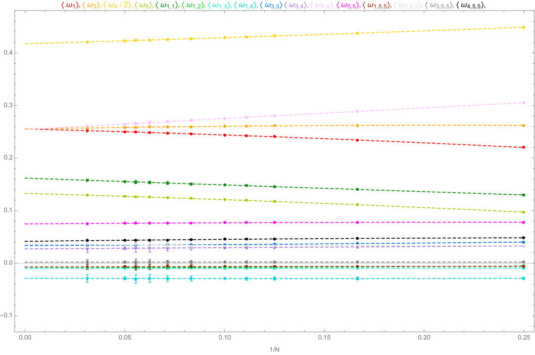
Figure 4: Mean values of the $\omega$’s plotted against $N$ with $N_{f}=1$. Dashed lines correspond to fits of the form $a+b/N$. Errors are estimated with the Jackknife resampling.

Appendix B The high-temperature behaviour of energy $E$, Polyakov loop $\langle\kern-1.0ptP\kern 1.0pt\rangle$, $\langle R^{2}\rangle$ and mass susceptibility $\langle{\mathcal{C}}^{m}\rangle$ for the supersymmetric model.

In this appendix we graphically present the high-temperature predictions for the BD-model observables the energy $E$, the Polyakov loop $\langle P\rangle$, the extent of the eigenvalues of the adjoint fields $X^{i}$ given by $\langle R^{2}\rangle$ and the mass susceptibility $\langle{\mathcal{C}}^{m}\rangle$. Figure 6 shows the predicted high-temperature behaviour of the BD-model observables.

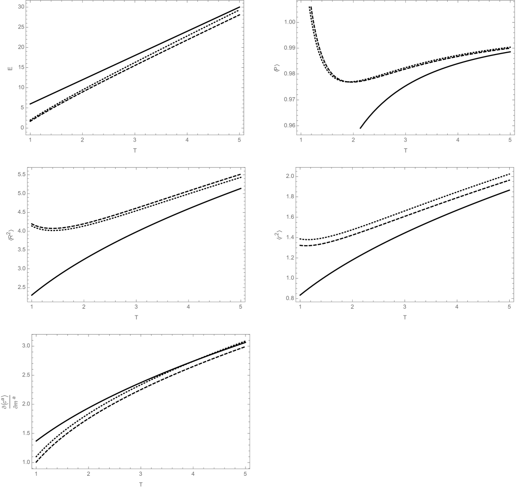
Figure 6: Temperature dependence of physical observables for the supersymmetric BD model as defined in (54) and with the values of $\omega$’s from table 1. The solid line is the leading order prediction for $N=\infty$, $N_{f}=1$ while the long dashed line is up to the next to leading order for $N=\infty$, $N_{f}=1$. The third curve with short dashes is $N=10$, $N_{f}=1$. Note that in contrast to the bosonic model the high-temperature dependence of the Polyakov loop turns upwards, as $T$ decreases, between $T=1.0$ and $2.0$. This indicates that the high-temperature series for $\langle P\rangle$ is not reliable in this region.

Figure 7: Temperature dependence of physical observables as defined in (54) with $\omega$’s from table 2 for $N=20$ and different values of $N_{f}$.

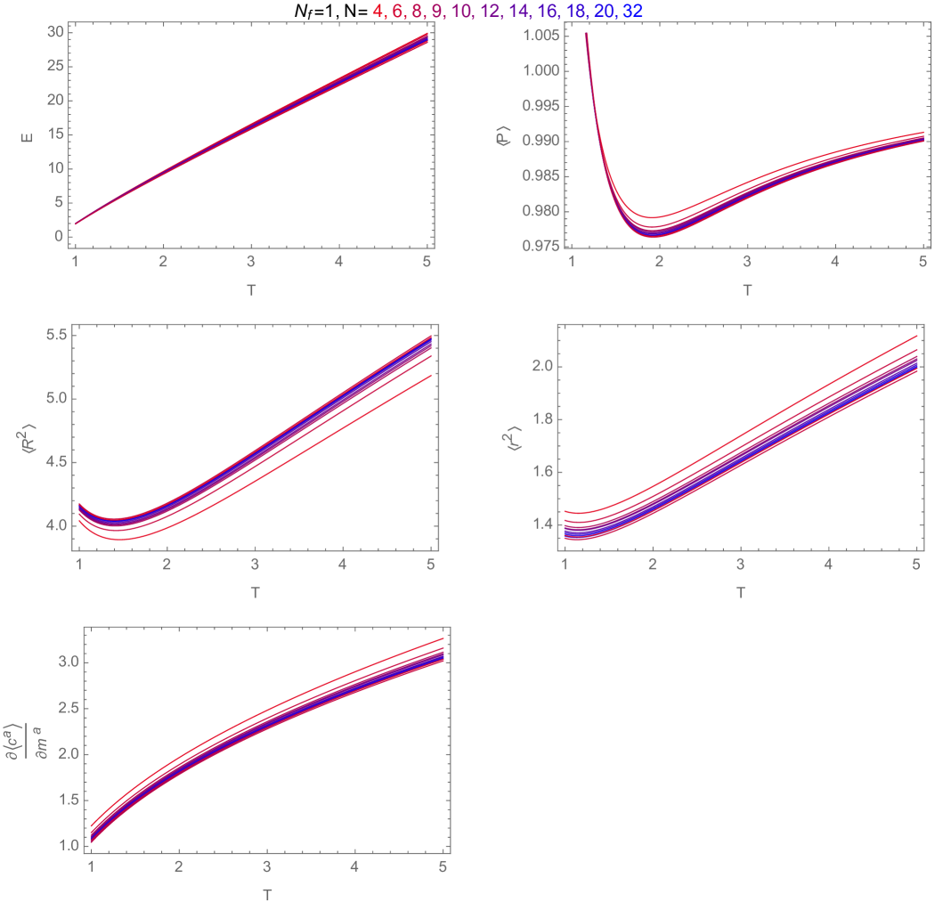
Figure 8: Temperature dependence of physical observables of the supersymmetric model as defined in (54) with $\omega$’s from table 1 for $N_{f}=1$ with different values of $N$.

Figure 9: Dependence of the energy on the temperature for the supersymmetric model as defined in (54) for $N=9,12,14,16,18,20$ with different values of $N_{f}$. Note that for each value of $N$ the curves (approximately) intersect at a crossing temperature $T_{x}$. At this point the energy is essentially independent of $N_{f}$. Extrapolating the crossing value to large $N$ we find $T_{x}=0.88\pm 0.02$, which is close to the observed transition region of the bosonic BFSS model.

References

(1)
M. Berkooz and M. R. Douglas,
“Five-branes in M(atrix) theory,”
Phys. Lett. B 395, 196 (1997)
[hep-th/9610236].
(2)
B. de Wit, J. Hoppe and H. Nicolai,
“On the Quantum Mechanics of Supermembranes,”
Nucl. Phys. B 305, 545 (1988).
(3)
T. Banks, W. Fischler, S. H. Shenker and L. Susskind,
“M theory as a matrix model: A Conjecture,”
Phys. Rev. D 55, 5112 (1997)
[hep-th/9610043].
(4)
N. Ishibashi, H. Kawai, Y. Kitazawa and A. Tsuchiya,
“A Large N reduced model as superstring,”
Nucl. Phys. B 498, 467 (1997)
[hep-th/9612115].
(5)
M. Van Raamsdonk,
“Open dielectric branes,”
JHEP 0202, 001 (2002)
[hep-th/0112081].
(6)
N. Kawahara, J. Nishimura and S. Takeuchi,
“High temperature expansion in supersymmetric matrix quantum mechanics,”
JHEP 0712, 103 (2007)
[arXiv:0710.2188 [hep-th]].
(7)
K. N. Anagnostopoulos, M. Hanada, J. Nishimura and S. Takeuchi,
“Monte Carlo studies of supersymmetric matrix quantum mechanics with sixteen supercharges at finite temperature,”
Phys. Rev. Lett. 100, 021601 (2008)
[arXiv:0707.4454 [hep-th]].
(8)
S. Catterall and T. Wiseman,
“Black hole thermodynamics from simulations of lattice Yang-Mills theory,”
Phys. Rev. D 78, 041502 (2008)
[arXiv:0803.4273 [hep-th]].
(9)
D. Kadoh and S. Kamata,
“Gauge/gravity duality and lattice simulations of one dimensional SYM with sixteen supercharges,”
[arXiv:1503.08499 [hep-lat]].
(10)
V. G. Filev and D. O’Connor,
“The BFSS model on the lattice,”
arXiv:1506.01366 [hep-th].
(11)
M. Hanada, Y. Hyakutake, G. Ishiki and J. Nishimura,
“Numerical tests of the gauge/gravity duality conjecture for D0-branes at finite temperature and finite N,”
arXiv:1603.00538 [hep-th].
(12)
A. Joseph,
“Review of Lattice Supersymmetry and Gauge-Gravity Duality,”
Int. J. Mod. Phys. A 30 (2015) no.27, 1530054
doi:10.1142/S0217751X15300549
[arXiv:1509.01440 [hep-th]].
(13)
M. Hanada,
“What lattice theorists can do for quantum gravity,”
arXiv:1604.05421 [hep-lat].
(14)
D. O’Connor and V. G. Filev,
“Membrane Matrix models and non-perturbative checks of gauge/gravity duality,”
arXiv:1605.01611 [hep-th].
(15)
V. G. Filev and D. O’Connor,
“A Computer Test of Holographic Flavour Dynamics,”
arXiv:1512.02536 [hep-th].
(16)
D. Tong,
“TASI lectures on solitons: Instantons, monopoles, vortices and kinks,”
hep-th/0509216.
(17)
M. F. Atiyah, N. J. Hitchin and I. M. Singer,
“Selfduality in Four-Dimensional Riemannian Geometry,”
Proc. Roy. Soc. Lond. A 362 (1978) 425.
doi:10.1098/rspa.1978.0143
(18)
C. Nash,
“Differential topology and quantum field theory,”
London, UK: Academic (1991) 386 p
(19)
O. Aharony, J. Marsano, S. Minwalla and T. Wiseman,
“Black hole-black string phase transitions in thermal 1+1 dimensional supersymmetric Yang-Mills theory on a circle,”
Class. Quant. Grav. 21, 5169 (2004)
doi:10.1088/0264-9381/21/22/010
[hep-th/0406210].
(20)
N. Kawahara, J. Nishimura and S. Takeuchi,
“Phase structure of matrix quantum mechanics at finite temperature,”
JHEP 0710, 097 (2007)
[arXiv:0706.3517 [hep-th]].
(21)
G. Mandal, M. Mahato and T. Morita,
“Phases of one dimensional large N gauge theory in a 1/D expansion,”
JHEP 1002, 034 (2010)
doi:10.1007/JHEP02(2010)034
[arXiv:0910.4526 [hep-th]].
(22)
B. S. DeWitt,
“Supermanifolds,” Cambridge University Press, 2nd Edition, 1992.
(23)
Y. Asano, V. G. Filev, S. Kováčik, D. O’Connor,
“A Computer Test of Holographic Flavour Dynamics II,”
arXiv:1612.09281 [hep-th].