Large Non-Gaussianity in Non-Minimally Coupled Derivative Inflation with Gauss-Bonnet Correction

Abstract

We study a nonminimal derivative inflationary model in the presence of the Gauss-Bonnet term. To have a complete treatment of the model, we consider a general form of the nonminimal derivative function and also the Gauss-Bonnet coupling term. By following the ADM formalism, expanding the action up to the third order in the perturbations and using the correlation functions, we study the perturbation and its non-Gaussian feature in details. We also study the consistency relation that gets modified in the presence of the Gauss-Bonnet term in the action. We compare the results of our consideration in confrontation with Planck2015 observational data and find some constraints on the model’s parameters. Our treatment shows that this model in some ranges of the parameters is consistent with the observational data. Also, in some ranges of model’s parameters, the model predicts blue-tilted power spectrum. Finally, we show that nonminimal derivative model in the presence of the GB term has capability to have large non-Gaussianity.

PACS numbers

04.50.Kd , 98.80.Cq , 98.80.Es

Key Words

Inflation, Cosmological Perturbations, Non-Gaussianity, Nonminimal Derivative Coupling, Observational Constraints.

I Introduction

Inflation is accepted as a paradigm of the early Universe to solve some problems of the standard big bang cosmology, such as the flatness, horizon and relics problems. An inflationary paradigm, to be a successful paradigm, should also provide a causal graceful mechanism for generating the primordial density perturbations needed to seed the formation of structures in the Universe  Gut81 ; Lin82 ; Alb82 ; Lin90 ; Lid00a ; Lid97 ; Rio02 ; Lyt09 . A simple inflationary scenario involves a single scalar field which its nearly flat potential dominated the energy density of the early Universe. Such a simple inflation model predicts the dominant mode of the primordial density fluctuations to be almost adiabatic, scale invariant and also Gaussian distributed Mal03 . However, recently released Planck observational data have detected a level of scale dependence in the primordial density perturbations Ade15a ; Ade15b . Also, Planck collaboration has obtained some constraints on the primordial non-Gaussianity in the perturbations Ade15c . Some authors have proposed extended inflationary models in light of the scalar-tensor theories which predict a level of non-Gaussianity in the density perturbation’s mode Mal03 ; Bar04 ; Che10 ; Fel11a ; Fel11b ; Noz12 ; Noz13a ; Noz13b ; Noz13c . Prediction of non-Gaussianity in the theory is really an important and impressive point, in the sense that a large amount of information about the cosmological dynamics deriving the initial inflationary expansion is carried by the non-Gaussian perturbations Bab04a ; Che08 . In this respect, it seems that such extended inflationary models are more favorable.

One successful class of the extended inflationary models in light of scalar-tensor theories, proposed by Amendola, is the one with a nonminimal coupling between the inflaton kinetic term and Einstein tensor Ame93 . By adopting such a coupling, the friction is enhanced gravitationally at higher energies, leading to increase in the friction of an inflaton rolling down its own potential. Coupling between the inflaton kinetic term and Einstein tensor which is usually given by the lagrangian term as $\left(R_{\mu\nu}-\frac{1}{2}g_{\mu\nu}R\right)\nabla^{\mu}\phi\nabla^{\nu}\phi$, satisfies the unitary invariance of the theory during inflation Ger10 . Authors have studied the early time accelerating expansion of the universe as well as the late time dynamics by considering the model with coupling between the derivatives of the scalar field and gravitational sector Tsu12 ; Sad2013 ; Sar10 ; Noz15 ; Noz14 .

Thinking over the very early Universe approaching the Planck scale, we could consider some quantum corrections on Einstein gravity. This means that Einstein gravity is a low-energy limit of a quantum theory of gravity. The most promising candidate for quantum gravity is string theory. String theory suggests that one way to accommodate quantum effects of gravity is to include quadratic curvature terms in a gravitational action as $R_{abcd}R^{abcd}-4R_{ab}R^{ab}+R^{2}$. The presence of a Gauss-Bonnet combination in the action does not have any ghost as well as any problem with the unitarity. Such a quadratic term plays a significant role in the early Universe dynamics Zwi85 ; Bou85 . However it turns out that the Gauss-Bonnet term in dimensions less than five, is a topological term having no influence in the background dynamics. In this regard, to consider the effect of the Gauss-Bonnet term on the field evolution even in four dimension, we should introduce a coupling between a scalar field and the Gauss-Bonnet term as the effective theory added to quantum correction Noj05 ; Noj07 ; Guo09 ; Guo10 (for higher dimensional extensions we refer to  Bro07 ; Bam07 ; And07 ; Noz08 ; Noz09a ; Noz09b ; Noz09c ).

In this paper, we study cosmological dynamics of a generalized inflationary model in which both the scalar field and its derivative are coupled to the curvature. The scalar field is coupled to the Gauss-Bonnet term and its derivative is coupled to the Einstein tensor. These couplings have no problem with unitarity. In this work, we consider a general form of the nonminimal derivative term in the lagrangian which includes the simple cases studied in literatures. The extended form of the nonminimal derivative term is given by ${\cal{N}}(\phi)G_{\mu\nu}\nabla^{\mu}\nabla^{\nu}(\phi)$, in which, ${\cal{N}}$ is a general function of $\phi$. This expression, for ${\cal{N}}\sim\frac{1}{2}\phi$, leads to the simple nonminimal derivative case.

To explore the viability of an inflationary model, it is important to study properties of the initial cosmological perturbations. Some parameters, such as the scalar spectral index and tensor-to-scalar ratio are important and helpful parameters to describe the main properties of the cosmological perturbations. By comparing the calculated values of the mentioned parameters in the model at hand with the observational values, we can explore whether the inflationary model is successful and viable or not. In this respect, several collaborations have tried to obtain some observational constraints on these parameters. From the joint WMAP9+eCMB+BAO+H₀ data, WMAP collaboration has obtained $r<0.13$ and $n_{s}=0.9636\pm 0.0084$ Hin13 . Planck collaboration, by using the joint Planck 2013+WMAP9+BAO data has constrained the scalar spectral index and tensor-to-scalar ratio as $r<0.12$ and $n_{s}=0.9643\pm 0.0059$ Ade13 . The new study of Planck team has released the constraints on the perturbative parameters as $r<0.099$ and $n_{s}=0.9652\pm 0.0047$, from Planck TT, TE, EE+lowP +WP data. It should be noted that Planck TT, TE, EE+lowP refer to the combination of the likelihood at $l>30$ using TT, TE, and EE spectra and the low $l$ multipole temperature polarization likelihood Ade15a ; Ade15b ; Ade15c .

With these points in mind, in section II we present the main equations of our extended inflationary model. In section III, by using the ADM formalism, we study the linear perturbations of the model at hand. In this regard, we expand the action of the model up to the second order in perturbation and consider the 2-point correlator to explore the amplitude of the scalar perturbation and also its spectral index. As well as, the tensor perturbation and its spectral index are obtained by exploring the tensor part of the perturbed metric. By considering the third order action, the non-linear perturbation in our setup is studied in section IV. In this section, by using the 3-point correlator, the non-Gaussian feature of the primordial perturbation is obtained. In the limit $k_{1}=k_{2}=k_{3}$, we compute the equilateral and orthogonal configuration of the non-Gaussianity. In section V, we examine our generalized inflationary model in confrontation with Planck2015 observational data and obtain the domain of the parameters which makes the model observationally viable.

II The Setup

The four-dimensional action for a cosmological model in the presence of a nonminimal coupling between the inflaton and the Gauss-bonnet term and a nonminimal coupling between the derivatives of the inflaton and Einstein tensor, is expressed as

$$S=\int d^{4}x\sqrt{-g}\Bigg{[}\frac{1}{2\kappa^{2}}R-\frac{1}{2}\partial_{\mu}\phi\partial^{\mu}\phi-V(\phi)-\alpha(\phi){\cal{L}_{GB}}$$

$$+{\cal{N}}(\phi)G_{\mu\nu}\nabla^{\mu}\nabla^{\nu}(\phi)\Bigg{]}\,,\hskip 17.07182pt$$ (1)

where, $R$ is the Ricci scalar, $\phi$ is an inflaton filed followed by the potential $V(\phi)$. $\alpha(\phi)$ and ${\cal{N}}(\phi)$ are general functions of the scalar field which show the nonminimal couplings. ${\cal{L}_{GB}}$ is the lagrangian of the Gauss-Bonnet term. Also, $G_{\mu\nu}$ is Einstein tensor defined as $G_{\mu\nu}=R_{\mu\nu}-\frac{1}{2}g_{\mu\nu}R$. In some papers, one see a coefficient $\frac{\kappa^{*}}{2}$, with dimension of length-squared, in front of the nonminimal derivative term. In this work, we absorb such a coefficient in nonminimal derivative function ${\cal{N}}(\phi)$. Varying the action (II) with respect to the metric, by assuming the FRW metric, leads to the following Friedmann equation of the model

$$H^{2}=\frac{\kappa^{2}}{3}\left(\dot{\phi}^{2}\Big{(}\frac{1}{2}-9H^{2}{\cal{N}}^{\prime}\Big{)}+V(\phi)+24H^{3}\dot{\alpha}\right),$$ (2)

where, a dot denotes a time derivative of the parameter and a prime refers to a derivative with respect to the inflaton field. Variation of the action (II) with respect to the scalar field, gives the equation of motion of the inflaton as follows

$$\ddot{\phi}\Big{(}-1+6{\cal{N}}^{\prime}H^{2}\Big{)}+\Big{(}12{\cal{N}}^{\prime}H\dot{H}+18{\cal{N}}^{\prime}H^{3}-3H\Big{)}\dot{\phi}$$

$$+6{\cal{N}}^{\prime\prime}H^{2}\dot{\phi}^{2}-24H^{4}\alpha^{\prime}-24H^{2}\dot{H}\alpha^{\prime}-V^{\prime}=0\,.\hskip 17.07182pt$$ (3)

In this extended inflationary model, the slow-roll parameters defined as $\epsilon\equiv-\frac{\dot{H}}{H^{2}}$ and $\eta=-\frac{1}{H}\frac{\ddot{H}}{\dot{H}}$, are given by the following expressions

$$\epsilon=\frac{E}{1+\kappa^{2}{\cal{N}}^{\prime}\dot{\phi}^{2}-8\kappa^{2}H\dot{\alpha}},$$ (4)

$$\eta=2\epsilon-\frac{\dot{E}}{H\epsilon(1+\kappa^{2}{\cal{N}}^{\prime}\dot{\phi}^{2}-8\kappa^{2}H\dot{\alpha})}$$

$$+\frac{E}{H\epsilon}\frac{\kappa^{2}{\cal{N}}^{\prime\prime}\dot{\phi}^{3}+2\kappa^{2}{\cal{N}}^{\prime}\ddot{\phi}\dot{\phi}}{(1+\kappa^{2}{\cal{N}}^{\prime}\dot{\phi}^{2}-8\kappa^{2}H\dot{\alpha})^{2}}$$

$$+\frac{E}{H\epsilon}\frac{-8\kappa^{2}H\alpha^{\prime\prime}\dot{\phi}^{2}-8\kappa^{2}H\alpha^{\prime}\ddot{\phi}-8\dot{H}\alpha^{\prime}\dot{\phi}}{(1+\kappa^{2}{\cal{N}}^{\prime}\dot{\phi}^{2}-8\kappa^{2}H\dot{\alpha})^{2}},$$ (5)

where parameter $E$ is defined as

$$E\equiv\frac{2\kappa^{2}{\cal{N}}^{\prime}\dot{\phi}\ddot{\phi}}{H}+\frac{\kappa^{2}\dot{\phi}^{2}}{2H^{2}}-3\kappa^{2}{\cal{N}}^{\prime}\dot{\phi}^{2}+\frac{\kappa^{2}{\cal{N}}^{\prime\prime}\dot{\phi}^{3}}{2H}-4\kappa^{2}\ddot{\alpha}$$

$$+4\kappa^{2}H\dot{\phi}\alpha^{\prime}\,.\hskip 14.22636pt$$ (6)

The evolution of the Hubble parameter during the inflationary era is so slow, satisfying the conditions $\epsilon\ll 1$ and $\eta\ll 1$. As one of these two slow-varying parameters reaches unity, the inflation phase of the early universe terminates.

The slow-roll limits in the simple single field inflationary model are given by $\ddot{\phi}\ll|3H\dot{\phi}|$ and $\dot{\phi}^{2}\ll V(\phi)$. In a model with NMDC and GB terms these conditions get modified. By considering the high friction regime (${\cal{N}}^{\prime}H^{2}\geq 1$), the slow-roll conditions in this setup are $8\kappa^{2}H|\dot{\alpha}|\ll 1$, $|\ddot{\alpha}|\ll|\dot{\alpha}H|$, $9H^{2}|{\cal{N}}^{\prime}|\dot{\phi}^{2}\ll V$ and $|\ddot{{\cal{N}}}|\ll|3\dot{{\cal{N}}}H^{3}|$ (the slow roll conditions in the presence of the GB term are discussed in Guo10 ; Car15 ). By using these conditions and considering $\dot{H}\ll H^{2}$ we can rewrite the Friedmann equation and equation of motion as follows

$$H^{2}\simeq\frac{\kappa^{2}}{3}V$$ (7)

$$\Big{(}18{\cal{N}}^{\prime}H^{3}-3H\Big{)}\dot{\phi}-24H^{4}\alpha^{\prime}-V^{\prime}\simeq 0\,.\hskip 17.07182pt$$ (8)

The number of e-folds during inflationary era which is defined as

$$N=\int_{t_{hc}}^{t_{f}}Hdt\,,$$ (9)

in our extended setup and within the slow-roll limits is given by the following expression

$$N\simeq\int_{\phi_{hc}}^{\phi_{f}}\frac{3H^{2}\Big{(}6{\cal{N}}^{\prime}H^{2}-1\Big{)}}{V^{\prime}+24H^{4}\alpha^{\prime}}d\phi\,,$$ (10)

In equation (10), we have shown the value of the inflaton filed at the time of the horizon crossing of the universe scale by $\phi_{hc}$ and the value of the field at the time of exit from inflationary phase by $\phi_{f}$.

We proceed by studying the linear perturbation of the model in the next section. To explore the linear perturbations, we calculate the spectrum of perturbations which are produced due to quantum fluctuations of the fields about their homogeneous background values.

III Linear Perturbations

Quantum behavior of both the scalar field $\phi$ and the space-time metric, $g_{\mu\nu}$, around their homogeneous background solution, contribute in the perturbation. In this section, we study the linear perturbation arising from fluctuation of both the scalar field and the space-time metric. To study the linear perturbation, the first step is expanding the action (II) up to the second order in small fluctuations. To this end, it is convenient to work in ADM metric formalism given by Arn60

$$ds^{2}=-N^{2}dt^{2}+h_{ij}\big{(}dx^{i}+N^{i}dt\big{)}\big{(}dx^{j}+N^{j}dt\big{)},$$ (11)

In this metric, $N^{i}$ is the shift vector and $N$ is the lapse function. By expanding the shift and laps functions as $N^{i}\equiv\Phi^{i}=\delta^{ij}\partial_{j}\Phi+v^{i}$ and $N=1+\Psi$, we obtain a general perturbed form of the metric (11). In this expansion, $\Psi$ and $\Phi$ are 3-scalars and $v^{i}$ is a vector which satisfies the condition $v^{i}_{,i}=0$ Muk92 ; Bau09 . The coefficient $h_{ij}$ is written as $h_{ij}=a^{2}\left[(1-2{\Upsilon})\delta_{ij}+2{\cal{T}}_{ij}\right]$, with ${\Upsilon}$ as the spatial curvature perturbation and ${\cal{T}}_{ij}$ as a spatial shear 3-tensor. Note that ${\cal{T}}_{ij}$ is a symmetric and traceless tensor. Now, the perturbed metric (11) is written as the following form

$$ds^{2}=-(1+2\Psi)dt^{2}+2a(t)\Phi_{i}\,dt\,dx^{i}\hskip 42.67912pt$$

$$+a^{2}(t)\left[(1-2{\Upsilon})\delta_{ij}+2{\cal{T}}_{ij}\right]dx^{i}dx^{j}.$$ (12)

Since we are going to study the scalar perturbation of the theory, it is convenient to work within the uniform-field gauge in which $\delta\phi=0$ and also the gauge ${\cal{T}}_{ij}=0$. Now, by considering the scalar part of the perturbations at the linear level and within the uniform-field gauge, the perturbed metric is given as follows  Muk92 ; Bau09 ; Bar80

$$ds^{2}=-(1+2\Psi)dt^{2}+2a(t)\Phi_{,i}\,dt\,dx^{i}\hskip 42.67912pt$$

$$+a^{2}(t)(1-2{\Upsilon})\delta_{ij}dx^{i}dx^{j}.$$ (13)

We replace the perturbed metric (III) in action (II), expand the action up to the second order in perturbations and obtain the following expression

$$S_{2}=\int dt\,d^{3}x\,a^{3}\Bigg{[}-3(\kappa^{-2}+\dot{\phi}^{2}{\cal{N}}^{\prime}-8H\dot{\alpha})\dot{\Upsilon}^{2}-\hskip 28.45274pt$$

$$\frac{2(\kappa^{-2}+\dot{\phi}^{2}{\cal{N}}^{\prime}-8H\dot{\alpha})}{a^{2}}\Psi\partial^{2}{\Upsilon}+\frac{1}{a^{2}}\Big{(}2(\kappa^{-2}+\dot{\phi}^{2}{\cal{N}}^{\prime}$$

$$-8H\dot{\alpha})\dot{\Upsilon}-\big{(}2\kappa^{-2}H+6H\dot{\phi}^{2}{\cal{N}}^{\prime}-24H^{2}\dot{\alpha}\big{)}\Psi\Big{)}\partial^{2}\Phi$$

$$+3\Big{(}2\kappa^{-2}H+6H\dot{\phi}^{2}{\cal{N}}^{\prime}-24H^{2}\dot{\alpha}\Big{)}\Psi\dot{\Upsilon}$$

$$-\Big{(}3\kappa^{-2}H^{2}-\frac{1}{2}\dot{\phi}^{2}+18H^{2}\dot{\phi}^{2}{\cal{N}}^{\prime}-48H^{3}\dot{\alpha}\Big{)}\Psi^{2}$$

$$+\frac{\kappa^{-2}+\dot{\phi}^{2}{\cal{N}}^{\prime}-8H\dot{\alpha}}{a^{2}}(\partial{\Upsilon})^{2}\Bigg{]}\,.\hskip 28.45274pt$$ (14)

By varying the action (III) in this gauge, we get the following expressions for the equations of motion of $\Psi$ and $\Phi$

$$\Psi=2\frac{\kappa^{-2}+\dot{\phi}^{2}{\cal{N}}^{\prime}-8H\dot{\alpha}}{2\kappa^{-2}H+6H\dot{\phi}^{2}{\cal{N}}^{\prime}-24H^{2}\dot{\alpha}}\dot{\Upsilon},$$ (15)

$$\frac{\partial^{2}\Phi}{a^{2}}=3\dot{\Upsilon}-\frac{\kappa^{-2}+\dot{\phi}^{2}{\cal{N}}^{\prime}-8H\dot{\alpha}}{a^{2}(2\kappa^{-2}H+6H\dot{\phi}^{2}{\cal{N}}^{\prime}-24H^{2}\dot{\alpha})}\partial^{2}{\Upsilon}$$

$$-\frac{2(3\kappa^{-2}H^{2}-\frac{1}{2}\dot{\phi}^{2}+18H^{2}\dot{\phi}^{2}{\cal{N}}^{\prime}-48H^{3}\dot{\alpha})}{(2\kappa^{-2}H+6H\dot{\phi}^{2}{\cal{N}}^{\prime}-24H^{2}\dot{\alpha})}\Psi.$$

We substitute equation of motion (15) in the second order action (III) and integrate it by parts to find

$$S_{2}=\int dt\,d^{3}x\,a^{3}{\cal{W}}\left[\dot{\Upsilon}^{2}-\frac{c_{s}^{2}}{a^{2}}(\partial{\Upsilon})^{2}\right],$$ (17)

where the parameters ${\cal{W}}$ and $c_{s}^{2}$ (known as the sound velocity) are defined as

$${\cal{W}}=-4\frac{\left(\kappa^{-2}+\dot{\phi}^{2}{\cal{N}}^{\prime}-8H\dot{\alpha}\right)^{2}\left(9\kappa^{-2}H^{2}-\frac{3}{2}\dot{\phi}^{2}+54H^{2}\dot{\phi}^{2}{\cal{N}}^{\prime}-144H^{3}\dot{\alpha}\right)}{3\left(2\kappa^{-2}H+6H\dot{\phi}^{2}{\cal{N}}^{\prime}-24H^{2}\dot{\alpha}\right)^{2}}+3\left(\kappa^{-2}+\dot{\phi}^{2}{\cal{N}}^{\prime}-8H\dot{\alpha}\right),$$ (18)

$$c_{s}^{2}=3\Bigg{[}2\Big{(}2\kappa^{-2}H+6H\dot{\phi}^{2}{\cal{N}}^{\prime}-24H^{2}\dot{\alpha}\Big{)}\Big{(}\kappa^{-2}+\dot{\phi}^{2}{\cal{N}}^{\prime}-8H\dot{\alpha}\Big{)}H-\Big{(}2\kappa^{-2}H+6H\dot{\phi}^{2}{\cal{N}}^{\prime}-24H^{2}\dot{\alpha}\Big{)}^{2}$$

$$\Big{(}\kappa^{-2}+\dot{\phi}^{2}{\cal{N}}^{\prime}-8H\dot{\alpha}\Big{)}^{-1}\Big{(}\kappa^{-2}-\dot{\phi}^{2}{\cal{N}}^{\prime}-8\ddot{\alpha}\Big{)}$$

$$+4\Big{(}2\kappa^{-2}H+6H\dot{\phi}^{2}{\cal{N}}^{\prime}-24H^{2}\dot{\alpha}\Big{)}\frac{d\Big{(}\kappa^{-2}+\dot{\phi}^{2}{\cal{N}}^{\prime}-8H\dot{\alpha}\Big{)}}{dt}$$

$$-2\Big{(}\kappa^{-2}+\dot{\phi}^{2}{\cal{N}}^{\prime}-8H\dot{\alpha}\Big{)}\,\frac{d(2\kappa^{-2}H+6H\dot{\phi}^{2}{\cal{N}}^{\prime}-24H^{2}\dot{\alpha})}{dt}\Bigg{]}\Bigg{[}\Bigg{(}9\Big{(}2\kappa^{-2}H+6H\dot{\phi}^{2}{\cal{N}}^{\prime}-24H^{2}\dot{\alpha}\Big{)}^{2}$$

$$-4\Big{(}\kappa^{-2}+\dot{\phi}^{2}{\cal{N}}^{\prime}-8H\dot{\alpha}\Big{)}\Big{(}9\kappa^{-2}H^{2}-\frac{3}{2}\dot{\phi}^{2}+54H^{2}\dot{\phi}^{2}{\cal{N}}^{\prime}-144H^{3}\dot{\alpha}\Big{)}\Bigg{)}\Bigg{]}^{-1},$$ (19)

See Refs. Fel11a ; Fel11b ; Che08 ; See05 for more details in driving this type of equations.

To proceed, we calculate the quantum perturbations of ${\Upsilon}$. In this regard, we obtain the equation of motion of ${\Upsilon}$ by varying the action (17). The result becomes

$$\ddot{\Upsilon}+\left(3H+\frac{\dot{\cal{W}}}{\cal{W}}\right)\dot{\Upsilon}+c_{s}^{2}\,\frac{k^{2}}{a^{2}}\,{\Upsilon}=0.$$ (20)

Up to the lowest order of the slow-roll approximation, solving the above equation gives

$${\Upsilon}=\frac{iHe^{-ic_{s}k\tau}}{2c_{s}^{\frac{3}{2}}\sqrt{k^{3}{\cal{W}}}}\left(1+ic_{s}k\tau\right).$$ (21)

To survey the power spectrum of the curvature perturbation, it is needed to obtain the two point correlation function in our setup. Finding the vacuum expectation value of ${\Upsilon}$ at $\tau=0$, which is corresponding to the end of inflation phase, gives the two-point correlation function as

$$\langle 0|{\Upsilon}(0,\textbf{k}_{1}){\Upsilon}(0,\textbf{k}_{2})|0\rangle=(2\pi)^{3}\delta^{3}(\textbf{k}_{1}+\textbf{k}_{2})\frac{2\pi^{2}}{k^{3}}{\cal{A}}_{s},$$ (22)

where ${\cal{A}}_{s}$, dubbed the power spectrum, is given by

$${\cal{A}}_{s}=\frac{H^{2}}{8\pi^{2}{\cal{W}}c_{s}^{3}}\,.$$ (23)

The scalar spectral index of the perturbations, which gives the scale dependence of the perturbation, at the time of the Hubble crossing is defined as

$$n_{s}-1=\frac{d\ln{\cal{A}}_{s}}{d\ln k}\Bigg{|}_{c_{s}k=aH},$$ (24)

To find the scalar spectral index in our setup, we should notice that equations (18) and (III) give

$$\kappa^{2}{\cal{W}}c_{s}^{2}=\epsilon-4\kappa^{2}H\dot{\alpha}+{\cal{O}}(\epsilon^{2})\,.$$ (25)

So, from equation (23) in the linear order we find

$${\cal{A}}_{s}=\frac{H^{2}}{8\pi^{2}(\epsilon-4\kappa^{2}H\dot{\alpha})c_{s}}\,.$$ (26)

Since $d\ln k\equiv dN=Hdt$, by using equations (24) and (26) we get

$$n_{s}-1=-2\epsilon-\frac{1}{H}\frac{d\ln(\epsilon-4\kappa^{2}H\alpha^{\prime}\dot{\phi})}{dt}$$

$$-\frac{1}{H}\frac{d\ln c_{s}}{dt}\,.\hskip 28.45274pt$$ (27)

The scale dependence of the perturbation is shown by deviation of $n_{s}$ from the unity.

Some information about the initial perturbation can be found by exploring the amplitude of the tensor perturbation and its spectral index. We should use the tensor part of the perturbed metric (III) to study the tensor perturbations. In terms of the two polarization tensors, we write ${\cal{T}}_{ij}$ as follows

$${\cal{T}}_{ij}={\cal{T}}_{+}\vartheta_{ij}^{+}+{\cal{T}}_{\times}\vartheta_{ij}^{\times},$$ (28)

In equation (28) $\vartheta_{ij}^{(+,\times)}$ are symmetric, traceless and transverse tensors. From the normalization condition we have the following constraints

$$\vartheta_{ij}^{(+,\times)}(\textbf{k})\,\vartheta_{ij}^{(+,\times)}(-\textbf{k})^{*}=2,$$ (29)

$$\vartheta_{ij}^{(+)}(\textbf{k})\,\vartheta_{ij}^{(\times)}(-\textbf{k})^{*}=0,$$ (30)

and from the reality condition we have

$$\vartheta_{ij}^{(+,\times)}(-\textbf{k})=\left(\vartheta_{ij}^{(+,\times)}(\textbf{k})\right)^{*}.$$ (31)

Now, the second order action for the tensor mode or gravitational waves becomes as follows

$$S_{T}=\int dt\,d^{3}x\,a^{3}{\cal{W}}_{T}\left[\dot{\cal{T}}_{+}^{2}-\frac{c_{\cal{T}}^{2}}{a^{2}}(\partial{\cal{T}}_{+})^{2}+\dot{\cal{T}}_{\times}^{2}-\frac{c_{\cal{T}}^{2}}{a^{2}}(\partial{\cal{T}}_{\times})^{2}\right],$$

with the parameters ${\cal{W}}_{T}$ and $c_{T}^{2}$ defined as

$${\cal{W}}_{T}=\frac{1}{4\kappa^{2}}\left(1+\kappa^{2}{\cal{N}}^{\prime}\dot{\phi}^{2}-8\kappa^{2}H\alpha^{\prime}\dot{\phi}\right),$$ (33)

$$c_{T}^{2}=1-2\kappa^{2}{\cal{N}}^{\prime}\dot{\phi}^{2}+8\kappa^{2}H\alpha^{\prime}\dot{\phi}\,.$$ (34)

To find the amplitude of the tensor perturbations we follow the strategy applied for the scalar mode case and obtain

$${\cal{A}}_{T}=\frac{H^{2}}{2\pi^{2}{\cal{W}}_{\cal{T}}c_{T}^{3}}.$$ (35)

By using equation (35) and the definition of the tensor spectral index

$$n_{T}=\frac{d\ln{\cal{A}}_{T}}{d\ln k},$$ (36)

we get the following expression for $n_{T}$ up to leading order

$$n_{T}=-2\epsilon\,.$$ (37)

Another important perturbation parameter which gives some information on the perturbation, is the ratio between the amplitudes of the tensor and scalar perturbations (briefly, tensor-to-scalar ratio). This parameter in our setup is given by the following expression

$$r=\frac{{\cal{A}}_{T}}{{\cal{A}}_{s}}\simeq 16c_{s}\left(\epsilon-4\kappa^{2}H\alpha^{\prime}\dot{\phi}\right).$$ (38)

This equation shows that the presence of the extended NMDC term, preserves the standard form of the consistency relation as $r=-8c_{s}n_{T}$. Whereas, the presence of the GB term modifies the consistency relation as equation (38).

IV Nonlinear Perturbations and Non-Gaussianity

Another important aspect of an inflationary model is given by non-Gaussianity of the primordial density perturbations. For a Gaussian distributed perturbation, all odd $n$-point correlation functions vanish and the higher even $n$-point correlators are expressed in terms of sum of products of the two-point functions. In this sense, the two-point correlation function of the scalar perturbations has no information about the non-Gaussian distribution of the primordial perturbation in the model. To explore the non-Gaussianity of the density perturbations, we should study the three-point correlation function.

In fact, every slow roll single field inflationary model with canonical kinetic term which starts from Bunch-Davies vacuum state, predicts a Gaussian distribution of the perturbations. Any deviation from these conditions leads to large non-Gaussianity. In this regard and to find the three-point correlation function, we should proceed with the nonlinear perturbation theory and expand the action (II) up to the cubic order in the small fluctuations. The result, which is a complicated expression, is shown in the Appendix A. Now, by using equation (15), we eliminate the perturbation parameter $\Psi$ in the third order action. By presenting the new parameter ${\cal{X}}$ as

$$\Phi=\frac{2(\kappa^{-2}+\dot{\phi}^{2}{\cal{N}}^{\prime}-8H\dot{\alpha}){\Upsilon}}{2\kappa^{-2}H+6\dot{\phi}^{2}H{\cal{N}}^{\prime}-24H^{2}\dot{\alpha}}\hskip 28.45274pt$$

$$+\frac{a^{2}{\cal{X}}}{\kappa^{-2}+\dot{\phi}^{2}{\cal{N}}^{\prime}-8H\dot{\alpha}}\,,\hskip 28.45274pt$$ (39)

and

$$\partial^{2}{\cal{X}}={\cal{W}}\dot{\Upsilon}\,,$$ (40)

we find the cubic action, up to the leading order, as follows

$$S_{3}=\int dt\,d^{3}x\,\Bigg{\{}\Bigg{[}\frac{3a^{3}}{\kappa^{2}c_{s}^{2}}\,\Bigg{(}1-\frac{1}{c_{s}^{2}}\Bigg{)}\Bigg{(}\epsilon-4\kappa^{2}H\dot{\alpha}\Bigg{)}\Bigg{]}{\Upsilon}\dot{\Upsilon}^{2}$$

$$+\Bigg{[}\frac{a}{\kappa^{2}}\,\Bigg{(}\frac{1}{c_{s}^{2}}-1\Bigg{)}\Bigg{(}\epsilon-4\kappa^{2}H\dot{\alpha}\Bigg{)}\Bigg{]}{\Upsilon}\,(\partial{\Upsilon})^{2}$$

$$+\Bigg{[}\frac{a^{3}}{\kappa^{2}}\,\Bigg{(}\frac{1}{c_{s}^{2}\,H}\Bigg{)}\Bigg{(}\frac{1}{c_{s}^{2}}-1\Bigg{)}\Bigg{(}\epsilon-4\kappa^{2}H\dot{\alpha}\Bigg{)}\Bigg{]}\dot{\Upsilon}^{3}$$

$$-\Bigg{[}a^{3}\,\frac{2}{c_{s}^{2}}\Bigg{(}\epsilon-4\kappa^{2}H\dot{\alpha}\Bigg{)}\dot{\Upsilon}(\partial_{i}{\Upsilon})(\partial_{i}{\cal{X}})\Bigg{]}\Bigg{\}}\,.\hskip 22.76228pt$$ (41)

At this point, by using the interacting picture, we can obtain the three point correlation function. In the interaction picture, the vacuum expectation value of the curvature perturbation $\Upsilon$ for the three-point operator is given by Mal03 ; Che08 ; See05

$$\langle{\Upsilon}(\textbf{k}_{1})\,{\Upsilon}(\textbf{k}_{2})\,{\Upsilon}(\textbf{k}_{3})\rangle=\hskip 139.41832pt$$

$$-i\int_{\tau_{i}}^{\tau_{f}}d\tau\,a\,\langle 0|[{\Upsilon}(\tau_{f},\textbf{k}_{1})\,{\Upsilon}(\tau_{f},\textbf{k}_{2})\,{\Upsilon}(\tau_{f},\textbf{k}_{3}),H_{int}(\tau)]|0\rangle,$$

which is obtained in the conformal time interval between the beginning and end of the inflation. In equation (IV), the interacting Hamiltonian, $H_{int}$, is equal to the minus of the lagrangian term of the cubic action. Given that the variation of the coefficients in the brackets of the lagrangian (IV) is slower than the scale factor, to solve the integral of equation (IV), we treat with these coefficients as constants.

Solving the integral (IV), gives the three-point correlation function in the Fourier space as the following expression

$$\langle{\Upsilon}(\textbf{k}_{1})\,{\Upsilon}(\textbf{k}_{2})\,{\Upsilon}(\textbf{k}_{3})\rangle=\hskip 99.58464pt$$

$$(2\pi)^{3}\delta^{3}(\textbf{k}_{1}+\textbf{k}_{2}+\textbf{k}_{3})B_{\Upsilon}(\textbf{k}_{1},\textbf{k}_{2},\textbf{k}_{3})\,,$$ (43)

where

$$B_{\Upsilon}(\textbf{k}_{1},\textbf{k}_{2},\textbf{k}_{3})=\frac{(2\pi)^{4}{\cal{A}}_{s}^{2}}{\prod_{i=1}^{3}k_{i}^{3}}\,{\cal{J}}_{\Upsilon}(\textbf{k}_{1},\textbf{k}_{2},\textbf{k}_{3}).$$ (44)

The parameter ${\cal{J}}_{\Upsilon}$ is given by the following expression

$${\cal{J}}_{\Upsilon}=\frac{3}{4}\Bigg{(}1-\frac{1}{c_{s}^{2}}\Bigg{)}\zeta_{1}-\frac{1}{4}\Bigg{(}1-\frac{1}{c_{s}^{2}}\Bigg{)}\zeta_{2}$$

$$+\frac{3}{2}\Bigg{(}\frac{1}{c_{s}^{2}}-1\Bigg{)}\zeta_{3},$$ (45)

where

$$\zeta_{1}=\frac{2}{K}\sum_{i>j}k_{i}^{2}\,k_{j}^{2}-\frac{1}{K^{2}}\sum_{i\neq j}k_{i}^{2}\,k_{j}^{3}\,,$$ (46)

$$\zeta_{2}=\frac{1}{2}\sum_{i}k_{i}^{3}+\frac{2}{K}\sum_{i>j}k_{i}^{2}\,k_{j}^{2}-\frac{1}{K^{2}}\sum_{i\neq j}k_{i}^{2}\,k_{j}^{3}\,,$$ (47)

$$\zeta_{3}=\frac{\left(k_{1}\,k_{2}\,k_{3}\right)^{2}}{K^{3}}\,,$$ (48)

and

$$K=k_{1}+k_{2}+k_{3}\,.$$ (49)

Equation (44) shows the dependence of the three-point correlator on the three momenta $k_{1}$ , $k_{2}$ and $k_{3}$. Satisfying the translation invariance implies that these momenta form a closed triangle which means that there should be a constraint on the momenta as $k_{1}+k_{2}+k_{3}=0$. Discussion on the issue of the shapes of the triangle is raised when one considers the translation invariance Bab04a ; Kom05 ; Cre06 ; Lig06 ; Yad07 . Depending on the amount of momenta, we are faced with different shapes of triangle. For each shapes, there is a maximal signal in a specific configuration of triangle. When there is a maximal signal in the squeezed limit with $k_{3}\ll k_{1}\simeq k_{2}$), the corresponding shape is a local shape Gan94 ; Ver00 ; Wan00 ; Kom01 . Another shape which has a signal at $k_{1}=k_{2}=k_{3}$ is called equilateral triangle Bab04b . A shape corresponding to folded triangle is given by a linear combination of the equilateral and orthogonal templates. The folded triangle is orthogonal to the equilateral triangle Sen10 and has a maximal signal in $k_{1}=2k_{2}=2k_{3}$ limit. There is a shape of non-Guassianity with a positive signal at the equilateral configuration and a negative signal at the folded configuration which is dubbed the orthogonal configuration. To measure the amplitude of the non-Gaussianity we use the dimensionless parameter $f_{{}_{NL}}$, expressed as

$$f_{NL}=\frac{10}{3}\frac{{\cal{J}}_{\Upsilon}}{\sum_{i=1}^{3}k_{i}^{3}}\,.$$ (50)

which is called “nonlinearity parameter”.

In this paper, we investigate the equilateral and orthogonal configurations of the non-Gaussianity. In this regard and to find parameter ${\cal{J}}_{\Upsilon}$ in these configurations, we follow Refs. Fer09 ; Fel13 ; Byr14 and by considering ${\cal{J}}_{\Upsilon}=\sum_{i=1}^{3}{\cal{J}}_{\Upsilon}^{(i)}$, we introduce quantity ${\cal{C}}$ by the following expression

$${\cal{C}}(\check{B}_{\Upsilon}^{(i)}\check{B}_{\Upsilon}^{(j)})=\frac{{\cal{Z}}(\check{B}_{\Upsilon}^{(i)}\check{B}_{\Upsilon}^{(j)})}{\sqrt{{\cal{Z}}(\check{B}_{\Upsilon}^{(i)}\check{B}_{\Upsilon}^{(i)}){\cal{Z}}(\check{B}_{\Upsilon}^{(i)}\check{B}_{\Upsilon}^{(i)})}}$$ (51)

where, $\check{B}_{\Upsilon}=\frac{B_{\Upsilon}}{{\cal{A}}_{s}^{2}}$ and

$${\cal{Z}}(\check{B}_{\Upsilon}^{(i)},\check{B}_{\Upsilon}^{(j)})\hskip 145.10922pt$$

$$=\int dk_{1}\,dk_{2}\,dk_{3}\,\check{B}_{\Upsilon}^{(i)}(k_{1},k_{2},k_{3})\check{B}_{\Upsilon}^{(j)}(k_{1},k_{2},k_{3})w$$ (52)

in which $w=\frac{(k_{1}k_{2}k_{3})^{4}}{(k_{1}+k_{2}+k_{3})^{3}}$. The momentum interval of integration is $0<k_{1}<\infty$, $0\leq\frac{k_{2}}{k_{1}}<1$ and $1-\frac{k_{2}}{k_{1}}\leq\frac{k_{3}}{k_{1}}\leq 1$. Every two shapes for which the constraint $|{\cal{C}}(\check{B}_{\Upsilon}\check{B}^{\prime}_{\Upsilon})|\simeq 0$ is satisfied, are almost orthogonal. In this point, we introduce a shape $\breve{\zeta}^{equil}$ as follows Fel13 ; Noz14

$$\breve{\zeta}^{equil}=-\frac{12}{13}\Big{(}3\zeta_{1}-\zeta_{2}\Big{)}\,.$$ (53)

By using equations (44), (IV), (51) and (IV), it can be shown that the following shape is orthogonal to (51)

$$\breve{\zeta}^{ortho}=\frac{12}{14-13\beta}\Big{(}\beta\big{(}3\zeta_{1}-\zeta_{2}\big{)}+3\zeta_{1}-\zeta_{2}\Big{)}\,,$$ (54)

where $\beta\simeq 1.1967996$. Now, the bispectrum (IV), in terms of the equilateral and orthogonal shapes basis is given by the following expression

$${\cal{J}}_{\Upsilon}={\cal{M}}_{1}\,\breve{\zeta}^{equil}+{\cal{M}}_{2}\,\breve{\zeta}^{ortho}\,,$$ (55)

where the parameters ${\cal{M}}_{1}$ and ${\cal{M}}_{2}$ are defined as

$${\cal{M}}_{1}=\frac{13}{12}\Bigg{[}\frac{1}{24}\bigg{(}1-\frac{1}{c_{s}^{2}}\bigg{)}\bigg{(}2+3\beta\bigg{)}\Bigg{]}\,,$$ (56)

and

$${\cal{M}}_{2}=\frac{14-13\beta}{12}\Bigg{[}\frac{1}{8}\bigg{(}1-\frac{1}{c_{s}^{2}}\bigg{)}\Bigg{]}\,.$$ (57)

The amplitudes of the non-Gaussianity in the equilateral and orthogonal configurations, obtained from equations (50)-(57), are given by

$$f_{{}_{NL}}^{equil}=\frac{130}{36\sum_{i=1}^{3}k_{i}^{3}}\Bigg{[}\frac{1}{24}\bigg{(}1-\frac{1}{c_{s}^{2}}\bigg{)}\bigg{(}2+3\beta\bigg{)}\Bigg{]}\breve{\zeta}^{equil}\,,$$ (58)

and

$$f_{{}_{NL}}^{ortho}=\frac{140-130\beta}{36\,\sum_{i=1}^{3}k_{i}^{3}}\Bigg{[}\frac{1}{8}\bigg{(}1-\frac{1}{c_{s}^{2}}\bigg{)}\Bigg{]}\breve{\zeta}^{ortho}\,.$$ (59)

Now, we rewrite equations (58) and (59) in the limit $k_{1}=k_{2}=k_{3}$ as

$$f_{{}_{NL}}^{equil}=\frac{325}{18}\Bigg{[}\frac{1}{24}\bigg{(}\frac{1}{c_{s}^{2}}-1\bigg{)}\bigg{(}2+3\beta\bigg{)}\Bigg{]}\,,$$ (60)

and

$$f_{{}_{NL}}^{ortho}=\frac{10}{9}\Big{(}\frac{65}{4}\beta+\frac{7}{6}\Big{)}\Bigg{[}\frac{1}{8}\bigg{(}1-\frac{1}{c_{s}^{2}}\bigg{)}\Bigg{]}\,.$$ (61)

This is because, there is a negative signal for the equilateral and a positive signal for an orthogonal shape function at this limit.

Up to this point, the main equations describing the cosmological dynamics of our setup, have been calculated. To investigate the cosmological viability of the model, we compare the results of our setup with the Planck2015 released data.

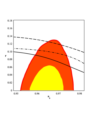
Figure 2: Tensor-to-scalar ratio versus the scalar spectral index for a NMDC inflationary model with GB coupling term, in the background of Planck2015 TT, TE, EE+lowP data. The solid line is corresponding to $n=2$. The dashed-dotted line is corresponding to $n=3$. The dashed line is corresponding to $n=4$. The diagrams have been plotted with $N=60$.

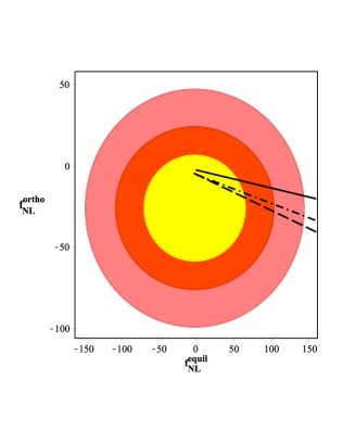
Figure 4: Amplitude of the orthogonal configuration of the non-Gaussianity versus the equilateral configuration for a NMDC inflationary model with GB coupling term, in the background of Planck2015 TTT, EEE, TTE and EET data. The solid line is corresponding to $n=2$. The dashed-dotted line is corresponding to $n=3$. The dashed line is corresponding to $n=4$. The diagrams have been plotted with $N=60$.

Table 1: The ranges of $\alpha_{{}_{0}}$ for which the values of the inflationary parameters $r$, $n_{s}$, $f_{NL}^{ortho}$ and $f_{NL}^{equil}$ are compatible with the $95\%$ CL of the Planck2015 dataset.

	$n=2$		$n=3$		$n=4$
$r-n_{s}$	$0.138<\alpha_{0}<0.285$		$0.176<\alpha_{0}<0.34$		$0.217<\alpha_{0}<0.41$
$f_{NL}^{ortho}-f_{NL}^{equil}$	$\alpha_{0}<0.13$		$\alpha_{0}<0.21$		$\alpha_{0}<0.32$

V Observational Constraints

In this section we turn our attention to the numerical analysis of the model at hand and compare it with the observational data. In this regard, we adopt the functions of scalar field, introduced in action (II), as ${\cal{N(\phi)}}\sim\frac{1}{2n}\phi^{n}$, $\alpha(\phi)\sim\alpha_{0}\phi^{n}$ and $V(\phi)\sim\frac{1}{n}\phi^{n}$. By these adoption of the general functions, we do perform our numerical analysis and obtain some constraints on the parameters space of the model. To this end, first of all, we should substitute these functions into the integral of equation (10) and solve this integral to find the value of the inflaton at the horizon crossing of the physical scales. Next, we substitute the obtained value of the field, $\phi_{hc}$, in equations (III), (38), (60) and (61). In this way, we get the scalar spectral index, tensor-to-scalar ratio, the amplitudes of the orthogonal and equilateral configurations of the non-Gaussianity in terms of $N$, $n$ and $\alpha_{0}$. Other constant parameters are rescalled to the unity. Now , we are in the situation that we can start exploring the cosmological observable parameters numerically. We perform our computation by taking $N=60$ and observational parameters are defined at $k_{0}=0.002Mpc^{-1}$ (subscript $0$ means the value of $k$ at hc). The results are shown in Figures  LABEL:fig1-4. Figure LABEL:fig1 shows the ranges of the parameters $\alpha_{0}$ and $n$ which lead to the observationally viable values of the scalar spectral index (left panel) and the tensor-to-scalar ratio (right panel). Figure shows that the NMDC model in the presence of the GB effect, in some regions of the $\alpha_{0}$ and $n$, is consistent with the Planck2015 dataset. By increasing the value of $n$, the model with stronger coupling of GB term is cosmologically viable. The interesting point is that this model, for some values of $n$ and GB coupling term, predicts blue-tilted spectrum ($n_{s}>1$). Also for this case by increasing $n$, a larger region of $\alpha_{0}$ results the blue spectrum. However, as the figure shows, a stronger GB coupling leads to red-tilted spectrum. In figure 2, we have plotted the tensor-to-scalar ratio versus the scalar spectral index in the background of the Planck2015 TT, TE, EE+lowP data. In this plot we have set $n=2$, $3$ and $4$ and performed our analysis with these values. Our analysis shows that with $n=2$, the model is consistent with observational data if $0.138<\alpha_{0}<0.285$. With $n=3$, the model has cosmological viability if $0.176<\alpha_{0}<0.34$. With $n=4$, the model is compatible with Planck2015 dataset if $0.217<\alpha_{0}<0.41$. The numerical analysis on the non-Gaussian feature of the perturbation has been studied too. The results are shown in figures LABEL:fig3 and 4. Figure LABEL:fig3 shows the range of the parameters $\alpha_{0}$ and $n$ in which the orthogonal configuration of non-Gaussianity (left panel) and the equilateral configuration of non-Gaussianity (right panel) are observationally viable. Figure 4 shows the orthogonal configuration versus the equilateral configuration of non-Gaussianity in the background of Planck2015 TTT, EEE, TTE and EET data. In this case also, we have considered three values of $n$ as $n=2$, $3$ and $4$. The corresponding diagrams are too close to be distinguished. However, in the right panel of figure 4, we have re-scaled and enlarged the plot in order to have more resolution in diagrams. By studying the behavior of the configurations of the non-Gaussianity, we have obtained some constraint on the GB coupling term. With $n=2$, the observational viability of the model is preserved if $\alpha_{0}<0.13$. With $n=3$, the numerical analysis gives the constraint as $\alpha_{0}<0.21$. With $n=4$, the model has consistency with observational data if $\alpha_{0}<0.32$. The numerical results of this section are summarized in table 1.

VI Summary

In this paper, we have considered an inflationary model in which both the inflaton scalar field and its derivatives are coupled nonminimally to gravity. The scalar field is coupled to the Gauss-Bonnet term and its derivatives are coupled to the Einstein tensor term. These coupling have no problem with unitary. First of all, we have found main equations of the inflationary dynamics in this model. Then, we have focused on the primordial perturbation in this model. In this regard, we have considered ADM formalism and carried out our computations. We have expanded the action of the model at hand, up to the second order in the perturbations and by using the two point correlator. Then we have obtained the power spectrum of the scalar perturbation and its spectral index. The power spectrum of the tensor perturbation also has been computed. We have considered the consistency relation in this setup and found that in the presence of the Gauss-bonnet coupling, the consistency relation gets modified. After that, by expanding the action up to the third order in the perturbations and using the three point correlation function we have studied the non-Gaussian feature of the perturbations. In this regard, we have presented two shape functions given by $\breve{\zeta}^{equil}$ and $\breve{\zeta}^{ortho}$ and by that we have computed the amplitude of the non-Gaussianity in the orthogonal and equilateral configurations in the limit $k_{1}=k_{2}=k_{3}$, in which both configuration have peak. To test the cosmological viability of this setup, in the section V, we have compared the results of this model in confrontation with Planck2015 observational data. To this end, by adopting ${\cal{N(\phi)}}\sim\frac{1}{2n}\phi^{n}$, $\alpha(\phi)\sim\alpha_{0}\phi^{n}$ and $V(\phi)\sim\frac{1}{n}\phi^{n}$, we have plotted the region of $\alpha_{0}$ and $n$ which lead to the observationally viable values of $n_{s}$ and $r$. We have found that NMDC model with a GB coupling in some ranges of the parameters space is consistent with Planck2015 observational data. By increasing the value of $n$, more stronger coupling of the Gauss-Bonnet term is needed to model be fitted with observation. A notable point is that this model in some ranges of the parameters predicts blue-tilted power spectrum. As $n$ increases, the model in larger region of $n$ and $\alpha_{0}$ is consistent with the Planck2015 dataset. As GB coupling becomes stronger, the model tends to the red-tilted power spectrum. The tensor-to-scalar ratio versus the scalar spectral index in the background of Planck2015 TT, TE, EE+lowP data has been plotted and some constraints on the GB coupling parameter $\alpha_{0}$ have been obtained. The non-Gaussian feature of the perturbation also in this model has been studied. The range of the cosmologically viable $n$ and $\alpha_{0}$ have been plotted. By plotting the orthogonal configuration versus the equilateral configuration of the non-Gaussianity in the background of Planck2015 TTT, EEE, TTE and EET data, some constraints on the model’s parameters are obtained. This extended inflationary model in some ranges of $n$ and $\alpha_{0}$ predicts large non-Gaussianity. In fact, we expect large non-Gaussianity in this model as a result of non-canonical kinetic term in the lagrangian. Also, in the presence of the GB term, this model is not a single-field inflationary model anymore. Consequently, this model has capability to predict large non-Gaussianity.

Appendix A The expanded action up to third order

$$S_{3}=\int dt\,d^{3}x\,a^{3}\Bigg{[}\left(3\kappa^{-2}H^{2}-\frac{\dot{\phi}^{2}}{2}+30H^{2}\dot{\phi}^{2}{\cal{N}}^{\prime}-80H^{3}\dot{\alpha}\right)\Psi^{3}+\Psi^{2}\Bigg{(}\Big{(}\frac{3}{2}\dot{\phi}^{2}-9\kappa^{-2}H^{2}+144H^{3}\dot{\alpha}-54H^{2}\dot{\phi}^{2}{\cal{N}}^{\prime}\Big{)}{\Upsilon}$$

$$+\Big{(}-6\kappa^{-2}H-36H\dot{\phi}^{2}{\cal{N}}^{\prime}+144H^{2}\dot{\alpha}\Big{)}\dot{\Upsilon}+\left(2\dot{\phi}^{2}{\cal{N}}^{\prime}-16H\dot{\alpha}\right)\frac{\partial^{2}{\Upsilon}}{a^{2}}+\Big{(}-2\kappa^{-2}H+12H\dot{\phi}^{2}{\cal{N}}^{\prime}+48H^{2}\dot{\alpha}\Big{)}\frac{\partial^{2}\Phi}{a^{2}}\Bigg{)}$$

$$+\Psi\Bigg{(}-a^{-2}\Big{(}2\kappa^{-2}H+6\dot{\phi}^{2}{\cal{N}}^{\prime}-24H^{2}\dot{\alpha}\Big{)}\partial_{i}{\Upsilon}\partial_{i}\Phi+9\Big{(}2\kappa^{-2}H+6\dot{\phi}^{2}{\cal{N}}^{\prime}-24H^{2}\dot{\alpha}\Big{)}\dot{\Upsilon}{\Upsilon}+\frac{16\dot{\alpha}}{a^{2}}\dot{\Upsilon}\partial^{2}\Upsilon$$

$$-\frac{\kappa^{-2}+3\dot{\phi}^{2}{\cal{N}}^{\prime}-12H\dot{\alpha}}{2a^{4}}\Big{(}\partial_{i}\partial_{j}\Phi\partial_{i}\partial_{j}\Phi-\partial^{2}\Phi\partial^{2}\Phi\Big{)}+\frac{16\dot{\alpha}}{a^{4}}\Big{(}\partial_{i}\partial_{j}\Phi\,\partial_{i}\partial_{j}\Upsilon-\partial^{2}\Phi\,\partial^{2}\Upsilon\Big{)}-2\frac{\kappa^{-2}+\dot{\phi}^{2}{\cal{N}}^{\prime}-8H\dot{\alpha}}{a^{2}}{\Upsilon}\partial^{2}{\Upsilon}$$

$$-\frac{2\kappa^{-2}H+6\dot{\phi}^{2}{\cal{N}}^{\prime}-24H^{2}\dot{\alpha}}{a^{2}}{\Upsilon}\partial^{2}\Phi-\frac{2\kappa^{-2}+6\dot{\phi}^{2}{\cal{N}}^{\prime}-48H\dot{\alpha}}{a^{2}}\dot{\Upsilon}\partial^{2}\Phi-\frac{\kappa^{-2}+\dot{\phi}^{2}{\cal{N}}^{\prime}-8H\dot{\alpha}}{a^{2}}(\partial{\Upsilon})^{2}$$

$$+\Big{(}3\kappa^{-2}+9\dot{\phi}^{2}{\cal{N}}^{\prime}+72H\dot{\alpha}\Big{)}\dot{\Upsilon}^{2}\Bigg{)}+8\dot{\alpha}\dot{\Upsilon}^{3}+\frac{\kappa^{-2}-\dot{\phi}^{2}{\cal{N}}^{\prime}-8\ddot{\alpha}}{a^{2}}{\Upsilon}(\partial{\Upsilon})^{2}-9\Big{(}\kappa^{-2}+\dot{\phi}^{2}{\cal{N}}^{\prime}-8H\dot{\alpha}\Big{)}\dot{\Upsilon}^{2}\,{\Upsilon}$$

$$+2\frac{\kappa^{-2}+\dot{\phi}^{2}{\cal{N}}^{\prime}-8H\dot{\alpha}}{a^{2}}\dot{\Upsilon}\partial_{i}{\Upsilon}\partial_{i}\Phi-\frac{8\dot{\alpha}}{a^{2}}\dot{\Upsilon}^{2}\partial^{2}\Phi+2\frac{\kappa^{-2}+\dot{\phi}^{2}{\cal{N}}^{\prime}-8H\dot{\alpha}}{a^{2}}\dot{\Upsilon}{\Upsilon}\partial^{2}\Phi$$

$$+\frac{\frac{3}{2}\Big{(}\kappa^{-2}+\dot{\phi}^{2}{\cal{N}}^{\prime}-8H\dot{\alpha}\Big{)}{\Upsilon}-4\dot{\alpha}\dot{\Upsilon}}{a^{4}}\Big{(}\partial_{i}\partial_{j}\Phi\partial_{i}\partial_{j}\Phi-\partial^{2}\Phi\partial^{2}\Phi\Big{)}-2\frac{\kappa^{-2}+\dot{\phi}^{2}{\cal{N}}^{\prime}-8H\dot{\alpha}}{a^{4}}\partial_{i}{\Upsilon}\partial_{i}\Phi\,\partial^{2}\Phi\Bigg{]}$$

References

- (1) A. Guth, Phys. Rev. D, 23, 347 (1981).
- (2) A. D. Linde, Phys. Lett. , 108 B, 389 (1982)
- (3) A. Albrecht and P. Steinhard, Phys. Rev. D, 48, 1220 (1982).
- (4) A. D. Linde, Particle Physics and Inflationary Cosmology (Harwood Academic Publishers, Chur, Switzerland, 1990). [arXiv:hep-th/0503203].
- (5) A. Liddle and D. Lyth, Cosmological Inflation and Large-Scale Structure, (Cambridge University Press, 2000).
- (6) J. E. Lidsey et al, Abney, Rev. Mod. Phys., 69, 373, (1997).
- (7) A. Riotto, [arXiv:hep-ph/0210162].
- (8) D. H. Lyth and A. R. Liddle, The Primordial Density Perturbation (Cambridge University Press, 2009).
- (9) J. M. Maldacena, JHEP, 0305, 013, (2003).
- (10) P. A. R. Ade et al., [arXiv:1502.02114] [astro-ph.CO].
- (11) P. A. R. Ade et al., [arXiv:1502.01589] [astro-ph.CO].
- (12) P. A. R. Ade et al., [arXiv:1502.01592] [astro-ph.CO].
- (13) N. Bartolo, E. Komatsu, S. Matarrese and A. Riotto, Phys.Rept., 402, 103, (2004).
- (14) X. Chen, Adv. Astron. 2010, 638979, (2010).
- (15) A. De Felice and S. Tsujikawa, Phys. Rev. D, 84, 083504, (2011).
- (16) A. De Felice and S. Tsujikawa, JCAP, 1104, 029, (2011).
- (17) K. Nozari and N. Rashidi, Phys. Rev. D, 86, 043505 (2012).
- (18) K. Nozari and N. Rashidi, Phys. Rev. D, 88, 023519 (2013).
- (19) K. Nozari and N. Rashidi, Phys. Rev. D, 88, 084040 (2013).
- (20) K. Nozari and N. Rashidi, Astrophys. Space Sci. 350, 339 (2014).
- (21) D. Babich, P. Creminelli and M. Zaldarriaga, JCAP, 0408, 009, (2004).
- (22) C. Cheung, P. Creminelli, A. L. Fitzpatrick, J. Kaplan and L. Senatore, JHEP, 0803, 014, (2008).
- (23) L. Amendola, Phys. Lett. B, 301, 175, (1993).
- (24) C. Germani and A. Kehagias, Physical Review Letters, 105, 011302, (2010).
- (25) S. Tsujikawa, Physical Review D, 85, 083518, (2012).
- (26) H. M. Sadjadi and P. Goodarzi, JCAP, 02, article 038, (2013).
- (27) E. N. Saridakis and S. V. Sushkov, Physical Review D, 81, 083510, (2010).
- (28) K. Nozari and N. Rashidi, Arxiv:1509.06240.
- (29) K. Nozari, M.shoukrani and N. rashidi, Advances in High Energy Physics, 2014, 343819, http://dx.doi.org/10.1155/2014/343819, (2014)
- (30) B. Zwiebach, Phys. Lett. B, 156, 315, (1985).
- (31) D. G. Boulware and S. Deser, Phys. Rev. Lett. , 55, 2656, (1985).
- (32) S. Nojiri, S. D. Odintsov and M. Sasaki, Phys. Rev. D, 71, 123509, (2005).
- (33) S. Nojiri, S. D. Odintsov and P. V. Tretyakov, Phys. Lett. B, 651, 224, (2007).
- (34) Z. K. Guo and D. J. Schwarz, Phys. Rev. D, 80, 063523, (2009).
- (35) Z. K. Guo and D. J. Schwarz, Phys. Rev. D, 81, 123520, (2010).
- (36) R. A. Brown, Brane world cosmology with Gauss-Bonnet and induced gravity terms, (PhD Thesis, 2007), [arXiv:gr-qc/0701083].
- (37) K. Bamba, Z. K. Guo and N. Ohta, Prog. Theor. Phys., 118, 879, (2007).
- (38) K. Andrew, B. Bolen and C. A. Middleton, Gen. Rel. Grav., 39, 2061, (2007).
- (39) K. Nozari and B. Fazlpour, JCAP, 0806, 032, (2008).
- (40) K. Nozari, and N. Rashidi, Int. J. Thoer. Phys., 48, 2800, (2009).
- (41) K. Nozari, and N. Rashidi, JCAP, 0909, 014, (2009).
- (42) K. Nozari, and N. Rashidi, Int. J. Mod. Phys. D, 19, 219, (2009).
- (43) G. Hinshaw et al., Astrophys. J. Suppl. Ser. 208, 19 (2013).
- (44) P. A. R. Ade et al., arXiv:1303.5082.
- (45) C. van de Bruck and C. Longden, arXiv:1512.04768.
- (46) R. L. Arnowitt, S. Deser and C. W. Misner, Phys. Rev., 117, 1595, (1960).
- (47) V. F. Mukhanov, H. A. Feldman, R. H. Brandenberger, Physics Reports, 215, 203, (1992).
- (48) Daniel Baumann, [arXiv:0907.5424][hep-th].
- (49) J. Bardeen, PRD, 22, 1882, (1980).
- (50) D. Seery and J. E. Lidsey, JCAP, 0506, 003, (2005).
- (51) E. Komatsu, D. N. Spergel and B. D. Wandelt, Astrophys. J. 634, 14, (2005).
- (52) P. Creminelli, A. Nicolis, L. Senatore, M. Tegmark and M. Zaldarriaga, JCAP, 0605, 004, (2006).
- (53) M. Liguori, F. K. Hansen, E. Komatsu, S. Matarrese and A. Riotto, Phys. Rev. D, 73, 043505, (2006).
- (54) A. P. S. Yadav, E. Komatsu and B. D. Wandelt, Astrophys. J., 664, 680,(2007).
- (55) A. Gangui, F. Lucchin, S. Matarrese and S. Mollerach, ApJ, 430, 447,(1994).
- (56) L. Verde, L. Wang, A. F. Heavens and M. Kamionkowski, MNRAS, 313, 141, (2000).
- (57) L. Wang and M. Kamionkowski, Phys. Rev. D, 61, 063504, (2000).
- (58) E. Komatsu and D. N. Spergel, Phys. Rev. D, 63, 063002, (2001).
- (59) D. Babich, P. Creminelli and M. Zaldarriaga, J. Cosmology Astropart. Phys., 8, 9, (2004).
- (60) L. Senatore, K. M. Smith and M. Zaldarriaga, J. Cosmology Astropart. Phys., 1, 28, (2010).
- (61) J. R. Fergusson and E. P. S. Shellard, Phys. Rev. D80, 043510, (2009).
- (62) A. De Felice, S. Tsujikawa, JCAP, 03, 030, (2013).
- (63) C. T. Byrnes, [arXiv:1411.7002] [astro-ph.CO].