BCS theory with the external pair potential

Abstract

We consider a hypothetical substance, where interaction between (within) structural elements of condensed matter (molecules, nanoparticles, clusters, layers, wires etc.) depends on state of Cooper pairs: an additional work must be made against this interaction to break a pair. Such a system can be described by BCS Hamiltonian with the external pair potential term. In this model the potential essentially renormalizes the order parameter: if the pairing lowers energy of the structure the energy gap is slightly enlarged at zero temperature and asymptotically tends to zero as temperature rises. Thus the critical temperature of such a superconductor is equal to infinity formally. For this case the effective Ginzburg-Landau theory is formulated, where the coherence length decreases as temperature rises, the GL parameter and the second critical field are increasing functions of temperature unlike the standard theory. If the pairing enlarges energy of the structure then suppression of superconductivity and the first order phase transition occur.

I Introduction

Critical temperature $T_{c}$ and the second critical magnetic field $H_{c2}$ are some of the key characteristics of a superconductor. These parameters depend on an effective coupling constant with some collective excitations $g=\nu_{F}\lambda\lesssim 1$ ($\nu_{F}$ is a density of states at Fermi level, $\lambda$ is an interaction constant), on frequency of the collective excitations $\omega$ and on Ginzburg-Landau (GL) parameter $\kappa$ ($H_{c2}\propto\kappa$). The larger coupling constant, the larger the critical temperature. For large $g$ we have $T_{c}\propto\omega\sqrt{g}$ mahan ; ginz (or $T_{c}\propto\omega g$ in BCS theory). Formally the critical temperature can be made arbitrarily large with increasing of the electron-phonon coupling constant. However in order to reach room temperature such values of the coupling constant are necessary which are not possible in real materials. On the other hand we can increase the frequency $\omega$ due to nonphonon pairing mechanisms as proposed in ginz . However with increasing of the frequency the coupling constant decreases as $g\propto 1/\omega$. The second critical magnetic field can be enlarged in a ”dirty” limit, where the mean free path $l$ is much less than a coherence length $l\ll\xi_{0}$ schmidt . In this case the GL parameter can be $\kappa\gg 1/\sqrt{2}$, but still the critical field is low near the critical temperature: $H_{c2}(T\rightarrow T_{c})\rightarrow 0$. Many different types of superconducting materials with a wide variety of electron pairing mechanisms exist, however all they have the critical temperature limited by values $\lesssim 100\texttt{K}$, despite the fact that the highly exotic mechanisms have been proposed.

The coupling constant $g$ determines a value of the energy gap at zero temperature $\Delta=\hbar\omega/\sinh\left(\frac{1}{g}\right)$, in the same time a ratio between the gap and the critical temperature is

$$\frac{2\Delta}{k_{B}T_{c}}=3.52$$ (1)

for BCS theory. For presently known materials this ratio is typically between 3 and 8 wesche : the relatively large value 8 is considered as evidence for the strong coupling in high-temperature superconductors, while in conventional metallic superconductors the ratio is close to 3.5. Thus increasing the zero temperature gap $\Delta$ we enlarge $T_{c}$. However the critical temperature can be enlarged by violation the ratio (1) as $\Delta/T_{c}\rightarrow 0$ due to some addition influence on condensate of Cooper pairs as shown in Fig.(1). The simplest examples of such systems are systems where the proximity effect takes place: two superconductors are placed in contact schmidt , or in multi-band superconductors where the interband mixing of order parameters from different bands occurs asker ; grig . In this cases the Cooper pairs are injected into the superconductor (band) from another superconductor (band) with higher critical temperature (stronger interaction) which plays a role of a source of Cooper pairs. As a result in a band with lower critical temperature the ratio (1) can be violated as $k_{B}T_{c}>\Delta$ grig ; litak as illustrated in Fig.(1). However the source is function of temperature with own critical temperature. In a case of the contact of two metal the critical temperature of the source drops, however in a case of the multi-band superconductor the proximity effect supports superconducting state in all bands.

Figure 1: Energy gap $\Delta_{1}$ and critical temperature $T_{c1}$ are as in BCS theory: $\frac{2\Delta_{1}}{k_{B}T_{c1}}=3.52$. The gap $\Delta_{2}$ and the temperature $T_{c2}$ are such that $\frac{2\Delta_{2}}{k_{B}T_{c2}}<\frac{2\Delta_{1}}{k_{B}T_{c1}}$ as it can be in two-band superconductors grig ; litak . The gap $\Delta_{3}(T)$ asymptotically aspires to zero as temperature rises, so that $\frac{2\Delta_{3}}{k_{B}T_{c3}}=0$. Thus the critical temperature $T_{c3}$ is equal to infinity in this hypothetical situation.

The hypothetical system where $\Delta/T_{c}=0$ is first proposed in loz . In this work the pairing of massless Dirac electrons and holes located on opposite surfaces of thin film of three-dimensional topological insulator is considered. In such a system both electron-hole Coulomb attraction, which leads to pairing, and tunneling (or hybridization) of the electrons between surfaces, which leads to appearance in Hamiltonian the ”sources” of Cooper pairs, act jointly. At $T\rightarrow\infty$ the gap gradually tends to some value $\Delta_{T}\neq 0$. Thus the hybridization leads to the smearing of a phase transition into the paired state in close analogy with the behavior of a ferromagnetic in an external magnetic field. This solution means the nonzero energy gap $\Delta_{T}$ if the electron-hole attraction is switched off or temperature is infinite, which is not physically. Apparently the gap $\Delta_{T}$ cannot be order parameter, but it can mean presence of uncorrelated pairs. In its turn the systems with ”preformed” Cooper pairs have been considered in works dom ; dzum ; cap . In this regime, the electrons are paired, but they lack the phase coherence necessary for superconductivity. The existence of preformed pairs implies the existence of a characteristic energy scale associated to a pseudogap. In a work grig1 a model of hypothetical superconductivity has been proposed, which demonstrates the principal differences from results of BCS and GL theory due to presence of the source term in the model Hamiltonian. Unlike the previous works in this model the coherent paired state is absent if the electron-electron coupling is absent $g=0$. This means the electron-electron coupling is the cause of the transition to superconducting state only but not the source term. In this theory the source term determines energy of a Cooper pair in some external field which can be called as the external pair potential by analogy with the terminology in matt1 ; dreiz . In a case of decreasing of Cooper pair’s energy by the potential the energy gap tends to zero asymptotically as temperature increases. Thus the ratio between the gap and the critical temperature is $\Delta/T_{c}=0$ instead of a finite value in BCS theory. In this work the free energy functional in the limit $T\rightarrow\infty$ has been obtained. It is shown that the energy gap tends to zero asymptotically as magnetic field increases. Thus the second critical magnetic field is equal to infinity as well as the critical temperature, that is not correct physically, because distance between vortexes cannot be less than diameter of the vortex’s core.

In present work we generalize BCS theory in the sense that the invariant under $U(1)$ transformation source of Cooper pairs (the external pair potential) $\widehat{H}_{\upsilon}$ is added to BCS Hamiltonian. We demonstrate that such Hamiltonian describes a hypothetical substance, where an interaction energy between (within) structural elements of condensed matter (molecules, nanoparticles, clusters, layers, wires etc.) depends on state of Cooper pairs: an additional work $\upsilon$ must be made against this interaction to break a pair. In this model the potential $\upsilon$ essentially renormalizes the order parameter so that the ratio (1) changes as $\Delta/T_{c}\rightarrow 0$ if the breaking of a Cooper pair increases energy of the molecular structure (or creation of the pair lowers the energy). In another regime (the breaking of a Cooper pair lowers the energy of the structure) the renormalization of the order parameter by the potential $\upsilon$ suppresses a superconducting state and the first order phase transition occurs. We obtain the free energy of such a system which generalizes Landau free energy for the presence of the external pairing potential. For the case $\Delta/T_{c}\rightarrow 0$ in the limit $T\rightarrow\infty$ we formulate the effective GL theory which is obtained in high-temperature limit from the general expression for free energy (unlike the work grig1 where the free energy functional was obtained modifying the ordinary GL expansion). Results of our effective GL theory radically differ from results of the ordinary GL theory: the coherence length decreases as temperature rises, the GL parameter and the second critical field are increasing functions of temperature.

II The model

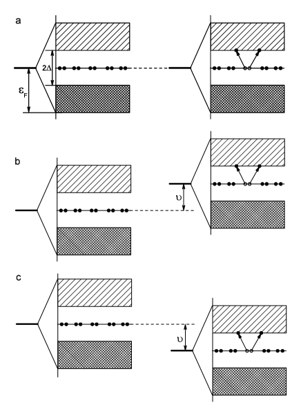
Figure 2: (a) - the process of braking of a Cooper pair in a conduction band. To break the pair with transfer of its constituents in the free quasiparticle states the energy $2|\Delta|$ is needed. (b) - the process of braking of a Cooper pair if the braking causes the increase of energy of the molecular structure by $\upsilon$ (the initial energy level shifts). (c) - it is the same, but if the braking causes the decrease of the energy.

According to BCS theory an electron-electron attraction leads to the appearance of nonzero anomalous averages $\Delta\sim\left\langle a_{-\textbf{p}\downarrow}a_{\textbf{p}\uparrow}\right\rangle$ and $\Delta^{+}\sim\left\langle a_{\textbf{p}\uparrow}^{+}a_{-\textbf{p}\downarrow}^{+}\right\rangle$, which are the order parameter (pair potential) of the superconducting state. The order parameter is determined with some self-consistency equation $\Delta=I(\Delta)$, which reflects the fact, that superconductivity is a many-particle cooperative effect. In this regime the charge is carried by pairs of electrons (current carriers are the pairs with charge $2e$). To break a pair with transfer of its constituents in free quasiparticle states the energy $2|\Delta|$ is needed. We can consider the quantity $2|\Delta|$ as a work against the effective electron-electron attraction given the fact that the quantity $\Delta$ is a collective effect. The superconducting state of a metal and the breaking of a pair are illustrated in Fig.2a.

In our model we consider a hypothetical substance, where an interaction energy between (within) structural elements of condensed matter (molecules, nanoparticles, clusters, layers, wires etc.) depends on state of Cooper pairs: if the pair is broken, then energy of the molecular system is changed by quantity $\upsilon=E_{a}-E_{b}$, where $E_{a}$ and $E_{b}$ are energies of the system after- and before the breaking of the pair accordingly. Thus to break the Cooper pair we must make the work against the effective electron-electron attraction and must change the energy of the structural elements:

$$2|\Delta|\longrightarrow 2|\Delta|+\upsilon>0.$$ (2)

We will call the parameter $\upsilon$ as the external pair potential, since it is imposed on the electron subsystem by the structural elements of a substance, unlike the pair potential $\Delta$, which is result of electron-electron interaction and determined with the self-consistency equation $\Delta=I(\Delta)$. The parameter $\upsilon$ can be either $\upsilon>0$ or $\upsilon<0$ and in the simplest case it is not function of the energy gap $|\Delta|$, $\upsilon=0$ is a trivial case corresponding to BCS theory. Moreover we suppose that $\upsilon$ does not depend on temperature essentially like parameters of electron-phonon interaction. The condition $2|\Delta|+\upsilon>0$ ensures stability of the Cooper pairs (bound state of the electrons is energetically favorable), otherwise transformation (2) has no sense and such superconducting state cannot exist. If $\upsilon<0$ then the breaking of a Cooper pair lowers energy of the molecular structure (or creation of the pair raises the energy). In this case the pairs become less stable. If $\upsilon>0$ then the breaking of the pair increases the energy (or creation of the pair lowers the energy). In this case the pairs become more stable. A possible variant of breaking of a Cooper pair in these cases is illustrated in Fig.2b and Fig.2c.

Without going into the details of interaction of the structural elements we can write an effective Hamiltonian which takes into account the effect of the structure on Cooper pairs as some effective external field, like the BCS Hamiltonian is an effective Hamiltonian describing a system of interacting electrons independently of nature of this interaction. The order parameter $\Delta$ is a complex quantity $|\Delta|e^{i\phi}$, where $\phi$ is a phase, and it is the result of a many-particle self-consistent coherent effect. In the same time the field $\upsilon$ is an additional parameter imposed on the electron subsystem by the structural elements. It is easy to see that the following transformations of the order parameter correspond to the transformation (2):

$$\Delta\longrightarrow\Delta+\frac{\Delta}{|\Delta|}\frac{\upsilon}{2}=\Delta\left(1+\frac{\upsilon}{2|\Delta|}\right),\quad\Delta^{+}\longrightarrow\Delta^{+}+\frac{\Delta^{+}}{|\Delta|}\frac{\upsilon}{2}=\Delta^{+}\left(1+\frac{\upsilon}{2|\Delta|}\right).$$ (3)

Really, the work to break the pair is

$$2\sqrt{\Delta\Delta^{+}\left(1+\frac{\upsilon}{2|\Delta|}\right)^{2}}=\left|2|\Delta|+\upsilon\right|.$$

However the transformations (3) correspond to the transformation (2) if $2|\Delta|+\upsilon>0$ only. If $2|\Delta|+\upsilon<0$ then the work is $-2|\Delta|+|\upsilon|$. Thus the model based on the transformations (3) can give ”parasitic” solutions where the condition (2) is not satisfied. Such solutions must be omitted.

The Hamiltonian corresponding to the transformations (3) is

$$\widehat{H} = \widehat{H}_{\texttt{BCS}}+\widehat{H}_{\upsilon}=\sum_{\textbf{k},\sigma}\varepsilon(k)a_{\textbf{k},\sigma}^{+}a_{\textbf{k},\sigma}-\frac{\lambda}{V}\sum_{\textbf{k},\textbf{p}}a_{\textbf{p}\uparrow}^{+}a_{-\textbf{p}\downarrow}^{+}a_{-\textbf{k}\downarrow}a_{\textbf{k}\uparrow}-\frac{\upsilon}{2}\sum_{\textbf{k}}\left[\frac{\Delta}{|\Delta|}a_{\textbf{k}\uparrow}^{+}a_{-\textbf{k}\downarrow}^{+}+\frac{\Delta^{+}}{|\Delta|}a_{-\textbf{k}\downarrow}a_{\textbf{k}\uparrow}\right]$$ (4)

where $\widehat{H}_{\texttt{BCS}}$ is BCS Hamiltonian: kinetic energy + pairing interaction, energy $\varepsilon(k)\approx v_{F}(|\textbf{k}|-k_{F})$ is measured from Fermi surface. Indeed, singling out anomalous averages $\left\langle a_{\textbf{p}\uparrow}^{+}a_{-\textbf{p}\downarrow}^{+}\right\rangle,\left\langle a_{-\textbf{p}\downarrow}a_{\textbf{p}\uparrow}\right\rangle$ and introducing the order parameter

$$\Delta^{+}=\frac{\lambda}{V}\sum_{\textbf{p}}\left\langle a_{\textbf{p}\uparrow}^{+}a_{-\textbf{p}\downarrow}^{+}\right\rangle,\quad\Delta=\frac{\lambda}{V}\sum_{\textbf{p}}\left\langle a_{-\textbf{p}\downarrow}a_{\textbf{p}\uparrow}\right\rangle,$$ (5)

we can rewrite the Hamiltonian in a form

$$\widehat{H}=\sum_{\textbf{k},\sigma}\varepsilon(k)a_{\textbf{k},\sigma}^{+}a_{\textbf{k},\sigma}+\sum_{\textbf{k}}\left[\Delta^{+}\left(1+\frac{\upsilon}{2|\Delta|}\right)a_{\textbf{k}\uparrow}a_{-\textbf{k}\downarrow}+\Delta\left(1+\frac{\upsilon}{2|\Delta|}\right)a_{-\textbf{k}\downarrow}^{+}a_{\textbf{k}\uparrow}^{+}\right]+\frac{1}{\lambda}V|\Delta|^{2}.$$ (6)

The combinations $a_{\textbf{k}\uparrow}^{+}a_{-\textbf{k}\downarrow}^{+}$ and $a_{-\textbf{k}\downarrow}a_{\textbf{k}\uparrow}$ are creation and annihilation operators of a Cooper pair, thus the mean field (3) acts on Cooper pairs. The order parameter is a complex quantity $\Delta=|\Delta|e^{i\phi}$. Due the multipliers $\frac{\Delta}{|\Delta|}$ and $\frac{\Delta^{+}}{|\Delta|}$ in $\widehat{H}_{\upsilon}$ the energy does not depend on the phase $\phi$ ($a\rightarrow ae^{i\phi/2},a^{+}\rightarrow a^{+}e^{-i\phi/2}\Longrightarrow\Delta\rightarrow\Delta e^{i\phi},\Delta^{+}\rightarrow\Delta^{+}e^{-i\phi}$). Thus both $\widehat{H}_{\texttt{BCS}}$ and $\widehat{H}_{\upsilon}$ are invariant under the $U(1)$ transformation. The term $\widehat{H}_{\upsilon}$ is similar to ”source term” in matt1 , where it means the injection of Cooper pairs into the system. On the other hand, $\widehat{H}_{\upsilon}$ has a form of an external field acting on a Cooper pairs only, and $\upsilon$ is energy of a Cooper pair in this field. Eigenfunctions of the operator $\widehat{H}$ may not be eigenfunctions of a particle number operator $\sum_{\textbf{k},\sigma}a_{\textbf{k},\sigma}^{+}a_{\textbf{k},\sigma}$, that reflects the presence of Cooper pairs’ condensate.

In our model we make the following assumptions. A change of the chemical potential at transition to superconducting state can be neglected, so that $\mu=\varepsilon_{F}$, because in the model we suppose $|\Delta|\ll\varepsilon_{F}$, that occurs for systems with week electron-electron attraction and high density of carriers, unlike the systems with the strong attraction and low particle density in the BEC regime, so that $|\Delta|>\varepsilon_{F},\mu<0$, where the change of the chemical potential plays important role in formation of the superconducting state lok . In addition we should notice that the coupling constant $\lambda$ is a sum of phonon term and Coulomb term: $\lambda=u_{ph}(\omega)-u_{c}$. In metals, as a rule, $u_{ph}(\omega)<u_{c}$ that corresponds to repulsive electron-electron interaction, however in such systems the pairing is possible as result of the second order processes, which lead to effective attraction regardless of the sign of interaction kirz : $\lambda=u_{ph}(\omega)-u_{c}^{*}$, where $u_{c}^{*}=u_{c}/\left(1+\nu_{F}u_{c}\ln\frac{\varepsilon_{F}}{\omega}\right)$ is a Coulomb pseudopotential. Such mechanism is not considered in our model. In the model we suppose a stronger condition $\lambda=u_{ph}(\omega)-u_{c}>0$, which can occur in nonmetallic superconductors (for example, in alkali-doped fullerides $\texttt{A}_{n}\texttt{C}_{60}$, where competition between the Jahn-Teller coupling and Hund’s coupling takes place han ; nom ).

In order to find equilibrium value of the order parameter $\Delta$ we should obtain system’s energy. Using the BCS wave function $\prod_{\textbf{k}}\left(u(k)+\textsl{v}(k)a_{\textbf{p}\uparrow}^{+}a_{-\textbf{p}\downarrow}^{+}\right)|0\rangle$, where $u^{2}(k)+\textsl{v}^{2}(k)=1$, we obtain the energy in a form:

$$W_{s}=\langle\widehat{H}\rangle=\sum_{\textbf{k}}2\varepsilon(k)\textsl{v}^{2}(k)-\frac{\lambda}{V}\sum_{\textbf{k},\textbf{p}}u(k)\textsl{v}(k)u(p)\textsl{v}(p)-\upsilon\frac{\Delta}{|\Delta|}\sum_{\textbf{k}}u(k)\textsl{v}(k),$$ (7)

where $\Delta$ can be supposed real in the absence of magnetic field and current. The first term is internal kinetic energy, the second term is energy of the electron-electron interaction, the third term is energy of Cooper pairs’ condensate in the external pair field. The functions $\textsl{v}(k)$ and $u(k)$ have to minimize the energy, that is $\frac{dW}{d\textsl{v}^{2}(k)}=0$:

$$2\varepsilon(k)-\frac{1-2\textsl{v}^{2}(k)}{u(k)\textsl{v}(k)}\left[\frac{\lambda}{V}\sum_{\textbf{p}}u(p)\textsl{v}(p)+\frac{\upsilon}{2}\frac{\Delta}{|\Delta|}\right]=0.$$ (8)

There are two different solutions of this equation, which correspond two different physical situations:

1. We can suppose

   $$\Delta=\frac{\lambda}{V}\sum_{\textbf{p}}u(p)\textsl{v}(p)+\frac{\upsilon}{2}\frac{\Delta}{|\Delta|}.$$ (9)

   Then we obtain the $u,\textsl{v}$ functions in a form

   $$\textsl{v}^{2}(k)=\frac{1}{2}\left(1-\frac{\varepsilon}{E}\right)\quad u^{2}(k)=\frac{1}{2}\left(1+\frac{\varepsilon}{E}\right)$$ (10)

   as in BCS theory with

   $$E^{2}=\varepsilon^{2}+|\Delta|^{2},\quad\textsl{v}(k)u(k)=\frac{\Delta}{2E}.$$ (11)

   From Eq.(9) we can see that if the coupling constant is $\lambda=0$ then the energy gap is nonzero $|\Delta|=\upsilon/2$ (if $\upsilon>0$) that corresponds to results obtained in works loz ; cap . Thus the operator $\widehat{H}_{\upsilon}$ describes the external source of Cooper pairs injecting the pairs into the system. In this case the operator $\widehat{H}_{\upsilon}$ can have a noninvariant form $\upsilon\sum_{\textbf{k}}\left[a_{\textbf{k}\uparrow}^{+}a_{-\textbf{k}\downarrow}^{+}+a_{-\textbf{k}\downarrow}a_{\textbf{k}\uparrow}\right]$. In a work matt1 this operator and its analogues are used to break down the initial symmetry of a noninteracting system and to produce the desired structure (superconducting, ferromagnetic, solid etc.) - quasiaverages Bogolyubov method. In the other case the operator can have a $U(1)\times U(1)$ symmetrical form $\sum_{\textbf{k}}\left[\upsilon a_{\textbf{k}\uparrow}^{+}a_{-\textbf{k}\downarrow}^{+}+\upsilon^{+}a_{-\textbf{k}\downarrow}a_{\textbf{k}\uparrow}\right]$, where $\upsilon$ is the order parameter of another superconductor, for example, the boundary (proximity) effect, when a superconductor is placed in contact with a normal metal schmidt or interband mixing of two order parameters belonging to different bands in a multi-band superconductor asker ; grig ; litak occurs.

2. On the other hand, in order to obtain the functions (10) we can suppose

   $$\Delta=\frac{\lambda}{V}\sum_{\textbf{p}}u(p)\textsl{v}(p),$$ (12)

   then

   $$E^{2}=\varepsilon^{2}+|\Delta|^{2}\left(1+\frac{\upsilon}{2|\Delta|}\right)^{2},\quad\textsl{v}(k)u(k)=\frac{\Delta\left(1+\frac{\upsilon}{2|\Delta|}\right)}{2E}.$$ (13)

   The integration domain in the self-consistency equation (12) must be cut off at some characteristic phonon energy $\hbar\omega$ ($\lambda>0$ if $|\varepsilon(k)|<\hbar\omega$, outside $\lambda=0$), then we have

   $$\Delta=g\int_{-\hbar\omega}^{\hbar\omega}d\varepsilon\frac{\Delta\left(1+\frac{\upsilon}{2|\Delta|}\right)}{2\sqrt{\varepsilon^{2}+|\Delta|^{2}\left(1+\frac{\upsilon}{2|\Delta|}\right)^{2}}}.$$ (14)

   We can see from Eq.(14), that if the coupling constant is $g\equiv\lambda\nu_{F}=0$ then $\Delta=0$. This means, that only electron-electron coupling is the cause of superconductivity but not the potential $\upsilon$. In this case the operator $\widehat{H}_{\upsilon}$ is an external field acting on the Cooper pairs only, and $\upsilon$ is energy of the pair in this field. As stated above, the potential $\upsilon$ is called as external pair potential since it is imposed on the electron subsystem by the structural elements of a substance (molecular, clusters etc. if their energy depends on state Cooper pairs), unlike the pair potential $\Delta$, which is result of electron-electron interaction and determined with the self-consistency equation. If $\upsilon=0$ we have usual self-consistency equation $\Delta=I(\Delta)$ in BCS theory. In presence of the external pair potential $\upsilon\neq 0$ the self-consistency condition has a form $\Delta=I(\Delta,\upsilon)$ - Eq(14). Thus the potential $\upsilon$ renormalizes the order parameter $\Delta$.

   It should be noticed that if we suppose $\Delta=0$, when $\upsilon\neq 0,g\neq 0$, then an uncertainty $\frac{\Delta}{|\Delta|}=\frac{0}{0}$ takes place in the self-consistency equation (14). That is, it would seem, $\Delta=0$ is not solution, unlike BCS theory. The absence of this solution is consequence of the fact that the derivative $\frac{dW}{d\Delta}$ does not exist at $\Delta=0$ because $W(\Delta\rightarrow 0)\sim|\Delta|$ and the function $|\Delta|$ is non-differentiable in this point (the derivative has a jump discontinuity), unlike BCS theory where $W(\Delta\rightarrow 0)\sim|\Delta|^{2}$. However, it should be noticed that the order parameter is a complex quantity: $\Delta=|\Delta|e^{i\phi}$. If $|\Delta|=0$ then the phase loses the sense so that $\langle e^{i\phi(\textbf{r},t)}\rangle=0$. Then we have $\frac{\Delta}{|\Delta|}=0$, hence $\Delta=0$ becomes a solution of the self-consistency equation (14) and it means normal state of a superconductor.

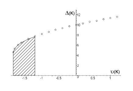
Figure 3: the energy gap $|\Delta|$ as function of the potential $\upsilon$ (in Kelvin) calculated with Eq.(14), where the parameters $g=0.25$, $\hbar\omega/k_{B}=273\texttt{K}$ have been used. If $\upsilon<0$ the critical value $\upsilon_{c}=-1.84\texttt{K}$ exists, below which the order parameter is completely suppressed. The shaded region corresponds to the metastable state, where the energy $W_{s}-W_{n}$ in Fig.(5) is positive.

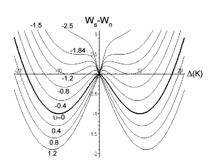
Figure 4: the energy (15) as a function of the energy gap $\Delta$ at different value of the potential $\upsilon=-2.5,-1.84,-1.4,-1.2,-0.8,-0.4,0,0.4,0.8,1.2$ in Kelvin. The bold line is the energy in BCS theory (the external pair potential is absent $\upsilon=0$). The energy $W_{s}-W_{n}$ is measured by energy of an equilibrium superconductor without the external pair potential i.e. $V\nu_{F}\frac{\Delta_{0}^{2}}{2}$, where $\Delta_{0}=10\texttt{K}$ as it can be seen from Fig.3.

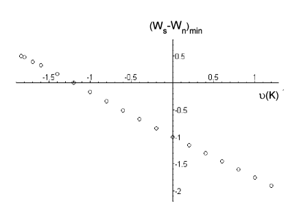
Figure 5: The minimums of the energy $W_{s}-W_{n}$ shown in Fig.4 corresponding to different values of the potential $\upsilon$. A region, where $(W_{s}-W_{n})_{min}>0$, corresponds to metastable states (it is shaded in Fig.3).

Thus a system described with the Hamiltonian (4) has the energy with two minimums (9) and (14), which correspond to two physically different situations: injection of the Cooper pairs into the system from external source - option 1, and action of the external pair potential caused by dependence of energy of the molecular structure on state of a Cooper pair - option 2. In this work we will consider the model with the external pair potential only. If $\upsilon>0$ then the pairing lowers the energy of the molecular structure, that supports superconductivity $|\Delta(\upsilon>0)|>|\Delta(\upsilon=0)|$. If $\upsilon<0$ then the pairing of electrons increases the energy of the molecular structure, that suppresses superconductivity $|\Delta(\upsilon<0)|<|\Delta(\upsilon=0)|$, moreover such a critical value of the potential $\upsilon_{c}$ exists, that if $\upsilon<\upsilon_{c}$ then Eq.(14) has not any solutions. As discussed above this region has been supposed as the normal state of a superconductor. Thus the first order phase transition (on the parameter $\upsilon$) occurs - Fig.3. From the figure we can see $2|\Delta(\upsilon)|+\upsilon>0$ for all $\upsilon\geq\upsilon_{c}$, hence the pairs are stable. In the same time Eq.(14) has solutions at $g<0,\upsilon<0$, however it can shown that in this case the condition (2) is not satisfied, that is the ”parasitic” solution occurs in this case.

Superconducting state is energetically favorable if the energy (7) of the superconducting state is less than energy of normal state i.e. $W_{s}-W_{n}<0$. The energy $W_{n}$ can be determined as $W_{n}=W_{s}(\Delta=0)$. Using Eq.(7) we have:

$$W_{s}-W_{n} = V\nu_{F}\left[\int_{-\hbar\omega}^{\hbar\omega}2\varepsilon\textsl{v}^{2}(\varepsilon)d\varepsilon-g\left(\int_{-\hbar\omega}^{\hbar\omega}\textsl{v}(\varepsilon)u(\varepsilon)d\varepsilon\right)^{2}-\upsilon\frac{\Delta}{|\Delta|}\int_{-\hbar\omega}^{\hbar\omega}\textsl{v}(\varepsilon)u(\varepsilon)d\varepsilon\right]$$ (15)

$$- V\nu_{F}\left[\int_{-\hbar\omega}^{\hbar\omega}2\varepsilon\textsl{v}_{0}^{2}(\varepsilon)d\varepsilon-g\left(\int_{-\hbar\omega}^{\hbar\omega}\textsl{v}_{0}(\varepsilon)u_{0}(\varepsilon)d\varepsilon\right)^{2}-\upsilon\int_{-\hbar\omega}^{\hbar\omega}\textsl{v}_{0}(\varepsilon)u_{0}(\varepsilon)d\varepsilon\right],$$

where

$$\textsl{v}^{2}_{0}(\varepsilon)=\frac{1}{2}\left(1-\frac{\varepsilon}{E_{0}}\right),\quad u^{2}_{0}(\varepsilon)=\frac{1}{2}\left(1+\frac{\varepsilon}{E_{0}}\right),\quad u_{0}(\varepsilon)\textsl{v}_{0}(\varepsilon)=\frac{\upsilon/2}{2E_{0}},\quad E_{0}^{2}=\varepsilon^{2}+\left(\frac{\upsilon}{2}\right)^{2}.$$ (16)

This renormalization of the normal state is a consequence of the extrapolation in the point $\Delta=0$ where the self-consistent equation (14) does not have solutions. The expressions for the energies $W_{s}$ and $W_{n}$ have not any sense in themselves, only their difference $W_{s}-W_{n}$ is a physical quantity. However for a case $\upsilon>0$ interpretation for $W_{n}$ and $E_{0}$ is possible. Let the electron-electron interaction is switched off: $g=0$. In addition it can be shown that $W_{n}<W_{n}(\upsilon=0)$. Then charge is still carried by the pairs of electrons (current carriers are the pairs) because for their breaking it must be made the work $\upsilon>0$. This means that the quasiparticle spectrum has a gap $\upsilon/2$. But this state is not superconducting because the ordering $\left\langle aa\right\rangle,\left\langle a^{+}a^{+}\right\rangle$, i.e. long-range coherence, is absent. In our opinion such state can be interpreted as state with a pseudogap. However this state principally differs from the models of pseudogap in high-$T_{c}$ superconductors dzum ; dzum1 ; dzum2 ; dzum3 ; dzum4 , where preformed uncorrelated pairs are formed due to strong electron-electron interaction, but the phase coherence is possible only at more low temperature or at more large concentration of the pairs. In our model the uncorrelated pairs are pairs in momentum space (unlike bipolarons which are pairs in real space) which exist in noninteracting Fermi system due to the external pair potential. Switching-on of the electron-electron interaction stipulates the phase coherence. The fermionic nature of the pairs for such a system is discussed in Appendix A. For the case $\upsilon<0$ such interpretation as ”pseudogap” is impossible, because at $\Delta=0$ the inequality (2) is not satisfied.

The energy (15) is shown in Fig.4. If $\upsilon=0$ we have the energy in BCS theory: the energy has symmetric minimums and a local maximum in a point $\Delta=0$. If $\upsilon>0$ then the minimums becomes deeper and are located at larger values of $|\Delta|$. If $\upsilon<0$ then the minimums becomes shallower and are located at smaller values of $|\Delta|$. At some value of $\upsilon$ the superconducting state becomes metastable, because the extremum in $\Delta=0$ becomes a local minimum with lower energy. At lager value of $|\upsilon|$ the side minimums disappear and we have only one minimum in $\Delta=0$, that means the superconducting state is suppressed. The minimums of the function $W_{s}-W_{n}$ corresponding to different quantities of the potential $\upsilon$ (that is values of the function in points determined with Eq.(14)) are shown in Fig.5. We can see the domain of metastable states, where $(W_{s}-W_{n})_{min}>0$ but Eq.(14) has solutions. The region of the solutions $\Delta(\upsilon)$ corresponding to the metastable states is shaded in Fig.3. The minimum of the energy (15) can be approximated with the expression:

$$(W_{s}-W_{n})_{min}=-V\nu_{F}\left[\frac{|\Delta|^{2}}{2}+c\cdot\upsilon|\Delta|\ln\left(\frac{2\hbar\omega}{|\Delta|}\right)\right],$$ (17)

where $c$ is a coefficient of the order of one and $|\Delta|\ll\hbar\omega$. If $\upsilon=0$ then we have the energy as in BCS theory. If $\upsilon<0$ then it can be $(W_{s}-W_{n})_{min}>0$ at $\Delta\neq 0$, that corresponds to the metastable states shown in Fig.3 and Fig.5.

III Nonzero temperatures

At nonzero temperatures thermal activated quasiparticles appears with some a distribution function $f(k)$, hence the probability that a pair $(-\textbf{k},\textbf{k})$ can be involved in formation of superconducting state is $1-2f(k)$ schmidt . Then generalizing Eq.(7) we obtain the free energy $W-TS$ in a form:

$$F_{s} = \sum_{\textbf{k}}2\varepsilon(k)\left[u^{2}(k)f(k)+\textsl{v}^{2}(k)(1-f(k))\right]-\frac{\lambda}{V}\sum_{\textbf{k},\textbf{p}}u(k)\textsl{v}(k)u(p)\textsl{v}(p)(1-2f(k))(1-2f(p))$$ (18)

$$+ 2k_{B}T\sum_{\textbf{k}}\left[f(k)\ln f(k)+(1-f(k))\ln(1-f(k))\right]-\upsilon\frac{\Delta}{|\Delta|}\sum_{\textbf{k}}u(k)\textsl{v}(k)(1-2f(k)),$$

where the first term is internal kinetic energy, the second term is energy of the electron-electron interaction, the third term is contribution of entropy, the last term is energy of Cooper pairs’ condensate in the external pair field. Minimizing the free energy $\frac{\partial F}{\partial\textsl{v}^{2}(k)}=0$ and $\frac{\partial F}{\partial f(k)}=0$ we obtain $\textsl{v}^{2}(k)=\frac{1}{2}\left(1-\varepsilon/E\right)$, $u^{2}(k)=\frac{1}{2}\left(1+\varepsilon/E\right)$ and

$$f(k)=\frac{1}{\exp\left(\frac{E}{k_{B}T}\right)+1},\quad E^{2}=\varepsilon^{2}+|\Delta|^{2}\left(1+\frac{\upsilon}{2|\Delta|}\right)^{2},$$ (19)

where

$$\Delta=\frac{\lambda}{V}\sum_{\textbf{p}}u(p)\textsl{v}(p)(1-2f(p))\Longrightarrow\Delta=g\int_{-\hbar\omega}^{\hbar\omega}d\varepsilon\frac{\Delta\left(1+\frac{\upsilon}{2|\Delta|}\right)}{2E}\tanh\left(\frac{E}{2k_{B}T}\right).$$ (20)

A solutions $\Delta(T)$ of the self-consistency equation (20) at $\upsilon<0$ are shown in Fig.6, where we can see suppression of superconductivity $|\Delta(T,\upsilon<0)|<|\Delta(T,\upsilon=0)|$ and the first order phase transition. The critical temperature (which is a function of the parameter $\upsilon$) is less than the critical temperature of the superconductor without the external pair potential $T_{c}(\upsilon<0)<T_{c}$. At $T>T_{c}(\upsilon<0)$ the equation (20) has only one solution $\Delta=0$ for reasons discussed in Section II. From Fig.6 we can see $2|\Delta(\upsilon)|+\upsilon>0$ for all temperatures $T\leq T_{c}(\upsilon<0)$, that is the work to break a Cooper pair (2) is positive, hence the pairs are stable.

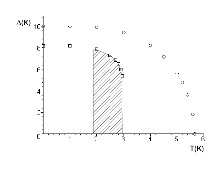
Figure 6: the energy gap as a function of temperature (in Kelvin). Circles are solutions of Eq.(20) if $\upsilon=0$ - standard result of BCS theory with the second order phase transition. Squares are solutions of Eq.(20) if $\upsilon=-1\texttt{K}<0$. The solutions demonstrate the first order phase transition. The shaded region corresponds to the metastable states, where the free energy $F_{s}-F_{n}$ is positive.

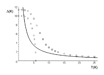
Figure 7: the energy gap as a function of temperature (in Kelvin). Circles are solutions of Eq.(20) if $\upsilon=0$ - standard result of BCS theory with the second order phase transition. Squares are solutions of Eq.(20) if $\upsilon=1\texttt{K}>0$. The solutions demonstrate, that the energy gap tends to zero asymptotically as temperature rises. Bold line is asymptotical solution (21) at large temperature.

If $\upsilon>0$ then the pairing lowers the energy of the molecular structure, that supports superconductivity $|\Delta(T,\upsilon>0)|>|\Delta(T,\upsilon=0)|$. In this case a solution of Eq.(20) is such that the order parameter is not zero at any temperature - Fig.7. At large temperature $T\gg T_{c}$, where $|\Delta(T)|\ll\upsilon$, the gap is

$$|\Delta|\approx g\int_{-\hbar\omega}^{\hbar\omega}d\varepsilon\frac{\upsilon/2}{2\sqrt{\varepsilon^{2}+(\upsilon/2)^{2}}}\tanh\left(\frac{\sqrt{\varepsilon^{2}+(\upsilon/2)^{2}}}{2k_{B}T}\right)\longrightarrow\frac{g\hbar\omega\upsilon}{4k_{B}T}.$$ (21)

Formally the critical temperature of such system is equal to infinity (in reality it limited by the melting of the substance). It should be noted that if $g=0$, then for any $\upsilon$ a superconducting state does not exist ($\Delta=0$ always). This means the electron-electron coupling is the cause of the transition to superconducting state only but not the external pair potential.

Superconducting state is energetically favorable if the free energy (18) is less than the free energy of normal state i.e $F_{s}-F_{n}<0$. The free energy $F_{n}$ can be determined as $F_{n}=F_{s}(\Delta=0)$. Then using Eq.(18) and the method of Section II - Eqs.(15,16), we can write the free energy in a form:

$$F_{s}-F_{n} = V\nu_{F}[\int_{-\hbar\omega}^{\hbar\omega}2\varepsilon\left[u^{2}f+\textsl{v}^{2}(1-f)\right]d\varepsilon-g\left(\int_{-\hbar\omega}^{\hbar\omega}\textsl{v}u(1-2f)d\varepsilon\right)^{2}$$ (22)

$$+ 2k_{B}T\int_{-\hbar\omega}^{\hbar\omega}\left[f\ln f+(1-f)\ln(1-f)\right]d\varepsilon-\upsilon\frac{\Delta}{|\Delta|}\int_{-\hbar\omega}^{\hbar\omega}\textsl{v}u(1-2f)d\varepsilon]$$

$$- V\nu_{F}[\int_{-\hbar\omega}^{\hbar\omega}2\varepsilon\left[u^{2}_{0}f_{0}+\textsl{v}^{2}_{0}(1-f_{0})\right]d\varepsilon-g\left(\int_{-\hbar\omega}^{\hbar\omega}\textsl{v}_{0}u_{0}(1-2f_{0})d\varepsilon\right)^{2}$$

$$+ 2k_{B}T\int_{-\hbar\omega}^{\hbar\omega}\left[f_{0}\ln f_{0}+(1-f_{0})\ln(1-f_{0})\right]d\varepsilon-\upsilon\int_{-\hbar\omega}^{\hbar\omega}\textsl{v}_{0}u_{0}(1-2f_{0})d\varepsilon],$$

where

$$f_{0}(\varepsilon)=\frac{1}{\exp\left(\frac{E_{0}}{k_{B}T}\right)+1},\quad E_{0}^{2}=\varepsilon^{2}+(\upsilon/2)^{2}.$$ (23)

If $\upsilon=0$ we have the free energy in BCS theory: the energy has symmetric minimums and a local maximum in a point $\Delta=0$ - Fig.9a. At $T>T_{c}$ the free energy has only one minimum in $\Delta=0$ - superconducting state is absent. The free energy (22) at different temperatures and $\upsilon=-1\texttt{K}$ is shown in Fig.8. With increasing of temperature the minimums becomes shallower and are located in smaller values of $|\Delta|$. At some temperature the superconducting states in the minimums becomes metastable, because the extremum in $\Delta=0$ becomes a minimum with lower energy. In the metastable phase the free energy $(F_{s}-F_{n})_{min}>0$ but Eq.(20) has solutions. At higher temperature these minimums disappear, and we have only one minimum in $\Delta=0$, that means the superconducting state is absent. The region of the solutions $\Delta(T)$ corresponding to the metastable states is shaded in Fig.6.

If $\upsilon>0$ then the minimums become deeper and they are located in larger values of $|\Delta|$ than in the case $\upsilon=0$ - Fig.9b. However the main difference between these cases is that the free energy at $\upsilon>0$ has absolute minimums where $(F_{s}-F_{n})_{min}<0$ at all temperatures. This means the system is in superconducting state at any temperature. The minimums of the free energy (22) at $T\rightarrow\infty$ are determined with Eq.(21).

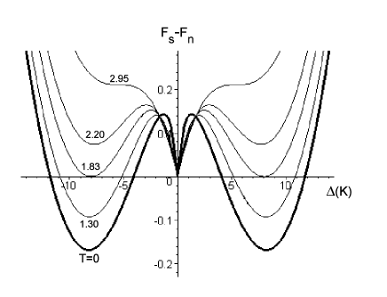
Figure 8: the free energy (22) as a function of the energy gap $\Delta$ at $\upsilon=-1\texttt{K}$ at different temperatures $T=0,1.30,1.83,2.20,2.95$ in Kelvin. The energy $F_{s}-F_{n}$ is measured by energy of an equilibrium superconductor at zero temperature without the external pair potential i.e. $V\nu_{F}\frac{\Delta_{0}^{2}}{2}$, where $\Delta_{0}=10\texttt{K}$ as it can be seen from Fig.3.

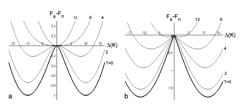
Figure 9: (a) - the free energy (22) as a function of the energy gap $\Delta$ at absence of the external pair potential $\upsilon=0$ at different temperatures $T=0,2,4,6,12$ in Kelvin. (b) - the free energy (22) at $\upsilon=1\texttt{K}$ at the same temperatures $T=0,2,4,6,12$. As in Fig.8 the energy $F_{s}-F_{n}$ is displayed as dimensionless value.

Let us consider several important limit cases. Let the external pair potential is absent $\upsilon=0$ and temperature is slightly less than the critical temperature $T\lesssim T_{c}$, hence the gap is small $\Delta\rightarrow 0$. Then we can expand the free energy (22) in powers of the order parameter:

$$F_{s}-F_{n}=V\nu_{F}\left[a(T-T_{c})|\Delta|^{2}+\frac{b}{2}|\Delta|^{4}\right],$$ (24)

where $a$ and $b$ are some coefficient. Thus we have Ginzburg-Landau expansion.

The case $\upsilon>0$ in a limit $T\rightarrow\infty$ is the most interesting. The energy gap $\Delta$ is small in this region. Then we can expand the free energy (22) in powers of $1/T$ and in powers of $|\Delta|$:

$$F_{s}-F_{n}=V\nu_{F}\left[\frac{\hbar\omega}{2k_{B}T}|\Delta|^{2}-\upsilon g\left(\frac{\hbar\omega}{2k_{B}T}\right)^{2}|\Delta|\right].$$ (25)

From condition $\frac{dF}{d|\Delta|}=0$ we obtain $|\Delta|=\frac{g\hbar\omega\upsilon}{4k_{B}T}$ that coincides with Eq.(21). It should be noted that in this limit the contribution of the kinetic energy (the first term in Eq.(18)) is proportional to $1/T^{3}$, in the same time the contribution of the entropy (the third term in Eq.(18)) is proportional to $1/T$. Thus main factor, which resists the pairing at $T\rightarrow\infty$, is the entropy, and the contribution of the kinetic energy can be omitted unlike GL expansion. Substituting the energy gap (21) in the function (25) we have a gain in the free energy for the superconducting state:

$$\left(F_{n}-F_{s}\right)_{min}=V\nu_{F}\frac{g^{2}\upsilon^{2}(\hbar\omega)^{3}}{16(k_{B}T)^{3}}=\frac{\mu_{0}H_{cm}^{2}}{2}V\Longrightarrow H_{cm}\propto\frac{\upsilon}{T^{3/2}},$$ (26)

that determines the thermodynamical magnetic field $H_{cm}$, which tends to zero asymptotically as temperature rises and is proportional to the potential $\upsilon$.

IV Free energy functional

At presence of gradient of the order parameter $\overrightarrow{\nabla}\Delta\neq 0$ (for example, when a current $\textbf{j}=2en_{s}\textbf{q}/2m$ occurs) electrons are paired with momentums $\textbf{k}+\frac{\textbf{q}}{2}$ and $-\textbf{k}+\frac{\textbf{q}}{2}$ accordingly. The nonzero momentum of the pairs causes an additional kinetic energy of the condensate, hence the expansion of superconductor’s free energy has a form schmidt :

$$F_{s}-F_{n}=-\alpha n_{s}+\frac{\beta}{2}n_{s}^{2}+n_{s}\frac{q^{2}}{4m},$$ (27)

where $n_{s}$ is the condensate’s density. In this case the density is a function of the momentum, and a critical momentum $q_{c}=\sqrt{4m\alpha}$ exists such that $n_{s}(q>q_{c})=0$. As a rule $q_{c}\propto\frac{m|\Delta|}{k_{F}}\ll k_{F}$. Thus we have to consider an operator of the kinetic energy in a form

$$\widehat{H}_{kin}=\sum_{\textbf{k}}\left[\varepsilon\left(\textbf{k}+\frac{\textbf{q}}{2}\right)a_{\textbf{k}+\frac{\textbf{q}}{2}\uparrow}^{+}a_{\textbf{k}+\frac{\textbf{q}}{2}\uparrow}+\varepsilon\left(-\textbf{k}+\frac{\textbf{q}}{2}\right)a_{-\textbf{k}+\frac{\textbf{q}}{2}\downarrow}^{+}a_{-\textbf{k}+\frac{\textbf{q}}{2}\downarrow}\right],$$ (28)

where

$$\varepsilon\left(\textbf{k}+\frac{\textbf{q}}{2}\right)\approx\varepsilon\left(k\right)+\frac{\textbf{kq}}{2m},\quad\varepsilon\left(-\textbf{k}+\frac{\textbf{q}}{2}\right)\approx\varepsilon\left(k\right)-\frac{\textbf{kq}}{2m}.$$ (29)

Using the free energy (22) with the kinetic energy calculated on the operator (28) and passing to the limit $T\rightarrow\infty,|\Delta|\ll\upsilon$ at $\upsilon>0$ we can obtain a free energy:

$$F_{s}-F_{n}=V\left[-A|\Delta|+\frac{B}{2}|\Delta|^{2}+Cq^{2}|\Delta|\right],$$ (30)

where the coefficients are

$$A=\nu_{F}g\left(\frac{\hbar\omega}{2k_{B}T}\right)^{2}\upsilon,\quad B=\nu_{F}\frac{\hbar\omega}{k_{B}T},\quad C=\nu_{F}\frac{\hbar\omega k_{F}^{2}}{144\left(k_{B}T\right)^{3}m^{2}}\upsilon.$$ (31)

Then we can obtain an equilibrium value of the gap, value of the free energy in this point and the critical momentum of the condensate accordingly:

$$\frac{\delta F}{\delta|\Delta|}=0\quad\Longrightarrow\quad|\Delta|_{min}=\frac{A}{B}\left(1-\frac{C}{A}q^{2}\right)$$ (32)

$$(F_{s}-F_{n})_{min}=-\frac{A^{2}}{2B}\left(1-\frac{C}{A}q^{2}\right)^{2}\Longrightarrow q_{c}^{2}=\frac{A}{C}$$ (33)

In the general case the vector q can run through the whole momentum space (when the pairing potential is spatially inhomogeneous $\Delta(\textbf{r})=\sum_{\textbf{q}}\Delta_{\textbf{q}}e^{i\textbf{qr}/\hbar}$), then we should sum the free energy (30) over all values of the momentum q. Moreover if the system is in a magnetic field, then the momentum q must be replaced by $\textbf{q}-2e\textbf{a}_{\textbf{q}}$, where $\textbf{a}_{\textbf{q}}$ is a Fourier component of a magnetic vector potential $\textbf{A}(\textbf{r})=\sum_{\textbf{q}}\textbf{a}_{\textbf{q}}e^{i\textbf{qr}/\hbar}$, so that $\textbf{B}=\texttt{curl}\textbf{A}$ is a magnetic induction vector. Then the free energy functional takes a form

$$F_{s}-F_{n}=V\sum_{\textbf{q}}\left[-A|\Delta_{\textbf{q}}|+\frac{B}{2}|\Delta_{\textbf{q}}|^{2}+C\left(\textbf{q}-2e\textbf{a}_{\textbf{q}}\right)^{2}|\Delta_{\textbf{q}}|+\frac{1}{2\mu_{0}\hbar^{2}}\left(q^{2}a_{\textbf{q}}^{2}-(\textbf{q}\textbf{a}_{\textbf{q}})^{2}\right)\right],$$ (34)

where the last term is energy of the magnetic field $\frac{1}{2\mu_{0}}\left(\texttt{curl}\textbf{A}\right)^{2}$. Minimizing the free energy functional (34) by the magnetic field $\frac{\delta F}{\delta\textbf{a}_{\textbf{q}}}=0$ we obtain a current in a form

$$\textbf{j}_{\textbf{q}}=4eC|\Delta|\textbf{q}-8e^{2}C|\Delta|\textbf{a}_{\textbf{q}},$$ (35)

where we can suppose $\Delta=\Delta_{\textbf{q}=0}=\frac{A}{B}$ in the local (London) limit. In a case of a singly connected superconductor using gauge transformations $\textbf{a}_{\textbf{q}}\rightarrow\textbf{a}_{\textbf{q}}+\textbf{q}/2e$ Eq.(35) can be reduced to the equation $\textbf{j}_{\textbf{q}}=-8e^{2}C|\Delta|\textbf{a}_{\textbf{q}}$ describing Meissner’s effect. The Londons’ equation can be written in a form $\textbf{j}_{\textbf{q}}=-\frac{e^{2}}{m}2n_{s}\textbf{a}_{\textbf{q}}$, where $n_{s}$ is a superfluid density (the density of correlated pairs). Then

$$n_{s}=\frac{\nu_{F}\hbar\omega k_{F}^{2}}{36\left(k_{B}T\right)^{3}m}\upsilon|\Delta|.$$ (36)

Thus the superfluid density is $n_{s}\propto\upsilon|\Delta|$, unlike BCS theory where $n_{s}\propto|\Delta|^{2}$. At the same time, as in BCS theory, the response of a superconductor to electromagnetic field is determined by the gap $\Delta$ which has long-range coherence. If $\Delta=0$ then the pseudogap $\upsilon/2$ cannot provide such electromagnetic response. General expression for the superfluid density is given in Appendix A. If we consider a superconductor with an inner cavity, then along a closed path lying within the superconductor around the cavity at a distance from the cavity’s surface larger than magnetic penetration depth we have $\textbf{j}_{\textbf{q}}=0\Rightarrow\textbf{q}=2e\textbf{a}_{\textbf{q}}\Rightarrow\hbar\nabla\varphi=2e\textbf{A}$. Integrating along the path we obtain magnetic flux quantization $\Phi=n\Phi_{0}$, where $\Phi_{0}=\frac{\pi\hbar}{e}$ is a magnetic flux quantum. Thus the free energy functional (34) describes basic properties of superconductivity.

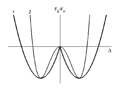
Figure 10: the schematic illustration of the free energy (30) at $\textbf{q}=0$ - line (1) and of the effective Ginzburg-Landau free energy (37) at $\textbf{q}=0,\textbf{a}_{\textbf{q}}=0$ - line (2) which have the same symmetry, the same extremes and the same values in these extremes.

Using the transformations $\Delta(\textbf{r})=\sum_{\textbf{q}}\Delta_{\textbf{q}}e^{i\textbf{qr}/\hbar},\textbf{A}(\textbf{r})=\sum_{\textbf{q}}\textbf{a}_{\textbf{q}}e^{i\textbf{qr}/\hbar}$ and the inverse transformations $\Delta_{\textbf{q}}=\frac{1}{V}\int\Delta(\textbf{r})e^{-i\textbf{qr}/\hbar}d\textbf{r},\textbf{a}_{\textbf{q}}=\frac{1}{V}\int\textbf{A}(\textbf{r})e^{-i\textbf{qr}/\hbar}d\textbf{r}$ we can write the functional Eq.(34) in real space, however the functional will have a complicated and inconvenient form due to terms $|\Delta_{\textbf{q}}|$ and $q^{2}|\Delta_{\textbf{q}}|$. Nevertheless we have seen above that the functional (34) describes basic properties of superconductivity, hence the functional can be replaced by an effective GL functional, which has the same symmetry, the same extremes and the same values in these extremes - Fig.10. The effective GL functional has a form

$$F_{s}-F_{n}=V\sum_{\textbf{q}}\left[-B|\Delta_{\textbf{q}}|^{2}+\frac{B^{3}}{2A^{2}}|\Delta_{\textbf{q}}|^{4}+\frac{BC}{A}\left(\textbf{q}-2e\textbf{a}_{\textbf{q}}\right)^{2}|\Delta_{\textbf{q}}|^{2}+\frac{1}{2\mu_{0}\hbar^{2}}\left(q^{2}a_{\textbf{q}}^{2}-(\textbf{q}\textbf{a}_{\textbf{q}})^{2}\right)\right].$$ (37)

The extremum $\Delta_{min}$, the value of the free energy $(F_{s}-F_{n})_{min}$ and the critical momentum $q_{c}$ (if there are only one q in the sum and $\textbf{a}=0$) are

$$|\Delta_{q}|_{min}=\frac{A}{B}\sqrt{1-\frac{C}{A}q^{2}},\quad(F_{s}-F_{n})_{min}=-\frac{A^{2}}{2B}\left(1-\frac{C}{A}q^{2}\right)^{2}\Longrightarrow q_{c}^{2}=\frac{A}{C}.$$ (38)

Comparing Eq.(38) with Eqs.(32,33) we can see coincidence of extremes $\Delta_{min}$ at $q=0$, coincidence of the values $(F_{s}-F_{n})_{min}$ and coincidence of the critical momentums $q_{c}$. Some different dependence $\Delta_{min}(q)$ has no basic value. The current are

$$\textbf{j}_{\textbf{q}}=4e\frac{BC}{A}|\Delta|^{2}\textbf{q}-8e^{2}\frac{BC}{A}|\Delta|^{2}\textbf{a}_{\textbf{q}}=4e\frac{AC}{B}\textbf{q}-8e^{2}\frac{AC}{B}\textbf{a}_{\textbf{q}},$$

that coincides with the current (35) in the local limit. This means that the magnetic responses will be identical.

In real space the functional (37) takes a form

$$F_{s}-F_{n}=\int\left[-B|\Delta(\textbf{r})|^{2}+\frac{B^{3}}{2A^{2}}|\Delta(\textbf{r})|^{4}+\frac{BC}{A}|\left(-i\hbar\nabla-2e\textbf{A}\right)\Delta(\textbf{r})|^{2}+\frac{(\texttt{curl}\textbf{A})^{2}}{2\mu_{0}}\right]d\textbf{r},$$ (39)

For convenience we can use a dimensionless variable $\varphi(\textbf{r})\equiv\frac{\Delta(\textbf{r})}{\Delta_{0}}=\frac{\Delta(r)}{A/B}$, then

$$F_{s}-F_{n}=\int\left[\mu_{0}H_{cm}^{2}\left(-|\varphi(\textbf{r})|^{2}+\frac{1}{2}|\varphi(\textbf{r})|^{4}+\xi^{2}\left|\left(\nabla-i\frac{2\pi}{\Phi_{0}}\textbf{A}\right)\varphi(\textbf{r})\right|^{2}\right)+\frac{(\texttt{curl}\textbf{A})^{2}}{2\mu_{0}}\right]d\textbf{r},$$ (40)

where

$$\mu_{0}H_{cm}^{2}=\frac{A^{2}}{B}\propto\frac{\upsilon^{2}}{T^{3}}$$ (41)

is thermodynamical magnetic field $H_{cm}$,

$$\xi^{2}=\hbar^{2}\frac{C}{A}\propto\frac{1}{T}$$ (42)

is a coherence length, which is determined with properties of a superconductor only (at $T\rightarrow\infty$ it does not depend on $\upsilon$). The coherence length in BCS (and in GL) theory depends on temperature as $\xi=\xi_{0}/\sqrt{1-T/T_{c}}$. That is at $T<T_{c}$ it increases as temperature rises, at $T=T_{c}$ it diverges. At $T>T_{c}$ the coherence length has physical sense of a correlation radius of fluctuations $\xi\propto(T/T_{c}-1)^{-1/2}$ which decreases as $1/\sqrt{T}$ at large $T$. The superconducting phase at $T>T_{c}$ arises fluctuationally in a form of bubble of size $\xi$ within a normal conductor, that is accompanied by an increasing of free energy (the first term in Eq.(25)). The external pair potential $\upsilon>0$ withholds the fluctuationally arisen superconducting bubbles with such $\Delta$ that the increasing in the free energy at formation of the babble is compensated by the potential $\upsilon$ (the second term in Eq.(25)). This continues until the superconducting phase does not fill the entire volume of the metal. Thus the coherence length (42) corresponds to the correlation radius of fluctuations in GL theory. It should be noted, that due to the transition to superconducting state in a region of size $\xi(T)$ a change of the free energy is

$$F_{s}-F_{n}\propto H_{cm}^{2}\xi^{3}(T)\propto\frac{\upsilon^{2}}{T^{9/2}}\ll k_{B}T,$$ (43)

that is much less a thermal energy $k_{B}T$ at $T\rightarrow\infty$. In GL theory the inequality (43) means strong fluctuations. In a case $\upsilon<0$ the situation is opposite: the normal phase arises fluctuationally in the superconductor, the external pair potential withholds the fluctuationally arisen normal bubbles until the normal phase does not fill the entire volume of the superconductor, thus superconducting phase is suppressed - Fig.(6). This is physical mechanism of the renormalization of the order parameter (14,20) by the external pair potential. Small coherence length and strong fluctuations in this model shows similarity with superfluid He II till . Apparently due to the strong fluctuations such regime of superconductivity is possible in 3D systems only. Moreover Josephson effect cannot be observed in such regime. In the same time we should notice that the fluctuations at $T\rightarrow\infty,\upsilon>0$ do not interact between themselves, since the free energy (34) does not contain terms $\propto|\Delta_{\textbf{q}}|^{4}$, unlike GL functional where the interaction of order parameter’s fluctuations plays principal role near the critical temperature: $1-T/T_{c}<Gi$ lar . Thus fluctuations in our model are fundamentally different from fluctuations within the critical domain in the standard theory.

It should be noted that phonons with lower energies than temperature of the electron gas $\hbar\omega(q)\ll k_{B}T$ are perceived by the electrons as static impurities ginz . As well known the static impurities do not influence on value of $T_{c}$ in $s$-wave superconductors (the Anderson’s theorem). However for $d$-wave pairing the nonmagnetic impurities destroy superconductivity like magnetic impurities, hence suppression of superconductivity by thermal phonons is observed in such systems and a change to the first order transition occurs gab1 ; gab2 . Thus above-described regime of superconductivity is possible in $s$-wave superconductors only.

Varying the functional (40) by $\varphi^{+}$ and A we obtain GL equations

$$\left\{\begin{array}[]{c}-\xi^{2}\left(\nabla-i\frac{2\pi}{\Phi_{0}}\textbf{A}\right)^{2}\varphi-\varphi+\varphi|\varphi|^{2}=0\\ \\ \texttt{curl}\texttt{curl}\textbf{A}=-i\frac{\Phi_{0}}{4\pi\lambda^{2}}\left(\varphi^{+}\nabla\varphi-\varphi\nabla\varphi^{+}\right)-\frac{|\varphi|^{2}}{\lambda^{2}}\textbf{A}\\ \end{array}\right\},$$ (44)

where a magnetic field penetration depth is

$$\frac{1}{\lambda^{2}}=\frac{8\pi^{2}\mu_{0}^{2}H_{cm}^{2}\xi^{2}}{\Phi_{0}^{2}}\Rightarrow\lambda\propto\frac{T^{2}}{\upsilon}.$$ (45)

The penetration depth increases with temperature, however, unlike the ordinary GL theory, it is finite quantity at all temperatures. Then GL parameter is

$$\kappa=\frac{\lambda}{\xi}\propto\frac{T^{5/2}}{\upsilon}.$$ (46)

The parameter increases with temperature unlike the ordinary GL theory, where the parameter is constant. This means that at large temperature all superconductors under the external pair potential become type II superconductors. Knowing the thermodynamical magnetic field and the magnetic penetration depth we obtain a pair-breaking current as schmidt :

$$j_{c}=\frac{2\sqrt{2}}{3\sqrt{3}}\frac{H_{cm}}{\lambda}\propto\frac{\upsilon^{2}}{T^{7/2}},$$ (47)

Besides the critical temperature an important characteristic of a superconductor are the first $H_{c1}$ and the second $H_{c2}$ critical fields. The second critical field is

$$H_{c2}=\frac{\Phi_{0}}{2\pi\mu_{0}\xi^{2}}=\sqrt{2}\kappa H_{cm}\propto T.$$ (48)

$H_{c2}$ is proportional to temperature that differs radically from GL theory, where $H_{c2}\propto 1-T/T_{c}$. In GL theory the transition to normal state in magnetic field occurs when average distance between vortexes becomes the order of the coherence length $\xi$. However in our case the length decreases with temperature $\xi\propto 1/\sqrt{T}$. This decrease compensates the rapprochement of the vortexes. The first critical field is

$$H_{c1}=\frac{H_{c2}}{2\kappa^{2}}\ln\kappa\propto\frac{\upsilon^{2}}{T^{4}}.$$ (49)

We can see the relatively strong fall with temperature, that indicates the above-mentioned tendency of transition to type II superconductivity at large temperature. The field of melting of the vortex lattice schmidt is

$$H_{m}\propto\frac{\Phi_{0}}{(k_{B}T)^{2}}\left(\frac{\Phi_{0}}{\lambda}\right)^{4}\propto\frac{\upsilon^{4}}{T^{10}}.$$ (50)

Obviously at $T\rightarrow\infty$ the field decreases with temperature faster than the first critical field $H_{m}\ll H_{c1}\ll H_{c2}$ as temperature increases. Thus in this regime the vortex lattice is not formed, that is result of above-mentioned strong fluctuations.

V Summary

In this work we have considered a hypothetical substance, where an interaction energy between (within) structural elements of condensed matter (molecules, nanoparticles, clusters, layers, wires etc.) depends on state of Cooper pairs: an additional work $\upsilon$ must be made against this interaction to break a pair. In this case the invariant under $U(1)$ transformation source of the pairs $\widehat{H}_{\upsilon}$ has to be added to BCS Hamiltonian. We have obtained a free energy for this model, which has two minimums. One of them corresponds to injection of the pairs into the system from an external source. Even if the electron-electron interaction is absent the energy gap is nonzero $|\Delta|=\upsilon/2$ (if $\upsilon>0$) that corresponds to results obtained in works loz ; cap . In another minimum (14,20) only the electron-electron coupling is the cause of superconductivity, but not the source $\widehat{H}_{\upsilon}$, however the source essentially renormalizes the order parameter: in presence of the potential $\upsilon\neq 0$ the self-consistency condition has a form $\Delta=I(\Delta,\upsilon)$. In this case we call the source as the external pair potential, since the potential is imposed on the electron subsystem by the structural elements of matter, unlike the pair potential $\Delta$, which is result of electron-electron interaction and determined with the self-consistency equation. If $\upsilon=0$ we have an usual self-consistency equation in BCS theory. If $\upsilon<0$ then the pairing of electrons increases energy of the molecular structure, that suppresses superconductivity. The phase transition conductor-superconductor becomes the first order phase transition with lower critical temperature than at $\upsilon=0$ and a region of metastable states occurs. If $\upsilon>0$ then the pairing lowers the energy of the molecular structure, that supports superconductivity. In this case at large temperatures $T\gg T_{c}$ the energy gap tends to zero asymptotically as $1/T$. Thus, formally, the critical temperature is equal to infinity, however the energy gap remains finite quantity. Hence the ratio between the gap and the critical temperature is $\Delta/T_{c}=0$ instead of finite values $\sim 1$ for all known materials. Possible realization of this model has been proposed in grig2 . It should be noted that the normal state $\Delta=0$ in this model (when $\upsilon>0$) can be considered as state with a pseudogap: since the quasiparticle spectrum $E_{0}$ has a gap $\upsilon/2$, then charge is carried by the pairs of electrons, but this state is not superconducting because the ordering $\left\langle aa\right\rangle,\left\langle a^{+}a^{+}\right\rangle$, i.e. long-range coherence, is absent. The uncorrelated pairs are pairs in momentum space (unlike bipolarons which are pairs in real space) which exist in noninteracting Fermi system due to the external pair potential. Switching-on of the electron-electron interaction stipulates the phase coherence. The superfluid density $n_{s}$ is proportional to $\upsilon|\Delta|$, unlike BCS theory where $n_{s}\propto|\Delta|^{2}$. At the same time, as in BCS theory, the response of a superconductor to electromagnetic field is determined by the gap $\Delta$ which has long-range coherence, the pseudogap $\upsilon/2$ does not give any contribution to such electromagnetic response.

For the case $\upsilon>0$ and $T\rightarrow\infty$ the effective GL free energy functional has been obtained. The functional describes a superconductor without critical temperature: the order parameter depends on temperature as $1/T$. The thermodynamical magnetic field $H_{cm}$, the first critical field $H_{c1}$ and the pair-breaking current $j_{c}$ tend to zero asymptotically as temperature increases and they are functions of the external pair potential. The magnetic penetration depth $\lambda$ increases with temperature as $T^{2}$ and it is a finite quantity at all temperatures. The coherence length $\xi$ decreases at large temperature as $1/\sqrt{T}$. The length corresponds to a size of fluctuationally arising bubbles of superconducting phase in a normal conductor (the correlation radius of fluctuations). At $T>T_{c}$ the superconducting phase arises fluctuationally in a normal conductor. The external pair potential $\upsilon>0$ withholds the fluctuationally arisen superconducting bubbles. This continues until the superconducting phase does not fill the entire volume of the metal. In this case a change of the free energy due to transition to superconducting state in the region of size $\xi(T)$ is much less a thermal energy $k_{B}T$, that means strong fluctuations. In a case $\upsilon<0$ the external pair potential withholds the fluctuationally arisen normal bubbles in a superconductor until the normal phase does not fill the entire volume of the superconductor, thus superconducting phase is suppressed. This is physical mechanism of above-mentioned renormalization of the order parameter by the external pair potential. Small coherence length and strong fluctuations in this model shows similarity with superfluid He II. Apparently due to the strong fluctuations such superconductivity is possible in 3D systems only. In the same time the fluctuations at $T\rightarrow\infty,\upsilon>0$ do not interact between themselves. Thus fluctuations in our model are fundamentally different from fluctuations within the critical domain in the standard GL theory. Moreover such superconductivity is possible in $s$-wave superconductors only due to large numbers of thermal phonons which are perceived by the electrons as static impurities.

Due to the coherence length is a decreasing function of temperature $\xi\propto 1/\sqrt{T}$ the GL parameter $\kappa=\lambda/\xi$ is an increasing function of temperature $\propto T^{5/2}$ unlike the ordinary GL theory, where the parameter is constant. Hence at large temperature all superconductors under the external pair potential become type II superconductors with the second critical field $H_{c2}$ proportional to temperature. In GL theory the transition to normal state in magnetic field occurs when average distance between vortexes becomes order of the coherence length $\xi$. However in our model the length decreases with temperature, that compensates the rapprochement of the vortexes. This result differs from results of a work grig1 , where the second critical field is infinity like the critical temperature. The free energy functional (40) has been obtained in high-temperature limit from the general expression (22). In contrast, in grig1 the free energy functional was obtained by modifying of GL expansion. Another feature of this model is that the field of melting of the vortex lattice is $H_{m}\ll H_{c1}$ at $T\rightarrow\infty$. Thus in this regime the vortex lattice is not formed, that is a result of the strong fluctuations in such a system.

Thus we propose a fundamentally different approach to the problem of increasing of critical temperature. This approach is not associated with enlargement of the coupling constant or with change of the frequency, but it allows to reformulate the problem in the sense that we change the ratio between the energy gap and the critical temperature as $\Delta/T_{c}\rightarrow 0$ at finite value of the gap. Since in this model the second critical field is an increasing function of temperature this gives opportunity to have a superconducting state at very large magnetic fields.

Appendix A Superfluid density

Hamiltonian of particles with spectrum $\varepsilon(\textbf{k})$ in the external magnetic field is

$$\widehat{H}=\int\psi^{+}(\textbf{r})\varepsilon\left(\widehat{\textbf{q}}-e\textbf{A}\right)\psi(\textbf{r})d\textbf{r},$$ (51)

where $\widehat{\textbf{q}}=-i\hbar\nabla_{\textbf{r}}$. Varying the Hamiltonian with respect to A we obtain:

$$\widehat{\textbf{j}}=e\psi^{+}(\textbf{r})\nabla_{\textbf{q}}\varepsilon\left(\textbf{q}-e\textbf{a}\right)\psi(\textbf{r}),$$ (52)

where $\textbf{a}_{\textbf{q}}=\frac{1}{V}\int\textbf{A}(\textbf{r})e^{-i\textbf{qr}/\hbar}d\textbf{r}$. Let us leave a linear relative to a term:

$$\widehat{\textbf{j}}=e\psi^{+}(\textbf{r})\nabla_{\textbf{q}}\varepsilon(\textbf{q})\psi(\textbf{r})-e^{2}\psi^{+}(\textbf{r})\nabla_{\textbf{q}}\left[(\textbf{a}\nabla_{\textbf{q}})\varepsilon(\textbf{q})\right]\psi(\textbf{r}).$$ (53)

Here the first term is a paramagnetic part and the second term is diamagnetic part of the current. Then connection between current and magnetic field takes a form:

$$\textbf{j}=Q(\textbf{q})\textbf{a}$$ (54)

where $Q(\textbf{q})=Q(0)+c\textbf{q}^{2}+\ldots$. For normal metal $Q(0)=0$, that is the diamagnetic part is exactly compensated by the paramagnetic part (Ward’s identity). In a superconductor this identity is violated:

$$Q(0)=\frac{e^{2}}{m}2n_{s},$$ (55)

where $n_{s}$ is the superfluid density - number of correlated pairs. Following levit ; sad we write the superfluid density in a form:

$$2n_{s}=n_{0}k_{B}T\sum_{n}\int_{-\infty}^{+\infty}\left[\frac{\varepsilon^{2}-\omega_{n}^{2}}{\left(\varepsilon^{2}+\omega_{n}^{2}\right)^{2}}-\frac{\varepsilon^{2}-\omega_{n}^{2}+|\Delta|^{2}}{\left(\varepsilon^{2}+\omega_{n}^{2}+|\Delta|^{2}\right)^{2}}\right]d\varepsilon=n_{0}k_{B}T\sum_{n}\frac{\pi|\Delta|^{2}}{\left(\omega_{n}^{2}+|\Delta|^{2}\right)^{3/2}},$$ (56)

where $n_{0}=\frac{p_{F}^{3}}{3\pi^{2}\hbar^{3}}=\frac{1}{3\pi^{2}}\left(\frac{2m\varepsilon_{F}}{\hbar^{2}}\right)^{3/2}$ is a total density of conduction electron, $\omega_{n}=\pi k_{B}T(2n+1)$. The first term in the square brackets corresponds to the normal state of metal only, it compensates contribution of normal electrons in the second term. For case $T=0$ the superfluid density is equal to half of the total electron density $n_{s}=n_{0}/2$ as it must be in a translationally invariant system. For case $T\rightarrow T_{c}$, where $\Delta\rightarrow 0$, we have

$$n_{s}=n_{0}\frac{7|\Delta|^{2}}{8\pi^{2}(k_{B}T_{c})^{2}}=n_{0}\left(1-\frac{T}{T_{c}}\right).$$ (57)

Thus at $T\rightarrow T_{c}$ the superfluid density decreases to zero.

For the BCS theory with the external pair potential we must take into account that the spectrum of quasiparticles is $E^{2}=\varepsilon^{2}+|\Delta|^{2}\left(1+\frac{\upsilon}{2|\Delta|}\right)^{2}$, hence the spectrum in the normal state is $E_{0}^{2}=\varepsilon^{2}+\left(\frac{\upsilon}{2}\right)^{2}$ (state with ”pseudogap”). Then the superfluid density is

$$2n_{s} = n_{0}k_{B}T\sum_{n}\int_{-\infty}^{+\infty}\left[\frac{E_{0}^{2}-\omega_{n}^{2}}{\left(E_{0}^{2}+\omega_{n}^{2}\right)^{2}}-\frac{E^{2}-\omega_{n}^{2}}{\left(E^{2}+\omega_{n}^{2}\right)^{2}}\right]d\varepsilon$$ (58)

$$= n_{0}k_{B}T\left[\sum_{n}\frac{\pi\left(|\Delta|^{2}+|\Delta|\upsilon+\left(\frac{\upsilon}{2}\right)^{2}\right)}{\left(\omega_{n}^{2}+\left(|\Delta|^{2}+|\Delta|\upsilon+\left(\frac{\upsilon}{2}\right)^{2}\right)\right)^{3/2}}-\sum_{n}\frac{\pi\left(\frac{\upsilon}{2}\right)^{2}}{\left(\omega_{n}^{2}+\left(\frac{\upsilon}{2}\right)^{2}\right)^{3/2}}\right],$$

Analogously to the previous case we have $n_{s}=n_{0}/2$ for the case $T=0$. For the case $T\rightarrow\infty$, where $\Delta\rightarrow 0$, we have

$$n_{s}=n_{0}\frac{7\upsilon|\Delta|}{8\pi^{2}(k_{B}T)^{2}},$$ (59)

that is in qualitative agreement with (36): the superfluid density is proportional to $\upsilon|\Delta|$, unlike BCS theory where $n_{s}\propto|\Delta|^{2}$. At the same time, as in BCS theory, the response of a superconductor to electromagnetic field is determined by the gap $\Delta$ which has long-range coherence. If $\Delta=0$ then the pseudogap $\upsilon/2$ cannot provide such electromagnetic response.

In Section II we could see that the normal state is a state with a pseudogap: if the ordering $\Delta\propto\left\langle aa\right\rangle,\Delta^{+}\propto\left\langle a^{+}a^{+}\right\rangle$, i.e. long-range coherence, is absent, then the quasiparticle spectrum has a gap $\upsilon/2$. This means that charge is still carried by the pairs of electrons but the pairs are not correlated. By analogy with Eqs.(56,58) the total density of pairs $n_{p}$ (correlated + uncorrelated pairs) can be found as

$$2n_{p} = n_{0}k_{B}T\sum_{n}\int_{-\infty}^{+\infty}\left[\frac{\varepsilon^{2}-\omega_{n}^{2}}{\left(\varepsilon^{2}+\omega_{n}^{2}\right)^{2}}-\frac{E^{2}-\omega_{n}^{2}}{\left(E^{2}+\omega_{n}^{2}\right)^{2}}\right]d\varepsilon,$$ (60)

As in the previous cases we have $n_{p}=n_{0}/2$ for case $T=0$. For case $T\rightarrow\infty$, where $\Delta\rightarrow 0$, we obtain

$$n_{p}=n_{0}\frac{7|\Delta|^{2}\left(1+\frac{\upsilon}{2|\Delta|}\right)^{2}}{8\pi^{2}(k_{B}T)^{2}}\approx n_{0}\frac{7\upsilon^{2}}{32\pi^{2}(k_{B}T)^{2}}.$$ (61)

Thus, the total density of pairs is proportional to $\upsilon^{2}$ (it is nonzero even when $\Delta=0$) and it tends to zero with increasing temperature slower than the superfluid density. However, the presence of the pseudogap raises the question about the fermionic or bosonic nature of Cooper pairs. Following dzum we suppose that if the size of a Cooper pair $a_{p}$ is much larger than the mean distance $R_{p}$ between the Cooper pairs then the bosonization of such Cooper pairs cannot be realized due to their strong overlapping. Thus for fermionic nature of the pair it should be $a_{p}/R_{p}>1$. Using the uncertainty principle, the size of the polaronic Cooper pairs is defined as $a_{p}(T)=\left(\hbar/2|\widetilde{\Delta}|\right)\sqrt{\varepsilon_{F}/2m}$, where $|\widetilde{\Delta}|$ is the energy gap (in our case $|\Delta|+\upsilon/2$). The size is compared with $R_{p}=(3/4\pi n_{p})^{1/3}$, where $n_{p}$ is the density of the pairs (60,61). Then for zero temperature we have $a_{p}/R_{p}\sim\varepsilon_{F}/\upsilon\gg 1$. For the case $T\rightarrow\infty$ we obtain the condition for bosonization of Cooper pairs in a form $k_{B}T>\varepsilon_{F}^{3/2}/\upsilon^{1/2}$. For evaluation let us consider a reasonable value $\upsilon\sim 10\texttt{K}$ (usual bound energy of the pairs) and $\varepsilon_{F}\sim 0.2\texttt{eV}$ (superconductors with low density of carriers, for example alkali-doped fullerides), then we have $T>10^{4}\texttt{K}$ that far exceeds the melting point of the medium. In metals this temperature is even higher. Hence the Cooper pairs have fermionic nature. Therefore the superconducting properties (critical temperature $T_{c}$ and critical magnetic fields $H_{c1}$, $H_{c2}$) can be described by the generalized BCS theory.

- (1) Gerald D. Mahan, Many-particle physics (Physics of Solids and Liquids), edition, Plenum Publ. Corp., 2000.
- (2) V.L. Ginzburg, D.A. Kirzhnits, High-temperature superconductivity, Consultants Bureau, New York and London, 1982.
- (3) V.V. Schmidt, Introduction in physics of superconductors (in Russian), MCCME, Moscow, 2000.
- (4) Rainer Wesche, Physical Properties of High-Temperature Superconductors, John Wiley Sons Ltd, 2015, https://doi.org/10.1002/9781118696644.
- (5) I.N. Askerzade, Physica C, 397 (2003) 99, https://doi.org/10.1016/j.physc.2003.07.003.
- (6) K. V. Grigorishin, Phys. Lett. A 380 (2016) 1781, https://doi.org/10.1016/j.physleta.2016.03.023.
- (7) G. Litak, T. Örd, K. Rägo and A. Vargunin, Acta Phys. Pol. A 121 (2012) 747, https://doi.org/10.12693/APhysPolA.121.747.
- (8) D.K. Efimkin, Yu.E. Lozovik, A.A. Sokolik, Phys. Rev. B 86 (2012) 115436, https://doi.org/10.1103/PhysRevB.86.115436.
- (9) S. Doniach, M. Inui, Phys. Rev. B 41 (1990) 6668, https://doi.org/10.1103/PhysRevB.41.6668.
- (10) S. Dzhumanov, E.X. Karimboev, Sh.S. Djumanov, Phys. Lett. A 380 (2016) 2173, https://doi.org/10.1016/j.physleta.2016.04.038.
- (11) A. Tagliavini, M. Capone, A. Toschi, Phys. Rev. B 94 (2016) 155114, https://doi.org/10.1103/PhysRevB.94.155114.
- (12) K.V. Grigorishin, B.I. Lev, Low Temperature Physics/Fizika Nizkikh Temperatur 41 (2015) 375, https://doi.org/10.1063/1.4919375.
- (13) R. D. Mattuk, B. Johansson, Advances in Physics 17 (1968) 509, http://dx.doi.org/10.1080/00018736800101356.
- (14) Reiner M. Dreizler, Eberhard K.U. Gross, Density Functional Theory: An Approach to the Quantum Many-Body Problem, Springer, 1990.
- (15) V.M.Loktev, S.G. Sharapov, Cond. Matter Physics (Lviv) No.11 (1997) 131, http://dx.doi.org/10.5488/CMP.11.131.
- (16) D.A. Kirzhnits, JETP Lett. 9 (1969) 360.
- (17) J.E. Han, O. Gunnarsson, Physica B 292 (2000) 196, https://doi.org/10.1016/S0921-4526(00)00482-8.
- (18) Y. Nomura, S. Sakai, M. Capone, R. Arita, J. Phys.: Condens. Matter 28 (2016) 153001, https://doi.org/10.1088/0953-8984/28/15/153001.
- (19) S. Dzhumanov, P.K. Khabibullayev, Pramana - J. Phys. 45 (1995) 385, https://doi.org/10.1007/BF02875175
- (20) S. Dzhumanov, Physica C 235-240 (1994) 2269, https://doi.org/10.1016/0921-4534(94)92356-6.
- (21) S. Dzhumanov, A. Baratov, S. Abboudy, Phys. Rev. B 54 (1996) 13121, https://doi.org/10.1103/PhysRevB.54.13121.
- (22) Dzhumanov Safarali, Theory of Conventional and Unconventional Superconductivity in the High-Tc Cuprates and Other Systems, Nova Science Publishers, 2013.
- (23) D.R. Tilley, J Tilley, Superfluidity and Superconductivity, Van Nostrand Reinhold Company, 1974.
- (24) A.I. Larkin, A.A.Varlamov, Fluctuation Phenomena in Superconductors, Springer, 2008, https://doi.org/10.1007/978-3-540-73253-2.
- (25) A.M. Gabovich, A.I. Voitenko, Phys. Lett. A 190 (1994) 191, https://doi.org/10.1016/0375-9601(94)90077-9.
- (26) A.M. Gabovich, A.I. Voitenko, Physica C 235-240 (1994) 2385, https://doi.org/10.1016/0921-4534(94)92413-9.
- (27) K.V. Grigorishin, arXiv:1610.08233 [cond-mat.supr-con]
- (28) L.S. Levitov, A.V. Shitov, Green’s Functions. Problems and Solutions (in Russian), Fizmatlit, Moscow, 2003.
- (29) M.V. Sadovskii, Diagrammatics: Lectures on Selected Problems in Condensed Matter Theory, World Scientific, 2006, https://doi.org/10.1142/9789812774361.