How wet should be the reaction coordinate for ligand unbinding?

Abstract

We use a recently proposed method called Spectral Gap Optimization of Order Parameters (SGOOP), (Tiwary and Berne, Proc. Natl. Acad. Sci 2016 113, 2839 (2016)), to determine an optimal 1-dimensional reaction coordinate (RC) for the unbinding of a bucky-ball from a pocket in explicit water. This RC is estimated as a linear combination of the multiple available order parameters that collectively can be used to distinguish the various stable states relevant for unbinding. We pay special attention to determining and quantifying the degree to which water molecules should be included in the RC. Using SGOOP with under-sampled biased simulations, we predict that water plays a distinct role in the reaction coordinate for unbinding in the case when the ligand is sterically constrained to move along an axis of symmetry. This prediction is validated through extensive calculations of the unbinding times through metadynamics, and by comparison through detailed balance with unbiased molecular dynamics estimate of the binding time. However when the steric constraint is removed, we find that the role of water in the reaction coordinate diminishes. Here instead SGOOP identifies a good one-dimensional RC involving various motional degrees of freedom. a good two dimensional reaction coordinate for the system.

I Introduction

The unbinding of ligand-substrate systems is a problem of great theoretical and practical relevance. To take an example from the biological sciences, there is now an emerging view that the pharmacological efficacy of a drug depends not just on its thermodynamic affinity for the host protein, but also, and perhaps even more so, on when and how it unbinds from the protein.Copeland, Pompliano, and Meek (2006); Copeland (2015) While a variety of experimental techniques can provide unbinding rate constants, gleaning a clear molecular scale understanding from such experiments into the dynamics of unbinding is difficult, and at best indirect. This makes it in principle very attractive to use atomistic molecular dynamics (MD) simulations to study the unbinding process. However, most successful drugs unbind at timescales much longer than milliseconds.Copeland, Pompliano, and Meek (2006); Copeland (2015) Even with the fastest available supercomputers, this makes it virtually impossible to use MD simulations to obtain statistically reliable insight into unbinding dynamics.

This timescale limitation makes it crucial to complement MD with enhanced sampling techniques. These techniques accelerate the movement between metastable states separated by high ($\gg k_{B}T$) barriers, but still allow recovering the unbiased thermodynamics and kinetics. While in principle one could construct Markov State Models (MSM) Bowman et al. (2009) to study the unbinding dynamics from multiple short, unbiased simulations without any enhanced sampling, the associated high barriers typical for unbinding make this extremely difficult. As such, reported applications of MSM to such problems have been indirect, and instead of directly studying unbinding, these studiesBuch, Giorgino, and De Fabritiis (2011); Plattner and Noé (2015) have actually looked at the drug binding problem where the barriers tend to be smaller. To directly simulate the unbinding process, it thus becomes unavoidable to use enhanced sampling methods. Pan et al. (2013)

On the other hand, the use of enhanced sampling methods to study high barrier systems has its own caveats. Many such methods involve controlling the probability distribution along a low-dimensional reaction coordinate (RC), which best captures all the relevant slow degrees of freedom. Typically many such order parameters or collective variables (CVs) are available that can distinguish between various metastable states of the system at hand. For ligand unbinding these CVs could include ligand-host relative displacement, their conformations and their hydration states. However, often the fluctuations in these CVs can be coupled in a non-trivial manner, and it can be tricky to select a RC without having a prescience of the CVs whose fluctuations matter the most for driving the process of interest.

In this work we aim to answer the following question: given a certain choice of order parameters (or collective variables) for a ligand-host system, what is the optimal 1-dimensional RC for unbinding that can be expressed as a linear combination of these collective variables? We are especially interested in determining how wet this RC is. Wetness here denotes the weight ascribed to the descriptor of the solvation state of the binding site, relative to other descriptors contributing to the RC. This will indicate how important biasing water density fluctuations in the host binding pocket is to the kinetics of ligand unbinding. While it is well-known through various theoretical, simulation and experimental studies that collective water motion into/out of binding pockets is correlated with unbinding/binding respectively Pan et al. (2013); Mondal, Morrone, and Berne (2013); Mondal, Friesner, and Berne (2014); Tiwary et al. (2015a), we wish to have a quantitative measure of the utility of biasing these water fluctuations in the sampling of ligand unbinding.

Here, we investigate this question for ligand unbinding in a much studied model hydrophobic ligand-host system (Fig. 1) interacting through Lennard-Jones potential in an aqueous environment made of explicit TIP4P water molecules.Tiwary et al. (2015a); Mondal, Morrone, and Berne (2013); Jorgensen et al. (1983) Many excellent methods exist for the purpose of RC optimization Best and Hummer (2005); Coifman et al. (2005); Peters and Trout (2006); Ma and Dinner (2005); Rohrdanz et al. (2011); Pérez-Hernández et al. (2013); Ceriotti, Tribello, and Parrinello (2011); Chen, Yu, and Tuckerman (2015). However, the energy barrier for unbinding in this system as reported through previous studies is as high as 30 – 35 $k_{B}T$, making it crucial for the purpose of RC optimization to use a method that does not rely on accurate sampling of rare reactive unbinding trajectories. For this reason we use a recently proposed method SGOOP (Spectral gap optimization of order parameters) Tiwary and Berne (2016a) that enables us to determine an optimal RC through relatively short biased simulations performed using a trial RC (see Fig. 2 and Sec. II.1 for details of SGOOP).

We consider two different scenarios in this work, both of which are expected to arise in the context of ligand unbinding. In the first scenario, we sterically constrain the system so that the ligand can move only along the centro-symmetric axis $z$ (see Fig. 1). In the second, we lift this steric constraint. We find that in the presence of the steric constraint, water density fluctuations in the host cavity must be part of the optimal RC. This is in excellent agreement with previous work on this and related systems Morrone, Li, and Berne (2012); Li, Morrone, and Berne (2012); Bolhuis and Chandler (2000); Mondal, Morrone, and Berne (2013); Tiwary et al. (2015a) where for a sterically constrained set-up, there is a bimodal water distribution at a critical ligand-cavity separation, around which the unbinding pathway involves moving from dry to wet states. However we find that when the steric constraint is removed and the ligand is free to move in any direction, the role of water in the optimal RC is minimal to none. In this case water is less of a driving variable for unbinding, but more of a driven variable that follows the movement of the ligand. Here SGOOP identifies how the optimal RC is distorted from the $z-$axis (Fig. 1), which turns out to be the minimum free energy pathway for this system as reported in a previous work.Tiwary et al. (2015a)

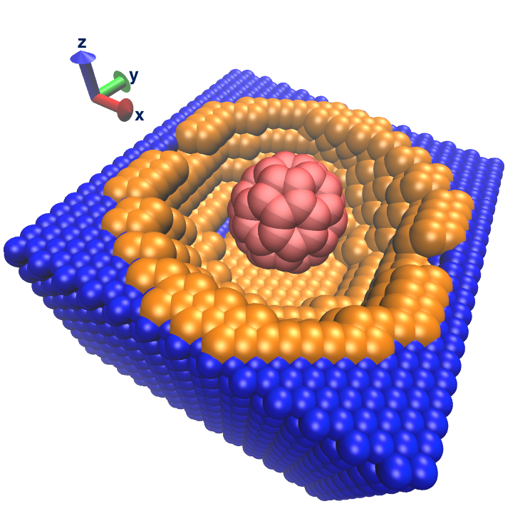
Figure 1: Cavity-ligand system in explicit water with axes marked. Red: fullerene shaped ligand atoms. Orange: cavity atoms that interact with the ligand and with water molecules. Blue: wall atoms. The water molecules are not shown for clarity. See Supplemental Information (SI) for corresponding interaction potentials.

We validate our results through extensive calculations of unbinding time statistics for the sterically constrained ligand using the infrequent metadynamics approach Tiwary and Parrinello (2013) and find that the optimal RC is indeed wet to some extent. In addition, because the analogous barrier for ligand binding is much smaller than for unbinding, we use unbiased MD estimates of the binding time and validate that detailed balance is satisfied between unbinding and binding rates. We perform the infrequent metadynamics calculations using the optimal RC as per SGOOP and two other sub-optimal RCs with no water content and more than optimal water content respectively. Our findings clearly demonstrate the improvement in the quality and accuracy of the unbinding time statistics by using the optimized RC predicted through SGOOP. With the optimized CV the unbinding time statistics give a superior agreement with the binding time statistics obtained through unbiased MD. Furthermore, it also gives a much improved Poisson fit for the cumulative distribution function of unbinding times, as quantified through the Kolmogorov-Smirnov test proposed in Ref. Salvalaglio, Tiwary, and Parrinello, 2014. This shows that the optimized RC predicted through SGOOP indeed does a better job of capturing the slow dynamics of the system. Previous applications of SGOOP Tiwary and Berne (2016a) were restricted to using the optimized RC for faster convergence of the free energy. The results reported in this work comprise the first demonstration of improving kinetics calculations using SGOOP, and mark a step further towards systematic high-throughput studies of unbinding dynamics.

II Theory

In this section we summarize the key methods Tiwary and Berne (2016a); Tiwary and Parrinello (2013); Salvalaglio, Tiwary, and Parrinello (2014) used in this work and their underlying principles.

II.1 Spectral gap optimization of order parameters (SGOOP)

SGOOP Tiwary and Berne (2016a) is a method to optimize low-dimensional order parameters or collective variables for use in enhanced sampling biasing methods like umbrella sampling and metadynamics, when only limited prior information is known about the system (see Fig. 2 for a flowchart summarizing the key steps in SGOOP). This optimization is done from a much larger set of candidate CVs $\Psi=(\Psi_{1},\Psi_{2},...,\Psi_{d})$, which are assumed to be known a priori. SGOOP is based on the idea that the best order parameter, which we call the reaction coordinate (RC), is one with the maximum separation of timescales between visible slow and hidden fast processes. This timescale separation is calculated as the spectral gap between the slow and fast eigenvalues of the transition probability matrix on a grid along any CV Tiwary and Berne (2016a). The transition probability matrix is calculated in SGOOP using an approximate kinetic model that can be derived for example through the principle of Maximum Caliber. Tiwary and Berne (2016a); Pressé et al. (2013); Dixit et al. (2015) Let $\{\lambda\}$ denote this set of eigenvalues, with $\lambda_{0}\equiv 1>\lambda_{1}\geq\lambda_{2}...$. The spectral gap is then defined as $\lambda_{s}-\lambda_{s+1}$, where $s$ is the number of barriers apparent from the free energy estimate projected on the CV at hand, that are higher than a user-defined threshold (typically $\gtrsim k_{B}T$). In this case, assuming overdamped dynamics, the eigenvalues beyond the first $s+1$ correspond to relaxation times in each of the individual wells Coifman et al. (2008); Matkowsky and Schuss (1981); Risken (1984), which for an optimal RC should be much smaller than the escape times from the wells.

Figure 2: Flowchart summarizing the various key steps in SGOOP.Tiwary and Berne (2016a) The whole process can in principle be iterated between the second and the last steps to further improve the sampling.

The key input to SGOOP as used in this work is an estimate of the stationary probability density (or equivalently the free energy) of the system, accumulated through a biased simulation performed along a sub-optimal trial RC given by some linear or non-linear function $f_{0}(\Psi)$, where $\Psi$ denotes the larger set of candidate CVs. Any type of biased simulation could be used for this purpose, as long as it allows projecting the stationary probability density estimate on generic combinations of CVs without having to repeat the simulation. Metadynamics Tiwary and Parrinello (2014) provides this functionality in a straightforward manner and hence we use it here. Given this information we use the principle of Maximum Caliber Tiwary and Berne (2016a) to set up an unbiased master equation for the dynamics of various trial CVs $f(\Psi)$. Through a post-processing optimization procedure we then find the RC as the $f(\Psi)$ which gives the maximal spectral gap of the associated transfer matrix. We refer to Ref. Tiwary and Berne, 2016a for details of the master equation and the Maximum Caliber expression that relates the transfer matrix to stationary probabilities, and facilitates calculation of the eigenvalues and hence the spectral gap.

As described in the introduction, for the problem of ligand unbinding in this work we take this larger set of CVs to be the various components of the separation between the ligand and the host, and the solvation state of the host pocket (Fig. 1). In more complex systems, further members could be added to this set. Since counting the number of barriers in a projected free energy profile could be affected by sampling noise, we smooth the free energy by averaging over bins. To ensure that the calculated spectral gaps are robust with respect to amount of smoothening, we perform an averaged estimate of the spectral gaps using different amounts of smoothing (see SI for details).

Note that the approximate kinetic model used here in SGOOP is equivalent to the Smoluchowski equation whereby (i) the dynamics of any CV is described by a forced diffusion process (ii) the diffusion constant along this CV is independent of position. This kinetic model is used in SGOOP to improve the choice of the RC that should be biased given limited information starting with a trial RC. The calculation of rates is then done with this improved RC. It is important to note that the infrequent metadynamics method for calculating rate constants Tiwary and Parrinello (2013) does not assume Smoluchowski dynamics or constant diffusivity (see following Sec. II.2 for details).

Figure 3: (a) Spectral gap versus amount of wetness of the RC, $m_{w}$ (see Eq. 2) for the case when the ligand constrained to move along a line. The optimal RC can be clearly seen to be at $m_{w}\approx 0.075$. Three different profiles are provided, which were calculated by using starting metadynamics trajectories of different lengths as indicated in legends, performed with biasing CV $z$. The spectral gap is normalized so that its value for $m_{w}=0$ is 1. (b)-(c) are the corresponding trajectories for the distance $z$ and number of pocket waters $w$. See Sec. IIIA for precise definition of $w$. In all sub-figures here, red stars, blue diamonds and magenta circles denote results for trajectories of lengths 10 ns, 15 ns and 20 ns respectively.

Figure 4: Unbinding times for the sterically constrained ligand using different simulation protocols. In (a) the mean unbinding times as obtained through the three RCs with different water coefficients are plotted along with error bars (blue circles). Also plotted is the corresponding estimate of mean unbinding time (solid black line) with errors (dashed black line) by using principle of detailed balance with the unbiased estimate of binding time. All error bars correspond to $\pm$ standard deviation intervals. (b) to (d) give the empirical (black dashed line) and fitted (solid red line) cumulative distribution functions (CDF) for unbinding time statistics using different RCs with varying amounts of wetness $m_{w}$ (see Eq. 2). From (b) to (d) respectively, $m_{w}$ is 0, 0.075 and 0.15. Also indicated are respective p-values for fit to ideal Poisson distribution, quantified using the Kolmogorov-Smirnov test from Ref. Salvalaglio, Tiwary, and Parrinello, 2014, and mean times log(2) divided by median ratio for each case. The closer are both these values to 1, the more ideal is the Poisson distribution fit illustrating the reliability of the dynamics generated from metadynamics. As can be seen from these figures, the RC with optimal water coefficient of 0.075 as obtained from SGOOP gives the best Poisson metric as per both these criteria.

II.2 Dynamics from infrequent metadynamics

The infrequent metadynamics approachTiwary and Parrinello (2013); Salvalaglio, Tiwary, and Parrinello (2014) is a recently proposed method which has been used to obtain rate constants in various molecular systems Tiwary et al. (2015b, a). It involves time-dependent biasing of a few selected (typically one to three) order parameters or collective variables (CVs) out of the many available, in order to hasten the escape from metastable free energy basins. Valsson, Tiwary, and Parrinello (2016) By periodically adding repulsive bias (typically in the form of Gaussians) in the regions of CV space as they are visited, the system is encouraged to escape stable free energy basins where they would normally be trapped for long periods of time. The central idea in infrequent metadynamics is to deposit bias rarely enough compared to the time spent in the transition state regions so that dynamics in the saddle region is very rarely perturbed. Through this approach one then increases the likelihood of not corrupting the transition states, and preserves the sequence of transitions between stable states. The acceleration of transition rates achieved through biasing can then be calculated by appealing to generalized transition state theoryBerne, Borkovec, and Straub (1988), which yields the following simple running average for the accelerationTiwary and Parrinello (2013):

$$\alpha=\langle e^{\beta V(s,t)}\rangle_{t}$$ (1)

where $s$ is the collective variable being biased, $\beta=1/k_{B}T$ is the inverse temperature, $V(s,t)$ is the bias experienced at time $t$ and the subscript $t$ indicates averaging under the time-dependent potential. This approach is expected to work best in the diffusion controlled regime.Tiwary and Berne (2016b)

This approach requires a good and small set of slow collective variables demarcating all relevant stable states of interest. Whether this is the case or not can be verified a posteriori by checking if the cumulative distribution function for the transition times out of each stable state is PoissonianSalvalaglio, Tiwary, and Parrinello (2014). While metadynamics can still be performed with two, three, or more biasing CVs, the computational gain obtained by compressing the slow dynamics into an optimized 1-dimensional RC is immense, especially given the infrequent nature of biasing (see SI for detailed simulation parameters such as frequency of biasing used in this work). Using SGOOP (Sec. II.1) allows us to select a good 1-dimensional RC as a function of the many available choice of CVs, as we show in this work. This choice increases the probability of passing the test of Ref. Salvalaglio, Tiwary, and Parrinello, 2014 once the relatively expensive infrequent metadynamics runs are performed.

III Results and discussion

III.1 Ligand constrained to move along one direction

In the first case investigated, the system dynamics is sterically constrained so that the ligand can move only along the centro-symmetric axis $z$ (Fig. 1). This system and constraint has already been investigated in studies aimed at understanding hydrophobic interactions Morrone, Li, and Berne (2012); Li, Morrone, and Berne (2012); Bolhuis and Chandler (2000); Mondal, Morrone, and Berne (2013); Tiwary et al. (2015a). Here we consider two descriptors; the $z$-component of the ligand-cavity separation, and the number of water molecules in the host cavity, denoted $w$. The number of water molecules is computed using a sigmoidal function which makes $w$ continuous and differentiable (see SI for details including precise definition of $w$) as implemented in the enhanced sampling plugin PLUMED Tribello et al. (2014). We then seek the best 1-d RC $f$ of the following form:

$$f(z,w)=\{z+m_{w}w;\text{ }m_{w}\geq 0\}$$ (2)

Throughout this paper $m_{w}$ is a measure of the wetness of the RC, with $m_{w}=0$ corresponding to a completely dry RC, and higher values denoting increasingly wetter RCs.

We first perform a short metadynamics simulation by biasing $f_{0}=z$. This starting run is performed with frequent biasing since the objective here is to get a sense of the free energy, and not the kinetics (see SI for various biasing frequencies and other parameters). Through this we can obtain an estimate of the stationary probability density along any $f(z,w)$ by using the reweighting functionality of metadynamics Tiwary and Parrinello (2014). By using SGOOP we then get an estimate of the optimal $m_{w}\approx 0.075$ in Eq. 2 which maximizes the spectral gap. This is shown in Fig. 3(a) where an estimate of the spectral gap versus $m_{w}$ for different lengths of the starting metadynamics trajectory is provided. Other trajectories used in SGOOP shown in Fig. 3 (b-c)) are for trajectories of length 10 ns, 15 ns and 20 ns respectively. The results are extremely robust with respect to simulation time, and the spectral gaps estimated with trajectories of three different simulation times are virtually indistinguishable.

The optimal wetness of the RC in Eq. 2 given by $m_{w}\approx 0.075$ is validated by by performing extensive multiple independent unbinding simulations using infrequent metadynamics (Sec. II.2). The unbinding time is calculated as the time taken to reach $z=1.4$ nm for the first time.Tiwary et al. (2015a) We perform three independent sets of 24 simulations (totaling 72 simulations) for: (1) $m_{w}=0$, a dry RC, (2) $m_{w}=0.075$, the RC with optimal wetness found from SGOOP, and (3) $m_{w}=0.15$, the RC with more than optimal wetness. The empirical and fitted cumulative distribution functions for the unbinding time statistics using the three different RCs with varying amounts of wetness are shown in Figs. 4 (b-d), along with the respective p-values for fits to ideal Poisson distributions, quantified using the Kolmogorov-Smirnov test from Ref. Salvalaglio, Tiwary, and Parrinello, 2014, and mean times log(2) divided by median ratio for each case. An ideal fit to the Poisson distribution would result if both these numbers would be close to 1, and this would suggest that the accelerated timescales found using metadynamics are reliable. The RC with optimal water coefficient $m_{w}$ = 0.075 obtained using SGOOP gives Poisson metrics closest to 1. Fig. 4 (a) shows the mean unbinding times obtained using the three RCs with different values of the wetness parameter $m_{w}$ and these are compared with the corresponding estimate provided in the literature Mondal, Morrone, and Berne (2013) calculated from accurate free energy calculations together with the principle of detailed balance. While it must be said that the completely dry RC does a reasonable job in terms of the p-value and order of magnitude agreement with unbiased MD, it is very clear from this plot as well that the RC with optimal wetness gives the best performance as per various metrics shown in Fig. 4. Thus to summarize, the optimal RC for this case indeed has a small but distinct amount of wetness.

Figure 5: Contour plot of spectral gap versus $(m_{\rho},m_{w})$ with starting metadynamics trajectory of duration 20 ns used in SGOOP. The optimal RC can be clearly seen to be at $(m_{\rho},m_{w})\approx(0.6,0.0)$. The spectral gap is normalized so that its value for $(m_{\rho},m_{w})=(0,0)$ is 1.

III.2 Ligand free to move in any direction

In this case case, we remove the steric constraint forcing the system to move along $z$, and allow the ligand to freely to move in any direction (see Fig. 1). Because the system is axially symmetric, we consider 3 order parameters, namely the $z$-component of the ligand-cavity separation, $\rho=\sqrt{x^{2}+y^{2}}$, and the number of water molecules in the host cavity, denoted $w$. We then seek the best 1-d RC $f$ of the following form:

$$f(z,\rho,w)=\{z+m_{\rho}\rho+m_{w}w;\text{ }m_{\rho}\geq 0,m_{w}\geq 0\}$$ (3)

We first perform a short metadynamics simulation by biasing with $f_{0}=z$, a purely dry RC. As before, this starting run is performed with frequent biasing since the objective here is to get a sense of the free energy, and not the kinetics. This gives an estimate of the stationary probability density along any $f(z,\rho,w)$ by applying the reweighting functionality of metadynamics.Tiwary and Parrinello (2014) We then use SGOOP we to obtain an estimate of the optimal values as $m_{\rho}\approx 0.6$, $m_{w}\approx 0.0$ in Eq. 3. These values maximize the spectral gap.

Fig. 5 gives an estimate of the spectral gap versus $(m_{\rho},m_{w})$ based on an initial metadynamics trajectory of duration 20 ns biasing $z$. The results are again extremely robust with respect to how long the simulation was run. See the SI for related data and other simulation parameters.

As can be seen by comparing Fig. 5 to Fig. 3, the wetness of the the optimal RC in the case of unconstrained motion is close to 0. In a sense the water fluctuations in the cavity appear to be caused or driven by the unbinding, rather than being a driving variable for unbinding as it is in the constrained case. The primary reaction coordinate depends on $z$ and $\rho$, the displacement variables of the ligand with respect to the cavity. Indeed SGOOP finds $m_{\rho}\approx 0.6$, which gives the distortion of the reaction path from the $z-$axis (see Fig. 1). This is the same as the slope of the minimum free energy pathway in $(z,\rho)$ space reported in previous work Tiwary et al. (2015a).

Since the optimal wetness of the RC in this case is close to 0, we do not perform any kinetics calculations. Instead we refer to the results from Ref. Tiwary et al., 2015a, where infrequent metadynamics with a similar completely dry RC for this set-up gave very good agreement through detailed balance with unbiased MD estimate of the binding time.

IV Discussion and Conclusions

In this work we have applied the recently proposed method SGOOP Tiwary and Berne (2016a) to the problem of determining the reaction coordinate for ligand unbinding in a model system in explicit water. By using short biased metadynamics simulations performed using a sub-optimal reaction coordinate, we find that the true reaction coordinate involves water in the case when the system is sterically constrained to move along an axis of symmetry. In the case when this constraint is lifted, the role of water in the optimal RC is reduced. Our predictions of the optimal RC are validated by extensive calculations of the unbinding rate constant using metadynamics with infrequent biasing Tiwary and Parrinello (2013); Salvalaglio, Tiwary, and Parrinello (2014) with different RCs. We believe that the application of SGOOP to optimize the choice of RC for ligand unbinding, combined with the approach of Refs. Tiwary and Parrinello, 2013; Salvalaglio, Tiwary, and Parrinello, 2014, provides an important step in the quest to invent methods useful for systematic and possibly high throughput calculations of the unbinding rate constant in more complex and realistic protein-ligand systems, a quantity extremely difficult to compute without careful enhanced sampling based approaches. Tiwary et al. (2015b); Teo et al. (2016) The hope is that this approach will contribute a step toward the success of computational drug discovery programs. We also think that the current work is a demonstration of how SGOOP may be used to answer similar questions in systems other than drug unbinding where the role of water density fluctuations in driving the dynamics is believed to play a role but which is hard to quantify.

Using the model system in this work allows us to study an unbinding problem involving solvation and steric related complexities, yet where we can perform extensive simulations of the reverse binding process. Undoubtedly more realistic systems will be harder to tackle than the model system of the current work, possibly involving a much larger set of trial collective variables than the current work, and requiring more care in coming up with this trial set to begin with. As long as the system’s intrinsic dynamics displays a timescale separation between few slow and remaining fast processes, and hence possesses an associated spectral gap, we expect SGOOP to be useful in obtaining a sense of fluctuations that matter for driving the dynamics in rare event systems.

We would like to emphasize that the systems considered in this work, in spite of their model nature, are in fact quite challenging test cases. This is due to the enormous barrier height involved (around 30 – 35 $k_{B}T$), and the relative insignificance of the barrier in the dewetting related bimodal distribution (around 1 – 2 $k_{B}T$)Mondal, Morrone, and Berne (2013) relative to this barrier. As such, even the trial RC that excludes wetness entirely, considered in this work and in Ref. Tiwary et al., 2015a, does a remarkably decent job when used with metadynamics.Tiwary and Parrinello (2013); Salvalaglio, Tiwary, and Parrinello (2014) Yet SGOOP does very well in picking up signals in the right directions for improving the RC towards ideality. This demonstration makes us optimistic that in more complex systems where the barrier associated to movement of water is expected to be higher Liu et al. (2005); Shan et al. (2011); Jensen et al. (2012); Tiwary et al. (2015b), the algorithm will be even more useful. Some such studies are already underway and will be the subject of future publications.

References

- Copeland, Pompliano, and Meek (2006) R. A. Copeland, D. L. Pompliano, and T. D. Meek, Nat. Rev. Drug. Discov. 5, 730 (2006).
- Copeland (2015) R. A. Copeland, Nat. Rev. Drug. Discov. (2015).
- Bowman et al. (2009) G. R. Bowman, K. A. Beauchamp, G. Boxer, and V. S. Pande, J. Chem. Phys. 131, 124101 (2009).
- Buch, Giorgino, and De Fabritiis (2011) I. Buch, T. Giorgino, and G. De Fabritiis, Proc. Natl. Acad. Sci. 108, 10184 (2011).
- Plattner and Noé (2015) N. Plattner and F. Noé, Nat. Comm. 6 (2015).
- Pan et al. (2013) A. C. Pan, D. W. Borhani, R. O. Dror, and D. E. Shaw, Drug Discov Today 18, 667 (2013).
- Mondal, Morrone, and Berne (2013) J. Mondal, J. A. Morrone, and B. J. Berne, Proc. Natl. Acad. Sci. 110, 13277 (2013).
- Mondal, Friesner, and Berne (2014) J. Mondal, R. A. Friesner, and B. Berne, J. Chem. Theor. Comp. 10, 5696 (2014).
- Tiwary et al. (2015a) P. Tiwary, J. Mondal, J. A. Morrone, and B. J. Berne, Proc. Natl. Acad. Sci. (2015a), 10.1073/pnas.1516652112.
- Jorgensen et al. (1983) W. L. Jorgensen, J. Chandrasekhar, J. D. Madura, R. W. Impey, and M. L. Klein, J. Chem. Phys. 79, 926 (1983).
- Best and Hummer (2005) R. B. Best and G. Hummer, Proc. Natl. Acad. Sci. 102, 6732 (2005).
- Coifman et al. (2005) R. R. Coifman, S. Lafon, A. B. Lee, M. Maggioni, B. Nadler, F. Warner, and S. W. Zucker, Proc. Natl. Acad. Sci. 102, 7426 (2005).
- Peters and Trout (2006) B. Peters and B. L. Trout, J. Chem. Phys. 125, 054108 (2006).
- Ma and Dinner (2005) A. Ma and A. R. Dinner, The Journal of Physical Chemistry B 109, 6769 (2005).
- Rohrdanz et al. (2011) M. A. Rohrdanz, W. Zheng, M. Maggioni, and C. Clementi, J. Chem. Phys. 134, 124116 (2011).
- Pérez-Hernández et al. (2013) G. Pérez-Hernández, F. Paul, T. Giorgino, G. De Fabritiis, and F. Noé, J. Chem. Phys. 139, 015102 (2013).
- Ceriotti, Tribello, and Parrinello (2011) M. Ceriotti, G. A. Tribello, and M. Parrinello, Proc. Natl. Acad. Sci. 108, 13023 (2011).
- Chen, Yu, and Tuckerman (2015) M. Chen, T.-Q. Yu, and M. E. Tuckerman, Proc. Natl. Acad. Sci. 112, 3235 (2015).
- Tiwary and Berne (2016a) P. Tiwary and B. J. Berne, Proc. Natl. Acad. Sci. 113, 2839 (2016a).
- Morrone, Li, and Berne (2012) J. A. Morrone, J. Li, and B. J. Berne, The Journal of Physical Chemistry B 116, 378 (2012).
- Li, Morrone, and Berne (2012) J. Li, J. A. Morrone, and B. Berne, The Journal of Physical Chemistry B 116, 11537 (2012).
- Bolhuis and Chandler (2000) P. G. Bolhuis and D. Chandler, The Journal of Chemical Physics 113, 8154 (2000).
- Tiwary and Parrinello (2013) P. Tiwary and M. Parrinello, Phys. Rev. Lett. 111, 230602 (2013).
- Salvalaglio, Tiwary, and Parrinello (2014) M. Salvalaglio, P. Tiwary, and M. Parrinello, J. Chem. Theor. Comp. 10, 1420 (2014).
- Pressé et al. (2013) S. Pressé, K. Ghosh, J. Lee, and K. A. Dill, Rev. Mod. Phys. 85, 1115 (2013).
- Dixit et al. (2015) P. D. Dixit, A. Jain, G. Stock, and K. A. Dill, J. Chem. Theor. Comp. 11, 5464 (2015).
- Coifman et al. (2008) R. R. Coifman, I. G. Kevrekidis, S. Lafon, M. Maggioni, and B. Nadler, Mult. Mod. Sim. 7, 842 (2008).
- Matkowsky and Schuss (1981) B. Matkowsky and Z. Schuss, SIAM Journal on Applied Mathematics 40, 242 (1981).
- Risken (1984) H. Risken, Fokker-planck equation (Springer, 1984).
- Tiwary and Parrinello (2014) P. Tiwary and M. Parrinello, J. Phys. Chem. B 119, 736 (2014).
- Tiwary et al. (2015b) P. Tiwary, V. Limongelli, M. Salvalaglio, and M. Parrinello, Proc. Natl. Acad. Sci. 112, E386 (2015b).
- Valsson, Tiwary, and Parrinello (2016) O. Valsson, P. Tiwary, and M. Parrinello, Annual Review of Physical Chemistry 67 (2016).
- Berne, Borkovec, and Straub (1988) B. J. Berne, M. Borkovec, and J. E. Straub, J. Phys. Chem. 92, 3711 (1988).
- Tiwary and Berne (2016b) P. Tiwary and B. J. Berne, J. Chem. Phys. 144, 134103 (2016b).
- Tribello et al. (2014) G. A. Tribello, M. Bonomi, D. Branduardi, C. Camilloni, and G. Bussi, Comp. Phys. Comm. 185, 604 (2014).
- Teo et al. (2016) I. Teo, C. G. Mayne, K. Schulten, and T. Lelièvre, Journal of Chemical Theory and Computation (2016).
- Liu et al. (2005) P. Liu, X. Huang, R. Zhou, and B. J. Berne, Nature 437, 159 (2005).
- Shan et al. (2011) Y. Shan, E. T. Kim, M. P. Eastwood, R. O. Dror, M. A. Seeliger, and D. E. Shaw, Journal of the American Chemical Society 133, 9181 (2011).
- Jensen et al. (2012) M. Ø. Jensen, V. Jogini, D. W. Borhani, A. E. Leffler, R. O. Dror, and D. E. Shaw, Science 336, 229 (2012).