Eshelby inclusions in granular matter: theory and simulations

Abstract

We present a numerical implementation of an active inclusion in a granular material submitted to a biaxial test. We discuss the dependence of the response to this perturbation on two parameters: the intra-granular friction coefficient on one hand, the degree of the loading on the other hand. We compare the numerical results to theoretical predictions taking into account the change of volume of the inclusion as well as the anisotropy of the elastic matrix.

I Introduction

Despite decades of intensive research schofield ; nedderman ; davis ; vardoulakis , the mechanics leading to strain localization in soils are not well identified. For geo-mechanicians, strain localization is the result of mechanical instabilities nedderman ; davis ; vardoulakis . When the stress exceeds a threshold (i.e. given by Mohr-Coulomb criterium for the stress component ratio), the material fails. Before such failure, soils flow plastically schofield ; davis ; vardoulakis , but the link between this plastic flow and failure is quite unclear vardoulakis . Recent approaches to describe the rheology of granular materials propose non-local constitutive relations inspired by models coming from soft glassy materials Kamrin2012 ; Bouzid2015 and introducing a new variable to describe the local state of the material (the fluidity). The physical interpretation of this fluidity is still unclear and debated Bouzid2015

Metallic glasses are another example of materials where plastic flow occurs before strain localization. It has been suggested that for these amorphous materials Argon1979a ; Argon1979b , the macroscopic plasticity is the result of numerous elementary plastic events. An elementary event may be viewed as a small and local reorganization at the molecular scale. Such events have been found in numerical simulations  Falk1998 ; Maloney2006 ; Tanguy2006 . This description in term of elementary plastic events seems also relevant for soft glassy materials (such as dense emulsions or foams) or compressed granular materials Maloney2006 . Such elementary events have been indeed reported in some experimental studies Schall2007 ; Amon2012 ; Jensen2014 ; desmond2015 ; sentjabrskaja2015 .

A very important consequence of those elementary plastic events is that they are able to interact mechanically. Indeed, when they occur, they redistribute stress in the material Picard2004 . For an elastic material, this redistribution is long-ranged and anisotropic, so that it may trigger other rearrangements further in the material along preferential directions. This coupling between plastic events is believed to be at the origin of formation of spatial heterogeneities nicolas2014 ; puosi2015 ; lin2014 ; lin2015 (such as shear band) at the macroscopic scale.

Consequently a good understanding of the stress redistribution around a single event is needed. It is a subject that has been already deeply studied, especially numerically Kabla2003 ; Maloney2006 ; Tanguy2006 , while experimental proofs of this redistribution are scarce Schall2007 ; LeBouil2014b ; desmond2015 . Those studies show that the stress redistribution around a local event may be well described using a computation done by Eshelby Eshelby1957 where an inclusion embedded in an elastic matrix spontaneously changes shape. The analytical solutions obtained from such a calculation provide a good description of the stress field measured numerically around plastic events, i.e. a quadrupolar stress redistribution. Using this theoretical representation of plastic events as Eshelby inclusions and considering the coupling between several events, predictions of the yield strain can be obtained Dasgupta2013a ; Dasgupta2013b , as well as of the inclination of shear bands Ashwin2013 ; LeBouil2014b . Active rearrangements have also been studied numerically in order to investigate the dynamics of the response of the material to a local rearrangement Puosi2014 as well as the correlation between this elastic response and the subsequent plastic events Priezjev2015 .

It has to be noted that most of the numerical studies discussed above have been done in Lennard-Jones glasses for which a domain of truly elastic response exists. So, an elastic response of the matrix surrounding a small plastic event is not a surprise. For materials which do not behave as perfectly elastically, the pertinency of Eshelby’s calculation can be questioned. Wu et al. show that the stress relaxation in liquid at times shorter than the Maxwell relaxation time may be described accordingly to Eshelby’s stress tensors wu2015 . The fourfold pattern characteristic of Eshelby’s stress tensors has observed in recent numerical studies of granular flows at constant volume guo2014 . Also, fluctuations of strains are observed experimentally LeBouil2014b with inclinations related to the maximum of the deviatoric part of Eshelby’s stress tensors. Similar oriented patterns were observed in numerical studies of compressed granular material Kuhn1999 , although the author does not link them to the Eshelby’s tensors.

The aim of this study is to show that the stress redistribution due to a local reorganization in a granular material may be unambiguously described using the Eshelby formalism. For this, we focus on a realistic situation, where the granular material evolves at fixed pressure, allowing compaction or dilatation. We implement in a discrete element numerical model of a bidimensional frictional granular assembly an active inclusion with a new procedure very close to the spirit of the demonstration of Eshelby. We show that the observed response of the granular assembly corresponds to the one expected for an elastic material Eshelby1957 . We study specifically the role of two parameters on the response of the system: the value of the friction coefficient, which governs the prevalency of sliding contacts in the system, and the loading state of the sample, i.e. its proximity to failure.

This study is organized in the following way:

In section II we explain the mode of loading of the material, which consists in a biaxial test, and we describe the preparation of the numerical experiments. We also describe the typical response obtained during the loading of the material. In section III, we give an overview of the principle of the calculation of Eshelby and we discuss our method of generating an Eshelby-type inclusion in our simulations. In section IV, we describe the stress field observed around an active inclusion at different stages of the loading and for different values of the friction coefficient. In section V we measure the angular distribution of the anisotropic response and we present the results of the evolution of the inclination of the maximum of the stress distribution as a function of the volumetric strain. We discuss the modification of the response of the system when the amount of plasticity in the granular matrix increases, either because of decreasing friction or because the system is closer to failure.

II Geometry and preparation of the numerical experiment

In this section, we present the discrete element numerical simulations and explain the method of preparation of the samples. We consider a bidimensional sample submitted to a biaxial test. This classical configuration SoilMech consists in submitting a granular sample to well-controlled stress conditions without control of the volume. Experimentally, a uniaxial compression is exerted along one direction while a confining pressure is imposed on the lateral side of the granular sample. Those kind of tests are classically used in soil mechanics to study the strain-stress properties of granular materials SoilMech . For large enough initial volume fraction, localization of the deformation is observed above a threshold Desrues2015 , with the formation of shear bands. Concerning the volumetric strain, still for initial volume fraction larger than a critical value, some compaction is observed at the beginning of the loading, followed by dilatancy at larger strain. Those kinds of test are unusual for physicists who prefer to work at constant volume and uncontrolled pressure, in order to study the behavior of a sample at a given volume fraction Majmudar2007 . Yet, confining pressure controlled set-ups are the most natural configurations when trying to understand real life granular mechanical behavior. Because we are interested in this kind of configuration, we will give special care to local change of volume in the following. As a matter of fact dilatancy and plastic deformation are closely linked in granular materials.

In Sec. II.1 and II.2, we discuss the numerical setup and test procedure. In Sec. II.3 we describe general properties of our biaxial tests.

II.1 Numerical Setup

We perform numerical simulations of a two-dimensional biaxial test. The boundary conditions are sketched in Fig. 1. $N$ grains of total mass $M_{0}$ are confined by four perpendicular walls. The left and bottom walls are fixed and motionless. The top wall moves downward with a constant velocity. These three walls can be considered to be of infinite mass, for their positions are not modified by the forces exerted by the grains. The right wall, however, is mobile, with a mass of $M_{0}/100$. It is kept in place by a constant pressure $p_{0}$.

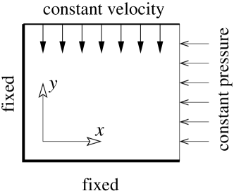
Figure 1: Set up for the numerical simulations. $N$ grains are contained within four walls: the bottom and left walls are fixed, the upper wall moves downward with constant velocity. The right wall is mobile, and subjected to a constant pressure $p_{0}$. Throughout the paper, the coordinate axes $x$ and $y$ are oriented as shown.

The grains are polydisperse disks ($r_{\mathrm{max}}/r_{\mathrm{min}}=1.5$) of uniform (two-dimensional) mass density $\rho_{0}$. The quantities $M_{0}$, $\rho_{0}$, and $p_{0}$ establish the system of units. Thus length is measured in units of $L_{0}=\sqrt{M_{0}/\rho_{0}}$, time in units of $T_{0}=\sqrt{M_{0}/p_{0}}$, and velocity in units of $V_{0}=\sqrt{p_{0}/\rho_{0}}$.

The grains interact via traditional linear, damped springs in the normal and tangential directions (normal spring constant $k_{N}=2000p_{0}$, tangential spring constant $k_{T}=k_{N}/2$). Weak linear damping is also included in these interactions. The grains also have a (microscopic) friction ratio $\mu_{m}$: the tangential force may not exceed $\mu_{m}$ times the normal force. A weak rolling resistance is added so that all vibration modes will be damped. Finally, a weak gravitational force is added to gently push “rattlers” against the granular skeleton.

All four walls are frictionless, exerting only normal forces. The mobile wall has the same stiffness as the grains, but the three walls of infinite mass are soft (spring constant $k_{\mathrm{wall}}=k_{N}/\sqrt{N}$) and dissipative. This novel boundary conditions efficiently removes vibrational energy from the system without resorting to global damping Particles2013 .

II.2 Test procedure

The simulations presented below are done with $N=256\times 256=65536$ grains. The initial state is formed by compressing a granular gas without friction (i.e. we set $\mu_{m}=0$), yielding a relatively high density. Then, at the beginning of the test, friction is turned on (i.e. we set $\mu_{m}$ to its final value), and the velocity of the top wall is set to $2\times 10^{-5}H_{0}/T_{0}$, where $H_{0}\approx 1.1L_{0}$ is the initial height of the system. We checked that decreasing further the velocity do not change the results of the simulation. As the simulation proceeds, the entire state of the system (particle positions and velocities, contact forces) are recorded at strain increments of $\Delta\varepsilon_{yy}=10^{-5}$, where the deformation $\varepsilon_{yy}$ is defined in II.3

II.3 Global properties

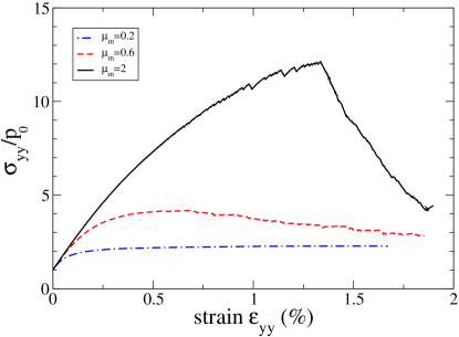
Figure 2: Stress strain curves for the simulations analyzed in this paper.

In Fig. 2, we show the stress-strain curve for the simulations studied in this paper. The stress is deduced from the force exerted by the grains on the upper (constant velocity) wall. The strain is usually deduced in simulations from the position of this wall, but that does not work in this situation due to the softness of the wall. Indeed, more than half of the apparent deformation can occur at the wall, and not within the packing. Instead, we return to the definition of strain: $\varepsilon_{yy}=\partial u_{y}/\partial y$, where $u_{y}$ is the $y$-component of the displacement of a material point relative to a reference state. We therefore calculate the displacement of each grain, and accumulate $N$ pairs $(y,u_{y})$, and then do a linear regression and take the slope of as $\Delta\varepsilon_{yy}$, the deformation from the reference state. At the beginning of the simulation, the initial condition is the reference state, but each time the deformation increases by $10^{-5}$, the reference state is updated. The total deformation, averaged over the full sample, is $\varepsilon_{yy}$ in Fig. 2 and in the rest of the paper.

Fig. 2 shows that we can control the peak stress by changing the friction ratio $\mu_{m}$. For $\mu_{m}=0.2$ and $\mu_{m}=0.6$, we obtain results similar to those obtained experimentally or in other numerical experiments. When $\mu_{m}=2$, the peak stress exceeds $10$ times the confining pressure. This quite high value do not correspond to experimental values of grain-grain friction coefficients. However, it is an interesting limit case for theoretical reasons.

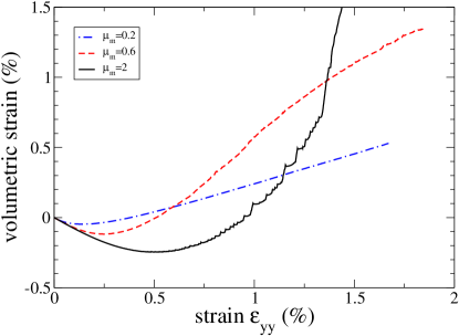
Figure 3: Volumetric strain $\varepsilon_{xx}+\varepsilon_{yy}$ for the tests studied in this paper.

In Fig. 3, we show the volumetric strain $\varepsilon_{xx}+\varepsilon_{yy}$ during the tests. (The strain component $\varepsilon_{xx}$ is determined in the same way as $\varepsilon_{yy}$ strain component.) This result is in agreement with the experimental observations in biaxial and triaxial tests: the loading curve presents a maximum and the volumetric strain first decreases before continuously increasing.

III Eshelby’s inclusion: theory and numerical implementation

In this part we present our method for implementing an active inclusion in a granular material. Active inclusions in numerical simulation have been considered recently Puosi2014 ; Priezjev2015 in two-dimensional Lennard-Jones glasses by imposing displacements on the particles forming the inclusion. This approach amounts to imposing a strain on the inclusion. Here we propose a new procedure to implement an active inclusion where a stress is imposed. We do this for two reasons. First of all, we are dealing with granular materials, where changes of volume are very important. Thus we want to leave the inclusion free to choose the volume it wants. Second, the stress we impose appears at the beginning of the Eshelby’s calculation Eshelby1957 . We will explain this more precisely below.

Eshelby gave a general method based on the linear superposition of small deformation elasticity to solve a class of problems implicating an inclusion in an elastic matrix. He also gives analytical solutions of several typical problems. In the following, we will use the solution of this problem: consider a small part of an infinite elastic matrix which we will call the inclusion. Suppose that this inclusion has a spontaneous change of shape. The Eshelby solution of interest for us gives the stress field distribution in the matrix due to that local event when the unconstrained spontaneous change of shape of the inclusion is known.

The coordinate system used in the following is given in Fig. 1. For the vector positions, we use the polar coodinates $\vec{r}=r\vec{n}=r\left(\begin{array}[]{c}\cos\theta\\ \sin\theta\end{array}\right)$. The origin is taken at the center of the inclusion. In all the considered cases, the imposed stress at the boundaries corresponds to biaxial stress-imposed configuration:

$$\mathbf{\sigma^{\infty}}=\left(\begin{array}[]{cc}\sigma^{\infty}_{xx}&0\\ 0&\sigma^{\infty}_{yy}\\ \end{array}\right)$$

with $\sigma^{\infty}_{xx}\text{ and }\sigma^{\infty}_{yy}<0$, and $\sigma^{\infty}_{xx}-\sigma^{\infty}_{yy}>0$.

In this theoretical section, we first recall the general principle of Eshelby’s calculation. In the second part, we give the general form of the analytical solution far from the inclusion. In the last part our method of generating Eshelby-type inclusion in the numerical simulation is described.

III.1 Principle of the calculation

Consider an inclusion, within an infinite elastic matrix, which undergoes a spontaneous change of shape. If it had not been inside a matrix, this change of shape would correspond to the homogeneous strain tensor $e_{ij}^{*}$. The elastic stress field associated to this strain tensor is $\sigma_{ij}^{*}=\lambda e_{kk}^{*}\delta_{ij}+2\mu e_{ij}^{*}$, $\lambda$ and $\mu$ being the Lamé coefficients Landau .

As the inclusion is in a matrix, its change of shape will interact with the elastic surrounding medium, leading to a displacement field $\tilde{u}_{i}(\vec{r})$ in the matrix, generated by the rearrangement and given in 2D by:

$$\tilde{u}_{i}(\vec{r})=\int_{\mathcal{C}}G_{ij}^{2D}(\vec{r}-\vec{r^{\prime}})\sigma_{jk}^{*}dc_{k}^{\prime}$$ (1)

where the integral covers the inclusion contour $\mathcal{C}$, $G_{ij}^{2D}(\vec{r}-\vec{r^{\prime}})$ is the bidimensional Green function giving the displacement response awaited at $\vec{r}$ from a ponctual unitary force exerted in $\vec{r^{\prime}}$ belonging to the contour on an element $dc_{k}^{\prime}$ Landau ; Eshelby1957 .

The following part discusses the far-field redistributed deviatoric stress for $e_{ij}^{*}$ coaxial with the loading $\sigma^{\infty}_{ij}$. Complete solutions (with near-field terms) of the previous equations in the case of an elliptical inclusion can be found in Ashwin2013 .

III.2 Coaxial solutions

The displacement field in the matrix far from the inclusion can be approximated by (see Appendix A):

$$\tilde{u_{i}}(\vec{r})=\frac{S}{2\pi r}\frac{\lambda+\mu}{\lambda+2\mu}e_{jk}^{*}g_{ijk}^{2D}(\vec{n})$$ (2)

where $S$ is the area of the inclusion. The function $g_{ijk}^{2D}(\vec{n})$ depends only on the direction $\vec{n}$ (see Eq. 21). The explicit determination of the solution depends on the expression of $e_{ij}^{*}$. In the present study, we restrict to the case of strain tensors characterizing the plastic rearrangement coaxial to the uniform imposed stress tensor $\mathbf{\sigma^{\infty}}$, i.e.:

$$\mathbf{e}^{*}=\left(\begin{array}[]{cc}e^{*}_{xx}&0\\ 0&e^{*}_{yy}\end{array}\right)$$ (3)

The geometry of the loading motivates this hypothesis. Furthermore, Dasgupta et al. Dasgupta2013a ; Dasgupta2013b have shown that this orientation minimizes the energy of interaction between the external strain field and the inclusion at high enough strain. The components of the strain tensor $\mathbf{\tilde{e}}$ induced by the rearrangement in the surrounding matrix can then be computed explicitly (see Appendix A).

In a biaxial experiment, the crucial quantity which characterizes the shear and which governs the response of the material is the deviatoric stress $\sigma_{xx}-\sigma_{yy}$. The significant component of the stress redistribution to determine is thus the redistributed deviatoric stress $\tilde{\sigma}_{xx}-\tilde{\sigma}_{yy}$, which will add to the imposed stress field and will thus modify locally the total deviatoric stress. Here, we obtain from (2) (see Appendix A):

$$\tilde{\sigma}_{xx}-\tilde{\sigma}_{yy}\propto\frac{S}{\pi r^{2}}\frac{\lambda+\mu}{\lambda+2\mu}f(\theta)$$ (4)

with

$$f(\theta)=-(e_{xx}^{*}+e_{yy}^{*})\cos(2\theta)-(e_{xx}^{*}-e_{yy}^{*})\cos(4\theta)$$ (5)

This function has a quadrupolar part which originates from the shear part of the strain: $(e_{xx}^{*}-e_{yy}^{*})$ and a bipolar part due to the volumetric strain $(e_{xx}^{*}+e_{yy}^{*})$. The function $f(\theta)$ is independent of the elasticity coefficients because we are in two dimensions. In three dimension the corresponding function depends on the Poisson’s ratio.

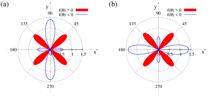
Figure 4: Polar representation of the function $f(\theta)$ (Eq. 5). (a) Contractant event: $e_{xx}^{*}=.3$ and $e_{yy}^{*}=-.7$. (b) Dilatant event: $e_{xx}^{*}=.7$ and $e_{yy}^{*}=-.3$.

Figure 4(a) (resp. (b)) shows polar representations of the function $f(\theta)$ in a contracting (resp. dilating) case. We observe a dominant quadrupolar response with an increase of the deviatoric stress along directions close to $45^{\circ}$ from the principal stresses (red curve of Fig. 4). The change of volume induces a small modification of this inclination as well as an asymmetry in the negative part of deviatoric stress redistribution (blue curves of Fig. 4). This negative contribution counteract the macroscopic loading $\sigma_{xx}^{\infty}-\sigma_{yy}^{\infty}$.

III.3 Generating numerically an Eshelby inclusion

A careful reading of Sec. III.1, especially of Eq. (1), shows that the stress redistribution due to the inclusion is obtained by integrating Green function for stress over the boundary of the inclusion. In the simulations, therefore, we will define a small inclusion, and then modify the stress at the boundary. But since the simulation is discrete, we must apply this stress in a discrete way.

We specify a perturbing stress $\bm{\sigma}^{*}$, and not a perturbing strain $\bm{e}^{*}$ because in Eshelby’s calculation, it is the stress that is propagated into the material [see Eq. (1)]. The perturbing stress is obtained from the perturbing strain, using the elastic coefficients. In our case, the elastic coefficients are not known, so that a more direct comparison can be obtained by directly imposing a stress.

Let us suppose that we want to estimate the stress in some region $\mathbb{V}$. We have Alexander98

$$\bm{\sigma}=\frac{1}{S}\sum_{\alpha\in\mathbb{A}}\mathbf{F}_{\alpha}\otimes\mathbf{r}_{\alpha},$$ (6)

where $S=|\mathbb{V}|$ is the area (in two-dimensions) of the region where we calculate the stress. The variable $\alpha$ labels the contacts and $\mathbb{A}$ is the set of contacts with at least one grain within $\mathbb{V}$. (A grain is in $\mathbb{V}$ if its center is in $\mathbb{V}$). The force between the grains is $\mathbf{F}_{\alpha}$, $\mathbf{r}_{\alpha}$ is a vector along which the force is transmitted inside $\mathbb{V}$, and $\otimes$ indicates a tensor (dyadic) product.

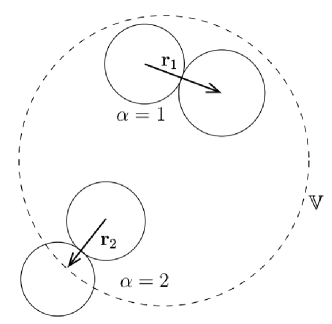
Figure 5: Two contacts inside the region $\mathbb{V}$ where the stress is being calculated. Upper contact ($\alpha=1$): both grains lie within $\mathbb{V}$, $\mathbf{r}_{1}$ is the line of centers. Lower contact ($\alpha=2$): only one grain lies within $\mathbb{V}$, $\mathbf{r}_{2}$ extends from this grain, along the line of centers, to the boundary of $\mathbb{V}$.

Some contacts in $\mathbb{A}$ have both grains in $\mathbb{V}$ while others have only one – see Fig. 5. Let $\mathbb{B}$ be the set of all contacts with two grains in $\mathbb{V}$ while $\mathbb{C}=\mathbb{A}\backslash\mathbb{B}$ is the set of all contacts with one grain in $\mathbb{V}$. The vector $\mathbf{r}_{\alpha}$ depends on whether the contact $\alpha$ is in $\mathbb{B}$ or $\mathbb{C}$. If $\alpha\in\mathbb{B}$ (both grains in $\mathbb{V}$), then $\mathbf{r}_{\alpha}=\mathbf{x}_{j_{\alpha}}-\mathbf{x}_{i_{\alpha}}$, where $i_{\alpha},j_{\alpha}$ label the two particles participating in contact $\alpha$. On the other hand, if $\alpha\in\mathbb{C}$, then $\mathbf{r}_{\alpha}={\mathbf{x}^{\circ}_{\alpha}}-\mathbf{x}_{i_{\alpha}}$, where $\mathbf{x}^{\circ}_{\alpha}$ is the point where the line of centers crosses the boundary of $\mathbb{V}$. We can therefore rewrite Eq. (6) as

$$\bm{\sigma}=\frac{1}{S}\sum_{\alpha\in\mathbb{B}}\mathbf{F}_{\alpha}\otimes(\mathbf{x}_{j_{\alpha}}-\mathbf{x}_{i_{\alpha}})+\frac{1}{S}\sum_{\alpha\in\mathbb{C}}\mathbf{F}_{\alpha}\otimes(\mathbf{x}^{\circ}_{\alpha}-\mathbf{x}_{i_{\alpha}}).$$ (7)

Instead of a sum over contacts, we can now write the stress as a sum over grains. We must define two new sets: let $\mathbb{G}$ be the set of all grains whose centers are in $\mathbb{V}$, and let $\mathbb{A}_{i}$ be the set of all contacts involving grain $i$. Then we have

$$\bm{\sigma}=\frac{1}{S}\sum_{i\in\mathbb{G}}\left[\sum_{\alpha\in\mathbb{A}_{i}}\chi_{i\alpha}\mathbf{F}_{\alpha}\right]\otimes\mathbf{x}_{i}+\frac{1}{S}\sum_{\alpha\in\mathbb{C}}\mathbf{F}_{\alpha}\otimes\mathbf{x}^{\circ}_{\alpha}.$$ (8)

Here, $\chi_{i\alpha}=\pm 1$, depending on whether we have $i=i_{\alpha}$ or $i=j_{\alpha}$.

Now the sum in brackets in Eq. (8) vanishes when the grains are in equilibrium, for it is simply the sum of forces exerted on grain $i$. The first term of Eq. (8) thus vanishes, leaving only those contacts that cross the boundary:

$$\bm{\sigma}=\frac{1}{S}\sum_{\alpha\in\mathbb{C}}\mathbf{F}_{\alpha}\otimes\mathbf{x}^{\circ}_{\alpha}.$$ (9)

This equation tells us that the stress inside a region is determined just by the contacts that span the boundary.

Up to now, we have been considering these equations from a diagnostic point of view, that is, the contact forces and grain positions are extracted from numerical data, and then the stress tensor is calculated in view of passing over to a continuum description. Now we will take a different perspective: the stress tensor on the left hand side is a perturbing stress that we want to apply inside $\mathbb{V}$, while the forces on the right hand side are modifications of the contact forces that we will introduce in order to apply that stress. Accordingly, we now write

$$\bm{\sigma}^{*}=\frac{1}{S}\sum_{\alpha\in\mathbb{C}}\mathbf{F}^{*}_{\alpha}\otimes\mathbf{x}^{\circ}_{\alpha}.$$ (10)

where we have written a star next to the stress tensor [as in Eq. (1)], and next to the forces, to indicate this new perspective.

Our method for generating an active inclusion consists of first choosing the stress $\bm{\sigma}^{*}$, and then choosing forces $\mathbf{F}^{*}_{\alpha}$ so that Eq. (10) holds. The forces can then be added directly to the simuation.

We emphasize that our method begins with $\bm{\sigma}^{*}$, that appears in Eq. (1), at the beginning of Eshelby’s calcution. The alternative of imposing displacements Puosi2014 ; Priezjev2015 corresponds to imposing $\tilde{u}_{i}$ inside the inclusion. But Eshelby’s calculation does not begin with $\tilde{u}_{i}$, but rather with $\bm{\sigma}^{*}$ (or $\bm{e}^{*}$ if the elastic moduli are known).

Now let us return to the description of our method and consider the special case where $\mathbb{V}$ is a circle of radius $R$ ($S=\pi R^{2}$), as shown in Fig. 5. The points $\mathbf{x}_{\alpha}^{\circ}$ are all located on the circle. Placing the origin at the center of the circle, their coordinates can be written in terms of the $R$ and the unit vector $\mathbf{n}_{\alpha}=\begin{pmatrix}\cos\theta_{\alpha}\\ \sin\theta_{\alpha}\end{pmatrix}$. We have

$$\bm{\sigma}^{*}=\frac{1}{\pi R}\sum_{\alpha\in\mathbb{C}}\mathbf{F}^{*}_{\alpha}\otimes\mathbf{n}_{\alpha}$$ (11)

When we specify $\bm{\sigma}^{*}$, Eq. (11) contains four equations and $2|\mathbb{C}|$ unknowns because each $\mathbf{F}^{*}_{\alpha}$ is unknown and contains two components. The volume $\mathbb{V}$ is chosen to approximate the circular inclusion of the Eshelby calculation, and therefore must be larger than the grain size, leading to $|\mathbb{C}|\gg 1$. Thus the system (11) is always under-determined. To add extra conditions, we minimize $\sum_{\alpha\in\mathbb{C}}|\mathbf{F}^{*}_{\alpha}|^{2}$. The meaning of this condition is that we look for the microscopic force distribution obeying Eq. (11) which disturbs the medium as little as possible. We therefore use Lagrange multipliers to minimize $\sum_{\alpha\in\mathbb{C}}|\mathbf{F}^{*}_{\alpha}|^{2}$ subject to the condition in Eq. (11). We thus minimize

$$\mathcal{L}=\sum_{\alpha\in\mathbb{C}}|\mathbf{F}^{*}_{\alpha}|^{2}-\bm{\lambda:}\left[\pi R\bm{\sigma}^{*}-\sum_{\alpha\in\mathbb{C}}\mathbf{F}^{*}_{\alpha}\otimes\mathbf{n}_{\alpha}\right].$$ (12)

Here, $\bm{\lambda}$ is matrix of Lagrange multipliers, and the two points signify a total contraction between two matrices ($\mathbf{A:B}=A_{ij}B_{ij}$).

Differentiating Eq. (12) by the forces, we get

$$\mathbf{F}^{*}_{\alpha}=\frac{1}{2}\bm{\lambda}\mathbf{n}_{\alpha}.$$ (13)

The Lagrange multipliers can be found by putting the forces in to the conditions Eq. (10):

$$2\pi r\bm{\sigma}^{*}=\bm{\lambda}\begin{pmatrix}A&C\\ C&B\end{pmatrix}.$$ (14)

where $A=\sum_{\alpha\in\mathbb{C}}\cos^{2}\theta_{\alpha}$, $B=\sum_{\alpha\in\mathbb{C}}\sin^{2}\theta_{\alpha}$, $C=\sum_{\alpha\in\mathbb{C}}\cos\theta_{\alpha}\sin\theta_{\alpha}$.

Before passing on to the results, we remark that a pair of grains can be considered as a contact in the set $\mathbb{C}$ even if the two grains are not touching. In that case the contact force vanishes, but that contact can be used to apply the perturbing stress.

IV Results of the numerical experiment

In this section we study the response of the granular material to a provoked Eshelby inclusion.

IV.1 Generation of a response to an Eshelby inclusion

We compute the response to an Eshelby inclusion in the following way. We first perform a compression of the granular material as described in II.1 up to a given deformation. We then identify a small circle region of radius $R=L_{0}/80$ (approximately 6 grain radii) at the center of the sample. This small circle is the region $\mathbb{V}$ discussed above. For a region two times larger, the results presented below are unchanged. We also tested $R=L_{0}/160$, and the main effect seems to be to rotate the far-field response by of order $10^{\circ}$. If $R$ is reduced another factor of two, there are not enough contacts to apply the perturbuation.

We then perform two simulations. In the first simulation, we simply continue the biaxial test without adding the perturbing force. The second simulation has exactly the same duration as the first, except that the perturbing forces are gradually “turned on” over a time long enough to avoid the generation of shock waves.

Then the stress $\bm{\sigma}_{i}$ on each grain $i$ is calculated as a sum over that grain’s contacts. Using the notation of the previous section,

$$\bm{\sigma}_{i}=\frac{1}{\pi r_{i}^{2}}\sum_{\alpha\in\mathbb{A}_{i}}\chi_{i\alpha}\left(\mathbf{F}_{\alpha}\otimes\mathbf{r}_{\alpha}\right)\frac{r_{i}}{|\mathbf{r}_{\alpha}|}.$$ (15)

where $r_{i}$ is the radius of grain $i$. This is an application of Eq. (6) to a single grain. The last factor arises because only part of the line joining the centers is inside the grain.

Since we have two simulations, each grain has two stress values. Let $\bm{\sigma}_{i}^{(0)}$ be the stress on grain $i$ in the unperturbed simulation, and $\bm{\sigma}_{i}^{(1)}$ be the stress in the perturbed simulation. We then calculate

$$\tilde{\bm{\sigma}}_{i}=\bm{\sigma}_{i}^{(1)}-\bm{\sigma}_{i}^{(0)}.$$ (16)

Using this method, we calculate a perturbation stress for each grain that we can then use to visualize the effect of the inclusion.

IV.2 Description of the stress response

beginning	maximum density	maximum stress
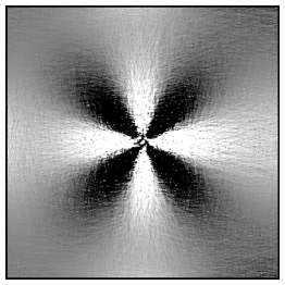
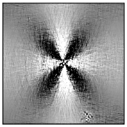
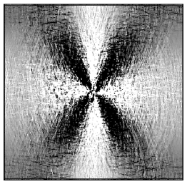
$\varepsilon_{yy}=0.001\%$	$\varepsilon_{yy}=0.505\%$	$\varepsilon_{yy}=0.900\%$
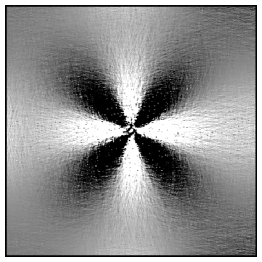
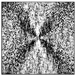
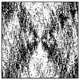
$\varepsilon_{yy}=0.001\%$	$\varepsilon_{yy}=0.239\%$	$\varepsilon_{yy}=0.405\%$
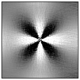
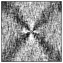
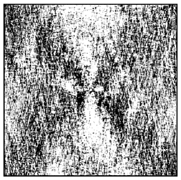
$\varepsilon_{yy}=0.001\%$	$\varepsilon_{yy}=0.142\%$	$\varepsilon_{yy}=0.404\%$

Figure 6: Examples of generated Eshelbies, $N=256\times 256$ grains. Top row: $\mu_{m}=2$, middle row: $\mu_{m}=0.6$, bottom row $\mu_{m}=0.2$. $\bm{\sigma}^{*}$ is coaxial with the load; white grains correspond to a reduction in deviatoric stress. The value of the global strain is given under each panel.

We now focus on the spatial distribution of $\tilde{\sigma}_{yy,i}-\tilde{\sigma}_{xx,i}$ inside the granular sample. In Fig. 6, we show the change in deviatoric stress $\tilde{\sigma}_{yy,i}-\tilde{\sigma}_{xx,i}$. The map is obtained by shading each grain accordingly to the value of the deviatoric stress. The perturbing stress applied in Fig. 6 is $\bm{\sigma}^{*}=\alpha^{*}p_{0}\begin{pmatrix}1&0\\ 0&-1\end{pmatrix}$. Here, $\alpha^{*}$ is a dimensionless number that measures the strength of the perturbation with respect to the confining pressure $p_{0}$. Throughout this paper, $\alpha^{*}=10^{-2}$. Some tests (not shown) were done with $\alpha^{*}=10^{-3}$, and the resulting response is simply divided by 10, indicating that we obtain a linear response.

We considered the biaxial tests of Figs. 2 et 3. For each test, the stress response at three instants are shown: one at the beginning of the test, one near the maximum density (minimum of the curves shown in Fig. 3), and one near the maximum load.

At the beginning of the test, all three tests show a clear, four-lobed pattern characteristic of the Eshelby stress tensor. The dark, maximum stress lobes are oriented at $45^{\circ}$ from the horizontal. After this initial loading, in the case of $\mu_{m}=2$ simulation, the Eshelby pattern remains when the axial strain increases, but the angle of the bands increases. Meanwhile, the other two tests ($\mu_{m}=0.2$ and $0.6$) show a quite different behavior: the band angle remains near $45^{\circ}$, but the texture of the image becomes much more grainy. We will discuss and interpret those different behaviors in section V.

IV.3 Characterization of the angular response

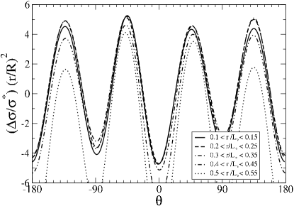
Figure 7: An estimate of the angular dependence of the perturbation stress $f(\theta)$. The stress on grains is averaged over radial bins and then rescaled to esimate $f(\theta)$. This example is for $\mu_{m}=0.6$, $\varepsilon_{yy}=10^{-5}$.

We obtain quantitative information from Fig. 6 about the function $f(\theta)$. We divide the grains into classes according to their distance $r$ from the center of $\mathbb{V}$, and then into subclasses according to their angle $\theta$. An average value of $\Delta\sigma_{i}$ is calculated for each subclass. Then this average is multiplied by the $r^{2}$. This allow us to test the $1/r^{2}$ scaling of the redistributed stress. The resulting function for different classes of $r$ is shown in Fig. 7. We observe a good collapse close to the perturbation ($r\leq 0.35L_{0}$) showing that the far field approximation (leading to keep only the order $1/r^{2}$ for the stress field) is sufficient to capture the radial response. Only the curves corresponding to the largest $r$ differs significantly from the others, certainly because sampled region approaches the boundary of the simulation. (The simulation is approximately square with side length a bit larger than $1.1L_{0}$.)

The scaling in Fig. 7 is based on Eq. (4). This equation shows that the stress response should be proportional to $S/r^{2}$, where $S$ is the area of the inclusion ($S=\pi R^{2}$ in our case). Dividing by $R^{2}/r^{2}$ removes this dependence. Futhermore, the response is proportional to the perturbing stress, so we divide by $\sigma^{*}$ yielding a function $f(\theta)$ of order unity.

We want to identify the position of the maxima of $f(\theta)$. To this end, we consider the grains with $0.1<r/L_{0}<0.3$, and sort them into classes according to their angle $\theta$, and calculate the average change in stress in each class to obtain an estimate of $f(\theta)$. This function is then approximated by a Fourier series

$$f(\theta)\approx a_{0}+\sum_{k=1}^{n}a_{k}\sin k\theta+\sum_{k=1}^{n}b_{k}\cos k\theta,$$ (17)

with $n=8$. The maxima of this Fourier series are identified as the angle of the diagonal bands of the Eshelby.

We study the band angle as a function of loading. As the loading increases, a new problem appears: the packing becomes fragile, and the inclusion can trigger other events throughout the packing that swamp the change in stress caused directly by the inclusion. To get around this problem, we search for times where the packing is relatively stable (absence of kinetic energy peaks), and furthermore, we reduce the strain rate by a factor of 100, so that we will have time to “turn on” the forces in the inclusion.

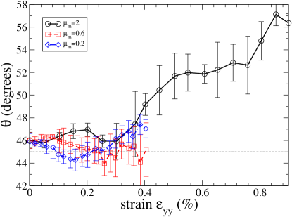
Figure 8: Angle of diagonal bands for simulations with different friction coefficients. For each value of the strain, four angles are averaged together to obtain a mean. The error bars give an idea of the scatter of the different angles measured. The horizontal line indicates an angle of $45^{\circ}$.

In Fig. 8, we show the angle found in this way for the three biaxial tests of Figs. 2 and 3. For each strain value, there are four angles, one for each of the diagonal bands giving its angle relative to the horizontal. These angles are averaged together to obtain a point on the graph. The error bars estimate the scatter of the points; they show the uncertainty of the mean. We observe that at the beginning of the loading all the angles are close to $45^{\circ}$ but with some fluctuations around this value. When the loading increase, the departure from $45^{\circ}$ becomes important. We will further discuss this figure in the next section.

To conclude, the mental construction of Eshelby underlying his computation can be implemented in a numerical simulation of dry frictional disks. In spite of the discrete nature of the material, the continuum mechanics solutions are clearly relevant as the observed response is very similar to the one predicted analytically. This picture is modified when the granular material if further loaded and the friction coefficient decreased.

V Discussion

In this part we discuss the departure from the quadrupolar response observed in Figure 6 either due to the value of the friction coefficient or to the loading of the material. As shown in the previous part, for an isotropically slightly pre-compressed granular material (initial preparation), the response of the material to a localized shear event is compatible with an elastic response (first column of Fig. 6). This picture is modified in two different ways when the material is submitted to an increasing deviatoric stress depending on the value of the friction coefficient. We discuss the different kind of departures from this ideal response in the following.

V.1 Beginning of the loading

As can be seen on the first column of figure 6, at the very beginning of the loading the response is very close to the theoretical prediction recalled in section III.2 and in Figure 4. Quantitatively, as discussed in the preceding section, the radial response is in $1/r^{2}$ and the angular response is dominated by a quadrupolar dependence (Figure 7), with a maximum stress redistribution close to $45^{\circ}$. The direct observation of the stress fields shown in figure 6 shows nevertheless some differences with the response of a continuous material: we can observe that a filamentary pattern underly the smooth response. Consequently, the observed stress redistribution is also compatible with a description of the granular material in term of force chains. The observed striations could indeed indicate that stress is concentrated on grains in force chains. Nevertheless, on a large scale, a smooth quadrupolar response is observed.

As the loading increases, two different behaviors are observed. For $\mu_{m}=2$ (top row), the texture of the patterns remains the same, but the angles depart significantly from $45^{\circ}$. For $\mu_{m}=0.6$ and $\mu_{m}=0.2$, the angles remain close to $45^{\circ}$, but the texture changes significantly. We now discuss these changes.

V.2 Further loading: High value of $\mu_{m}$

When the friction coefficient is artificially high to prevent sliding contacts (upper line of Figure 6), we observe a clear modification of the angles characterizing the stress resdistribution. Meanwhile, the increase in the fluctuations is much smaller than for the smaller friction coefficients. A change of inclination can still be interpreted in an Eshelby picture and we will discuss two possible origins in the following: the effect of the volumetric strain and the effect of anisotropical elasticity.

V.2.1 Polar response and volumetric strain

As discussed in section III.2, the quadrupolar response due to the shear part of the rearrangement is modified by the volumetric contribution. To make explicit this dependence, we study the polar function $f(\theta)$ of Eq. 5. The minima of the function are obtained for $\theta=0^{\circ}[90^{\circ}]$ and the maxima for

$$\cos 2\theta_{E}=\frac{1}{4}\frac{e_{xx}^{*}+e_{yy}^{*}}{e_{yy}^{*}-e_{xx}^{*}}$$ (18)

For the isovolumic case ($e_{xx}^{*}+e_{yy}^{*}=0$), we obtain $\theta_{E}=45^{\circ}[90^{\circ}]$.

Our active inclusions correspond to an imposed traceless stress tensor $\text{Trace}(\bm{\sigma}^{*})=0$. If the inclusion is made of an isotropic elastic material, the associated strain tensor will also be traceless. But the loading process introduces anisotropy into the contact network and thus into the elastic constants, as will be discussed in the next section. In such cases, $\text{Trace}(\bm{e}^{*})$ may be non-zero.

If we suppose that the inclusion changes its volume, a reasonable hypothesis is that $e_{xx}^{*}>0$ and $e_{yy}^{*}<0$, i.e. that the local deformation follows the overall macroscopic deformation. We then obtain for the range of possible values $\theta_{E}\in[\frac{1}{2}\text{acos}\left(\frac{1}{4}\right);\frac{1}{2}\text{acos}\left(-\frac{1}{4}\right)]$, i.e. $\theta_{E}\in[37.8^{\circ};52.2^{\circ}]$. The values greater than $45^{\circ}$ correspond to $e_{xx}^{*}+e_{yy}^{*}>0$, i.e. to dilating plastic events, while the values lesser than $45^{\circ}$ correspond to contracting plastic events. Those two cases are shown on Fig. 4: the angle of the positive part of the deviatoric stress redistribution is indeed smaller than $45^{\circ}$ in the case of a contracting event (Fig. 4(a)) and larger in the case of a dilating one (Fig. 4(b)). The range of possible angles found here correspond to the direction of the maximum of the redistributed deviatoric stress from a single Eshelby inclusion. It differs from the range obtained in Ashwin2013 , where the range of directions of coupled Eshelby inclusion is determined by minimizing the elastic energy of interaction between the inclusions.

The result of this calculation is that only small departure from $45^{\circ}$ can be explained by non-isovolumic transformation. It could for example explain the fluctuations measured in Figure 8 for $\mu_{m}=0.2$ and $\mu_{m}=0.6$ but not the large increase observed in the $\mu_{m}=2$ case.

V.2.2 Anisotropy of the elastic matrix

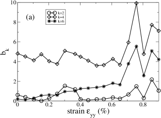
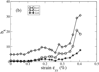
Figure 9: Harmonic components obtained from the fits obtained using equation 17. (a) $\mu_{m}=2$, (b) $\mu_{m}=0.6$ and (c) $\mu_{m}=0.2$.

In this part, we will neglect possible change of volume of the inclusion ($\text{Trace}(\bm{e}^{*})=0$) but we will consider the Eshelby problem in the case of anisotropic elasticity. Indeed, the loading process may induce some anisotropy of the elasticity of the material Acoustics ; LudingMM . The computation of the Green’s function in an anisotropic material is done in Appendix B. Equation 23 shows that in the case of an orthorhombic bidimensional material with a small anisotropy, terms in $2\theta$ and $6\theta$ appear. On the contrary, change of volume of the inclusion do not generate $6\theta$ terms. So the presence of $6\theta$ terms in $f(\theta)$ may be viewed as an indication of anisotropic elasticity. This can be checked by the Fourier analysis done in section IV.3 (fit of the measured response by equation 17). The different components of the fit are shown in Figure 9. We observe that indeed the $6\theta$ component is the second most important harmonic in the case of $\mu_{m}=2$. This supports the hypothesis that the observed modification of the angle is due to the effect of material anisotropy, and not to volume change of the inclusion.

This effect is less clear for $\mu_{m}=0.6$ and $\mu_{m}=0.2$ where the second dominant harmonic is $2\theta$ which can originate both from volumetric effects and anisotropical effects. In fact, for those values of $\mu_{m}$, the principal effect of the loading is not modification of the angles (that fluctuate close to $45^{\circ}$ - see Figure 8) but rather the increase of fluctuations (see Figure 6) as will be discussed in the next part.

V.3 Further loading: Low value of $\mu_{m}$

For $\mu_{m}=0.6$ and $\mu_{m}=0.2$ at intermediate and large values of the strain (lower right four panels in Fig. 6) the filamentary striations visible in the other panels of Fig. 6) are replaced by a grainy strongly fluctuating texture. In spite of this, the response at large scales remains quadrupolar, with angles close to $45^{\circ}$.

This change in texture cannot be described in the Eshelby formalism, which supposes that the material is continuous. We do not think that this difference of texture is due to the disorder of the contacts between grains, but likely due to sliding contacts. Indeed, the $\mu_{m}=0.2$ and $\mu_{m}=0.6$, there are many sliding contacts (up to $35\%$ and $15\%$ of all contacts, respectively) but at $\mu_{m}=2$, sliding contacts remain relatively rare (less than $2.5\%$ of all contacts).

The permanence of the quadrupolar structure at large scale shows than an elastic description of a granular material can co-exist with different mesoscopic behaviors: either force chains ($\varepsilon_{yy}=10^{-5}$ or $\mu_{m}=2$) or sliding contacts (large $\varepsilon_{yy}$ and $\mu_{m}=0.2,0.6$). When many contacts are sliding, the granular matrix does not behave as an elastic material. We then expect a stress redistribution which differs from the elastic Eshelby response. However, at large scales, we still see in Fig. 6 the Eshelby structure which is a characteristic of the material elasticity. It is unclear if it is possible to quantify objectively such a separation of scales.

VI Conclusion

In this paper, we considered the effect of a local transformation on the mechanical stress distribution. For this, we applied the theoretical construction proposed by Eshelby to numerical simulations where extra forces are applied on some grains inside a granular material. In response to this local applied stress, the material relaxes stress at large distance. This stress relaxation may be, at least in some cases, successfully described by a theory where the granular material is treated as a continuous and elastic material. The presence of disorder of contact forces (such as the so called force-chains) does not disrupt this elastic response, at least at the macroscopic scale. If sliding contacts are supressed, we show that the material remains elastic at the macroscopic scale, even close to failure, but the elastic coefficients become anisotropic.

Our numerical simulations are performed with beads of finite stiffness. The ratio $p_{0}/k_{N}=5.10^{-4}$ between the confining pressure and the contact stiffness, is the typical value of the relative deformations of the beads. It is interesting to compare it to a real 3D experiment. If we consider glass beads following Hertz law which are confined under a pressure $P=100~{}kPa$, we may estimate a relative deformation of the beads of $3.10^{-4}$. So the value of the relative deformation is of the same order of magnitude as many biaxial compression experiments, such as experiments where stress relaxations along preferential directions are observed LeBouil2014 ; LeBouil2014b .

Some departures from the elastic behavior are clearly visible in our simulations. They may be linked to the occurrence of sliding contacts. The departure from an elastic response of the matrix is an interesting, but very challenging, problem. We may expect that the granular skeleton behaves elastically for deformations of the inclusion which are smaller than some plasticity threshold $\varepsilon_{th}$. The variation of $\varepsilon_{th}$ with the microscopic friction coefficient $\mu_{m}$, with the reduced stiffness of the beads $p_{0}/k_{N}$, and with the proximity of the material failure are still unknown. This will be the subject of a future work.

Appendix A Computation of the released stress

The bidimensional Green function is:

$$G_{ij}^{(2D)}(\vec{r}-\vec{r^{\prime}})=\frac{1}{4\pi\mu}\frac{\lambda+\mu}{\lambda+2\mu}\left[-\frac{\lambda+3\mu}{\lambda+\mu}\delta_{ij}\ln|\vec{r}-\vec{r^{\prime}}|+\frac{(x_{i}-x_{i}^{\prime})(x_{j}-x_{j}^{\prime})}{|\vec{r}-\vec{r^{\prime}}|^{2}}\right]$$ (19)

where $\vec{r}=\left(\begin{array}[]{c}x\\ y\end{array}\right)=\left(\begin{array}[]{c}r\cos\theta\\ r\sin\theta\end{array}\right)$ are the coordinates in the bidimensional plane.

The displacement field in the matrix can be obtained by integrating the Green function along the contour $C$ of the inclusion:

$$\tilde{u}_{i}(\vec{r}) = \frac{1}{4\pi\mu}\frac{\lambda+\mu}{\lambda+2\mu}\oint_{C}\left[-\frac{\lambda+3\mu}{\lambda+\mu}\delta_{ij}\ln|\vec{r}-\vec{r^{\prime}}|+\frac{(x_{i}-x_{i}^{\prime})(x_{j}-x_{j}^{\prime})}{|\vec{r}-\vec{r^{\prime}}|^{2}}\right]\sigma_{jk}^{*}dc_{k}^{\prime}$$

$$= \frac{\sigma_{jk}^{*}}{4\pi\mu}\frac{\lambda+\mu}{\lambda+2\mu}\iint_{S}\left[\frac{\lambda+3\mu}{\lambda+\mu}n_{k}\delta_{ij}+\left(-\delta_{ik}n_{j}-\delta_{jk}n_{i}+2n_{i}n_{j}n_{k}\right)\right]\frac{dS^{\prime}}{|\vec{r}-\vec{r^{\prime}}|}$$

Where $\vec{n}=\frac{\vec{r}-\vec{r^{\prime}}}{|\vec{r}-\vec{r^{\prime}}|}$. Using $\sigma_{ij}^{*}=\lambda e_{ll}^{*}\delta_{ij}+2\mu e_{ij}^{*}$ one obtains:

$$\tilde{u}_{i}(\vec{r})=\frac{e_{jk}^{*}}{2\pi}\frac{\lambda+\mu}{\lambda+2\mu}\iint_{S}\left[\frac{\mu}{\lambda+\mu}(\delta_{ij}n_{k}+\delta_{ik}n_{j}-\delta_{jk}n_{i})+2n_{i}n_{j}n_{k}\right]\frac{dS^{\prime}}{|\vec{r}-\vec{r^{\prime}}|}$$ (20)

Consequently, far from the inclusion, we can write:

$$\tilde{u_{i}}(\vec{r})=\frac{S}{2\pi r}\frac{\lambda+\mu}{\lambda+2\mu}e_{jk}^{*}g_{ijk}^{2D}(\vec{n})$$ (21)

with $g_{ijk}^{2D}(\vec{n})=\frac{\mu}{\lambda+\mu}(\delta_{ij}n_{k}+\delta_{ik}n_{j}-\delta_{jk}n_{i})+2n_{i}n_{j}n_{k}$.

For the particular case when $\mathbf{e^{*}}=\left(\begin{array}[]{cc}e^{*}_{xx}&0\\ 0&e^{*}_{yy}\\ \end{array}\right)$ we have:

$$\tilde{u}_{r}(\vec{r}) = \frac{S}{2\pi r}\frac{\lambda+\mu}{\lambda+2\mu}\left[\frac{\lambda+2\mu}{\lambda+\mu}(e_{xx}^{*}-e_{yy}^{*})\cos 2\theta+(e_{xx}^{*}+e_{yy}^{*})\right]$$

$$\tilde{u}_{\theta}(\vec{r}) = \frac{S}{2\pi r}\frac{\lambda+\mu}{\lambda+2\mu}\left[-\frac{\mu}{\lambda+\mu}(e_{xx}^{*}-e_{yy}^{*})\sin 2\theta\right]$$

The components of the strain tensor in polar coordinates are then:

$$\tilde{e}_{rr} = \frac{S}{2\pi r^{2}}\frac{\lambda+\mu}{\lambda+2\mu}\left[-\frac{\lambda+2\mu}{\lambda+\mu}(e_{xx}^{*}-e_{yy}^{*})\cos 2\theta-(e_{xx}^{*}+e_{yy}^{*})\right]$$

$$\tilde{e}_{\theta\theta} = \frac{S}{2\pi r^{2}}\frac{\lambda+\mu}{\lambda+2\mu}\left[\frac{\lambda}{\lambda+\mu}(e_{xx}^{*}-e_{yy}^{*})\cos 2\theta+(e_{xx}^{*}+e_{yy}^{*})\right]$$

$$\tilde{e}_{r\theta} = \frac{S}{2\pi r^{2}}\frac{\lambda+\mu}{\lambda+2\mu}\left[-(e_{xx}^{*}-e_{yy}^{*})\sin 2\theta\right]$$

using $\tilde{e}_{xx}-\tilde{e}_{yy}=\cos(2\theta)\left(\tilde{e}_{rr}-\tilde{e}_{\theta\theta}\right)-2\sin(2\theta)\tilde{e}_{r\theta}$, we obtain for the deviatoric strain:

$$\tilde{e}_{xx}-\tilde{e}_{yy}=\frac{S}{\pi r^{2}}\frac{\lambda+\mu}{\lambda+2\mu}\left[-(e_{xx}^{*}-e_{yy}^{*})\cos 4\theta-(e_{xx}^{*}+e_{yy}^{*})\cos 2\theta\right]$$ (22)

Appendix B Eshelby inclusion in an anisotropic material

We consider the case of an orthorhombic bidimensional material which free energy is of the form Landau :

$$F=\frac{1}{2}\lambda_{xxxx}e_{xx}^{2}+\frac{1}{2}\lambda_{yyyy}e_{yy}^{2}+\lambda_{xxyy}e_{xx}e_{yy}+2\lambda_{xyxy}e_{xy}^{2}$$

From the equilibrium equations $\frac{\partial\sigma_{ik}}{\partial x_{k}}+b_{i}=0$, where $b_{i}$ is a body force, we can then deduce

$$\lambda_{xxxx}\frac{\partial^{2}u_{x}}{\partial x^{2}}+\lambda_{xyxy}\frac{\partial^{2}u_{x}}{\partial y^{2}}+(\lambda_{xxyy}+\lambda_{xyxy})\frac{\partial^{2}u_{y}}{\partial x\partial y}+b_{x} = 0$$

$$\lambda_{yyyy}\frac{\partial^{2}u_{y}}{\partial y^{2}}+\lambda_{xyxy}\frac{\partial^{2}u_{y}}{\partial x^{2}}+(\lambda_{xxyy}+\lambda_{xyxy})\frac{\partial^{2}u_{x}}{\partial x\partial y}+b_{y} = 0$$

To find the Green’s function of this system, i.e. the solution of the system when $b_{i}=n_{i}\delta(\vec{r})$ where $\vec{n}$ is a vector of unit norm, we work in the Fourier space. Noting the Fourier transform of the components of the Green tensor $\mathbb{G}_{ij}$, we obtain the following relations:

$$\lambda_{xxxx}q_{x}^{2}\mathbb{G}_{xx}+\lambda_{xyxy}q_{y}^{2}\mathbb{G}_{xx}+(\lambda_{xxyy}+\lambda_{xyxy})q_{x}q_{y}\mathbb{G}_{yx} = \frac{1}{4\pi^{2}}$$

$$\lambda_{xxxx}q_{x}^{2}\mathbb{G}_{xy}+\lambda_{xyxy}q_{y}^{2}\mathbb{G}_{xy}+(\lambda_{xxyy}+\lambda_{xyxy})q_{x}q_{y}\mathbb{G}_{yy} = 0$$

$$\lambda_{yyyy}q_{y}^{2}\mathbb{G}_{yy}+\lambda_{xyxy}q_{x}^{2}\mathbb{G}_{yy}+(\lambda_{xxyy}+\lambda_{xyxy})q_{x}q_{y}\mathbb{G}_{xy} = \frac{1}{4\pi^{2}}$$

$$\lambda_{yyyy}q_{y}^{2}\mathbb{G}_{yx}+\lambda_{xyxy}q_{x}^{2}\mathbb{G}_{yx}+(\lambda_{xxyy}+\lambda_{xyxy})q_{x}q_{y}\mathbb{G}_{xx} = 0$$

The components $\mathbb{G}_{yx}$ can be deduced from those relations. We compute them in the case of small anisotropy, i.e. when $\lambda_{xxxx}-\lambda_{xxyy}-2\lambda_{xyxy}$ and $\lambda_{yyyy}-\lambda_{xxyy}-2\lambda_{xyxy}$ are small Landau . We then write:

$$\lambda_{xxxx}=\lambda+2\mu-\epsilon\hskip 28.45274pt\lambda_{yyyy}=\lambda+2\mu+\epsilon\hskip 28.45274pt\lambda_{xxyy}=\lambda\hskip 28.45274pt\lambda_{xyxy}=\mu$$

with $\epsilon\ll\lambda,\mu$. We obtain then

$$\mathbb{G}_{xx} = \frac{1}{4\pi^{2}\mu}\left(\frac{1}{q^{2}}-\frac{\lambda+\mu}{\lambda+2\mu}\frac{q_{x}^{2}}{q^{4}}\right)\left[1+\frac{\epsilon}{\lambda+2\mu}\frac{q_{x}^{2}}{q^{2}}\left(1+\frac{(\lambda+\mu)q_{y}^{2}}{(\lambda+\mu)q_{y}^{2}+\mu q^{2}}\right)\right]$$

$$\mathbb{G}_{yy} = \frac{1}{4\pi^{2}\mu}\left(\frac{1}{q^{2}}-\frac{\lambda+\mu}{\lambda+2\mu}\frac{q_{y}^{2}}{q^{4}}\right)\left[1-\frac{\epsilon}{\lambda+2\mu}\frac{q_{y}^{2}}{q^{2}}\left(1+\frac{(\lambda+\mu)q_{x}^{2}}{(\lambda+\mu)q_{x}^{2}+\mu q^{2}}\right)\right]$$

$$\mathbb{G}_{xy}=\mathbb{G}_{yx} = -\frac{1}{4\pi^{2}\mu}\frac{\lambda+\mu}{\lambda+2\mu}\frac{q_{x}q_{y}}{q^{4}}\left[1+\frac{\epsilon}{\lambda+2\mu}\frac{q_{x}^{2}-q_{y}^{2}}{q^{2}}\right]$$

We have $\hat{e}_{il}^{*}=4\pi^{2}Sq_{k}q_{l}\mathbb{G}_{ij}\sigma_{jk}^{*}$ Picard2004 with $S$ the surface of the inclusion, from which we deduce:

$$\hat{e}_{xx}-\hat{e}_{yy}=-\frac{S\sigma^{*}}{\mu}\left[1-\frac{\lambda+\mu}{\lambda+2\mu}\frac{(q_{x}^{2}-q_{y}^{2})^{2}}{q^{4}}+\frac{\epsilon}{\lambda+2\mu}\left(\frac{q_{x}^{2}-q_{y}^{2}}{q^{2}}-\frac{\lambda+\mu}{\lambda+2\mu}\frac{(q_{x}^{2}-q_{y}^{2})^{3}}{q^{6}}\right)\right]$$ (23)

for $\bm{\sigma^{*}}=\left(\begin{array}[]{cc}\sigma^{*}&0\\ 0&-\sigma^{*}\\ \end{array}\right)$.

The first isotropical term on the right hand side of eq. 23 Fourier transform leads to a Dirac term in $\vec{r}=\vec{0}$. It is in fact due to the ponctual plastic event in the inclusion and should be removed when computing the elastic response Picard2004 . The $\frac{(q_{x}^{2}-q_{y}^{2})^{2}}{q^{4}}$ leads to a $\frac{\cos 4\theta}{r^{2}}$ term in the real space Picard2004 . It differs from the usual form $\frac{q_{x}^{2}q_{y}^{2}}{q^{4}}$ obtained in simple shear configuration because the pattern is rotate of $45^{\circ}$ in a biaxial loading compare to simple shear. We thus recover the quadrupolar response for an isovolumic inclusion in absence of anisotropy ($\epsilon=0$).

The term of order $\epsilon$ gives the modification of the response due to the anisotropy of the matrix. From symetry arguments, we see that those terms will give rise in the real space to terms of the form $\frac{\cos 2\theta}{r^{2}}$ and $\frac{\cos 6\theta}{r^{2}}$.

References

- (1) Critical State Soil Mechanics, A. N. Schofield, & C. P. Wroth (McGraw-Hill, 1968).
- (2) Statics and Kinematics of Granular Materials, R. M. Nedderman (Cambridge University Press, 1992).
- (3) Plasticity and geomechanics, R. O. Davis and A. P. S. Selvadurai (Cambridge University Press, 2002).
- (4) Bifurcation analysis in geomechanics, I. Vardoulakis and J. Sulem (Blackie Academic and Professional, Glasgow, England , 1995).
- (5) K. Kamrin, and G. Koval, Phys. Rev. Lett. 108, 178301 (2012).
- (6) M. Bouzid, A. Izzet, M. Trulsson, E. Clément, P. Claudin, B. Andreotti, Eur. Phys. J. E 38, 125 (2015).
- (7) A. S. Argon, Acta Metall. 27, 47 (1979).
- (8) A. S. Argon and H. Y. Kuo, Mater. Sci. Engng. 39, 101 (1979).
- (9) M. L. Falk, and J. S. Langer, Phys. Rev. E 57, 7192–7205 (1998).
- (10) C. E. Maloney, & A. Lemaître, Phys. Rev. E 74, 016118 (2006).
- (11) A. Tanguy, F. Leonforte, and J.-L. Barrat, Eur. Phys. J. E 20, 355 (2006).
- (12) P. Schall, D. A. Weitz, and F. Spaepen, Science 318, 1895 (2007).
- (13) A. Amon, V. B. Nguyen, A. Bruand, J. Crassous, and E. Clément, Phys. Rev. Lett. 108, 135502 (2012).
- (14) K. E. Jensen, D. A. Weitz, and F. Spaepen, Phys. Rev. E 90, 042305 (2014).
- (15) Kenneth W. Desmond and Eric R. Weeks, Phys. Rev. Lett. 115,098302 (2015).
- (16) G. Picard, A. Ajdari, F. Lequeux, and L. Bocquet, Eur. Phys. J. E 15, 371 (2004).
- (17) A. Nicolas, J. Rottler, and J.-L. Barrat, European Physical Journal E 37,6 (2014).
- (18) F. Puosi, J. Olivier, and K. Martens, Soft Matter 11,7639 (2015).
- (19) J. Lin, E. Lerner, A. Rosso, M. Wyart, Proc. Nat. Acad. Sci. Am. 111,14382 (2014).
- (20) J. Lin, T. Gueudré, A. Rosso, and M. Wyart, Phys. Rev. Lett. 115,168001 (2015).
- (21) T. Sentjabrskaja, P. Chaudhuri, M. Hermes, W. C. K. Poon, J. Horbach, S. U. Egelhaaf and M. Laurati , Scientific Reports 5,11884 (2015).
- (22) A. Kabla and G. Debrégeas, Phys. Rev. Lett. 90, 258303 (2003).
- (23) A. Le Bouil et al., Granular Matter 16, 1-8 (2014).
- (24) A. Le Bouil et al., Phys. Rev. Lett. 112, 246001 (2014).
- (25) J. D. Eshelby, Proc. R. Soc. Lond. A 241, 376-396 (1957).
- (26) R. Dasgupta, H. Hentschel, E. George and I. Procaccia, Phys. Rev. E 87, 022810 (2013).
- (27) R. Dasgupta, O. Gendelman, P. Mishra, I. Procaccia, and C. Shor, Phys. Rev. E 88, 032401 (2013).
- (28) S. Alexander Physics Reports 296 65-236, Sec. 4.3 (1998)
- (29) J. Ashwin, O. Gendelman, I. Procaccia, and C. Shor, Phys. Rev. E 88, 022310 (2013).
- (30) F. Puosi, J. Rottler, and J.-L. Barrat, Phys. Rev. E 89, 042302 (2014).
- (31) N. V. Priezjev, Phys. Rev. E 91, 032412 (2015).
- (32) B. Wu, T. Iwashita, and T. Egami , Phys. Rev. E 91,032301 (2015).
- (33) N. Guo and J. Zhao, Phys. Rev. E 89,042208 (2014)
- (34) M. R. Kuhn, Mechanics of Materials 31, 407 (1999)
- (35) T. W. Lambe and R. V. Whitman, Soil Mechanics (John Wiley & Sons, New York, 1979).
- (36) J. Desrues and E. Andò, C. R. Phys. 16, 26 (2015).
- (37) T. S. Majmudar et al., Phys. Rev. Lett. 98, 058001 (2007).
- (38) S. McNamara in III International Conference on Particle-based Methods: Fundamentals and Applications PARTICLES 2013 M. Bischoff, E. Oñate, D.R.J. Owen, E. Ramm & P. Wriggers (Eds).
- (39) Théorie de l’élasticité L. Landau & E. Lifchitz (Mir, 1967, Moscou).
- (40) S. McNamara, Granular Matter 17 311 (2015).
- (41) S. Luding, Int. J. Sol. Struct. 41 5821-5836 (2004).