X-ray observations of dust obscured galaxies in the Chandra Deep Field South

We present the properties of X-ray detected dust obscured galaxies (DOGs) in the Chandra Deep Field South. In recent years, it has been proposed that a significant percentage of the elusive Compton-thick (CT) active galactic nuclei (AGN) could be hidden among DOGs. This type of galaxy is characterized by a very high infrared (IR) to optical flux ratio ($f_{24\mu m}/f_{R}>1000$), which in the case of CT AGN could be due to the suppression of AGN emission by absorption and its subsequent re-emission in the IR. The most reliable way of confirming the CT nature of an AGN is by X-ray spectroscopy. In a previous work, we presented the properties of X-ray detected DOGs by making use of the deepest X-ray observations available at that time, the 2Ms observations of the Chandra deep fields, the Chandra Deep Field North (CDF-N), and the Chandra Deep Field South (CDF-S). In that work, we only found a moderate percentage ($<$ 50%) of CT AGN among the DOGs sample. However, we pointed out that the limited photon statistics for most of the sources in the sample did not allow us to strongly constrain this number. In this paper, we further explore the properties of the sample of DOGs in the CDF-S presented in that work by using not only a deeper 6Ms Chandra survey of the CDF-S, but also by combining these data with the 3Ms XMM-Newton survey of the CDF-S. We also take advantage of the great coverage of the CDF-S region from the UV to the far-IR to fit the spectral energy distributions (SEDs) of our sources. Out of the 14 AGN composing our sample, 9 are highly absorbed ( N_H $>$ 10²³ cm^-2), whereas 2 look unabsorbed, and the other 3 are only moderately absorbed. Among the highly absorbed AGN, we find that only three could be considered CT AGN. In only one of these three cases, we detect a strong Fe K$\alpha$ emission line; the source is already classified as a CT AGN with Chandra data in a previous work. Here we confirm its CT nature by combining Chandra and XMM-Newton data. For the other two CT candidates, the non-detection of the line could be because of the low number of counts in their X-ray spectra, but their location in the L${}_{\rm 2-10\,keV}$/L_12μm plot supports their CT classification. Although a higher number of CT sources could be hidden among the X-ray undetected DOGs, our results indicate that DOGs could be as well composed of only a fraction of CT AGN plus a number of moderate to highly absorbed AGN, as previously suggested. From our study of the X-ray undetected DOGs in the CDF-S, we estimate a percentage between 13 and 44% of CT AGN among the whole population of DOGs.

1 Introduction

There is mounting evidence that the growth of galaxies and the super-massive black holes (SMBHs) at their centres must be strongly connected (Magorrian et al. 1998, Ferrarese & Merritt 2000, Gebhardt et al. 2000, Tremaine et al. 2002, Tremaine et al. 2002, Marconi et al. 2004, Ferrarese & Ford 2005, Kormendy & Ho 2013). Moreover, star formation history seems to follow that of SMBH growth via accretion and traced by active galactic nuclei (AGN) emission (La Franca et al. 2005). Therefore, to obtain a complete census of the AGN population is vital to understand cosmic evolution.

X-rays surveys are extremely efficient in finding AGN since X-rays are able to penetrate high amounts of gas and dust. Nevertheless, X-ray surveys, even the deepest, such as the Chandra Deep Field Surveys, and the hardest (i.e., those carried out above 10 keV), are still biased against the most heavily absorbed AGN, the so-called Compton-thick (CT) AGN (column densities N_H $>$ 10²⁴ cm^-2). The actual percentage of CT AGN among the AGN population is still unknown and it is usually inferred in an indirect way from the modelling of the cosmic X-ray background (CXB; see Gilli et al. 2007, Treister et al. 2009b, Akylas et al. 2012).

In the past few years, mid-infrared (IR) surveys have been proposed as an alternative way of finding and studying CT AGN. The AGN emission that is absorbed is then re-emitted by the heated dust, so CT AGN, given their extremely obscured nature, should emit strongly in the mid-IR while they are fainter at other wavelengths. This has been the basic selection argument used in several recent works. For example, Martínez-Sansigre et al. (2005) argued that the missing AGN obscured population at high redshifts displays bright 24 $\mu m$ emission with no 3.6 $\mu m$ detection. Daddi et al. (2007a) used ultraviolet (UV) selected sources instead and found a very high percentage of CT AGN among those showing mid-IR excess.

In this work, we focus on mid-IR bright optically faint sources that have been associated with dust obscured galaxies (DOGs). DOGs were first discovered using Spitzer data (Houck et al. 2005), as a population of 24 $\mu m$ bright, R-band faint sources at redshifts $z\approx 2$ (with a small scatter $\sigma_{z}=0.5$; Dey et al. 2008, Pope et al. 2008); this implies luminosities $\rm L_{IR}>10^{12-14}L_{\odot}$ that are comparable or in excess of low redshift ultra-luminous infrared galaxies (ULIRGs; Sanders & Mirabel 1996). At those redshifts, the 24 $\mu m$ emission corresponds to the peak of the torus IR emission in AGN. Therefore, this selection technique should be very efficient in detecting heavily obscured AGN.

Fiore et al. (2008) proposed that most of the DOGs may be CT AGN. The stacked X-ray signal of the undetected DOGs in X-ray surveys appears to be flat, which is indicative of absorbed sources (Fiore et al. 2008, Georgantopoulos et al. 2008, Fiore et al. 2009, Treister et al. 2009a). However, Georgantopoulos et al. (2008) pointed out that a flat stacked spectrum could also be produced by a combination of low-luminosity AGN with moderate absorption. Moreover, Pope et al. (2008) showed that the normal galaxy (non-AGN) content of DOG samples may still be significant. In any case, the most reliable way to confirm their CT AGN nature is to obtain their intrinsic absorption, or a strong Fe K$\alpha$ emission line detection, directly from X-ray spectroscopy (see for example Fukazawa et al. 2011).

Lanzuisi et al. (2009) performed an X-ray study of 44 luminous DOGs ($F_{24\mu m}/F_{R}>2000$ and $F_{24\mu m}>1.3$ mJy ) in the Spitzer Wide-Area Infrared Extragalactic (SWIRE) survey, of which 23 are detected in X-rays. Among the DOGs detected in X-rays, half of these have column densities $\rm N_{H}>10^{23}$ $\rm cm^{-2}\leavevmode\nobreak\$, but only one could be classified as a CT AGN. Fiore et al. (2009) investigated the X-ray properties of 73 DOGs in the Cosmic Evolution Survey (COSMOS) (Elvis et al. 2009). They derived their column densities from hardness ratios, directly for the 31 detected in X-rays and from stacked images from the undetected DOGs, and found that the fraction of CT AGN among DOGs seems to increase as their IR luminosity increases. This is consistent with previous and more recent results in which the percentage of AGN has been found to increase as the IR luminosity increases (Sacchi et al. 2009; Lee et al. 2010; Riguccini et al. 2015). Lanzuisi et al. (2009) also found that the hardness ratios of X-ray undetected DOGs were consistent with those of the detected DOGs, and these authors argued that the very flat photon index in both samples indicates a high percentage of CT AGN among DOGs.

Georgakakis et al. (2010) compiled a sample of “low redshift DOGs analogues” from the AEGIS and CDF-N surveys. These are sources for which their spectral energy distributions (SEDs) would be similar to those of DOGs if placed at redshift 2. Nine of their sources have X-ray counterparts, and only three of these sources show tentative evidence of CT obscuration. The SEDs of the X-ray undetected DOGs are consistent with starburst activity showing no evidence for a hot dust component. Georgakakis et al. (2010) concluded that there is little evidence for the presence of a high percentage of luminous CT sources in either the X-ray detected or undetected population of DOGs analogues.

Finally, Treister et al. (2009a) examine the properties of 211 heavily obscured AGN candidates in the extended CDF-S, selecting objects with $f_{24\mu m}/f_{R}>1000$ and $R-K>4.5$. Eighteen sources are detected in X-rays, they have moderate column densities $\sim 10^{22-23}$ $\rm cm^{-2}\leavevmode\nobreak\$, and only two of these sources appear to be CT. The X-ray undetected sources show a hard average spectrum that could be interpreted as a mixture of 90% CT objects and 10% star-forming galaxies.

In our previous work (Georgantopoulos et al. 2011), we presented the properties of 26 X-ray detected DOGs from the 2Ms surveys in the CDF-N and CDF-S and we found only a moderate percentage of CT AGN, although at least half of the full sample show signs of heavy (but Compton-thin) obscuration. It has to be noted that, because of poor photon statistics, in many cases a heavily absorbed nature was inferred from a very flat spectrum. We also found that the average spectrum of X-ray detected and undetected DOGs are very similar with a very hard photon index. This could indicate a high percentage of CT sources, but also a combination of a moderate percentage of CTs plus a higher number of only moderately absorbed AGN.

Here we further explore the properties of the X-ray detected DOGs in the CDF-S presented in Georgantopoulos et al. (2011) by combining 6 Ms Chandra and 3 Ms XMM-Newton observations of this region, and thus, by taking advantage of the improved signal-to-noise ratio of the new X-ray spectra. We adopt H_o =75 km s^-1, $\Omega_{M}$ = 0.3, and $\Omega_{\Lambda}$ = 0.7 throughout this paper. Errors are reported at the 90% confidence level.

2 Chandra Deep Field South

Chandra Deep Field South (CDF-S) is the deepest Chandra survey to date, covering an area of 465 arcmin². The most recent catalogue of X-ray sources within the CDF-S was produced by using 52 observations with a total exposure time of $\sim$ 4 Ms (Xue et al. 2011). A further approved 3 Ms is due to be added to this field, which will bring the total exposure to 7 Ms by the end of 2015. This area has also been observed by XMM-Newton with a total exposure time of $\sim$ 3 Ms (Ranalli et al. 2013). The flux limits in the hard (Chandra: 2-8 KeV, XMM-Newton: 2-10 keV) band for these surveys are 5.5$\times$10^-17 erg cm^-2 s^-1 and 6.6$\times$10^-16 erg cm^-2 s^-1 for the Chandra and XMM-Newton observations, respectively. To maximize the spectral quality of our sample, we extracted spectral data from all the Chandra observations that were publicly available by June 2015, which resulted in a maximum exposure time of $\sim$ 6 Ms.

This area has also extensive multi-wavelength coverage from the UV to the far-IR. Near-UV to near-IR data are available from the GOODS-MUSIC catalogue (Grazian et al. 2006), including U photometry from ESO-La Silla and ESO-VLT-VIMOS; B, V, i, and z photometry from HST-ACS; J, H, and K photometry from VLT-ISAAC; and Spitzer photometry at 3.5, 4.5, 5.8, 8 $\mu m$ (IRAC), and 24 $\mu m$ (MIPS). We also used more recent Spitzer-IRAC observations from the SIMPLE survey (Damen et al. 2011) and optical data from the MUSYC catalogue (Gawiser et al. 2006). Far-IR data in the 100 and 160 $\mu m$ bands are available from the GOODS-Herschel survey (Elbaz et al. 2007), and the PACS Evolutionary Probes programme (Lutz et al. 2011).

3 Sample of dust obsured galaxies

Our sample of X-ray detected DOGs is composed of the 14 sources in the CDF-S studied in Georgantopoulos et al. (2011). For seven of these sources, there are data available from both XMM-Newton and Chandra observations. The selection of the sample is described in detail in Georgantopoulos et al. (2011). We combined the catalogue in Grazian et al. (2006) with the X-ray catalogue of Luo et al. (2008, 2010), which is based on the 2 Ms Chandra catalogue, and selected those sources with log($f_{24\mu m}$/f_R) $>$ 3 with a lower limit for optical non-detections of R = 26.5(AB). There are 56 additional DOGs within the CDF-S footprint with no X-ray counterpart in the 2 Ms Chandra catalogue, four of these now detected using the 4 Ms Chandra data (Xue et al. 2011). However, the X-ray data quality of these new four X-ray detected DOGs is too poor to perform a reliable spectral analysis, which is the purpose of this work, so we refer to these sources as X-ray undetected DOGs in this paper.

Only Chandra spectral data from the 2 Ms survey was used in Georgantopoulos et al. (2011). Here we combine 6 Ms of Chandra data with the 3 Ms of XMM-Newton data to better constrain the absorption properties of the X-ray detected DOGs. The X-ray observations of the DOGs in our sample are listed in Table 1. Redshifts were extracted from Hsu et al. (2014), spectroscopic redshifts being available only for four of the sources.

Table 1: X-ray observations of the DOGs sample

LID	PID	RA	DEC	z	$f_{2-10\,{\rm keV}}$	Cts(Chandra)	Cts (XMM)
(1)	(2)	(3)	(3)	(4)	(5)	(6)	(7)
95	325	53.0349	-27.6796	5.22	4.3	257	385
117	(225)	53.0491	-27.7745	1.51	2.5	964	-
170	-	53.0720	-27.8189	1.22	0.1	20	-
197	140	53.0916	-27.8532	1.81	0.6	125	126
199	(193)	53.0923	-27.8032	2.45	0.6	213	-
230	-	53.1052	-27.8752	2.61	0.1	48	-
232	283	53.1070	-27.7183	2.291	4.6	1791	2279
293	-	53.1394	-27.8744	3.88	0.2	81	-
307	102	53.1467	-27.8883	1.90	1.6	697	332
309	172	53.1488	-27.8211	2.579	1.2	129	131
321	118	53.1573	-27.8700	1.603	13.0	7661	9253
326	-	53.1597	-27.9313	3.10	0.8	254	-
346	64	53.1703	-27.9297	1.221	5.8	1549	1581
397	(74)	53.2049	-27.9180	2.28	2.1	510	-

• The columns are: (1) Chandra ID from the Luo et al. (2010) catalogue. (2) XMM ID from the Ranalli et al. (2013) catalogue; numbers in brackets denote sources that are detected by XMM-Newton but with a limited number of counts (so no spectral fit has been carried out). (3) X-ray coordinates (J2000). (4) Redshift: two decimal and three decimal digits denote photometric and spectroscopic redshifts, respectively. (5) 2-10 keV Chandra flux in units of $10^{-15}$ $\rm erg\,cm^{-2}\,s^{-1}$ from the Luo et al. (2010) catalogue. (6) Background subtracted Chandra counts in the total band 0.3-8 keV (7) Background subtracted XMM-Newton EPIC(MOS+pn) counts in the 0.3-8 keV band.

4 X-ray Spectroscopy

To maximize the spectral quality of our sample, we extracted spectral data from all the Chandra observations publicly available by June 2015. In particular, we reduced all the Chandra survey data in a uniform manner, screening for hot pixels and cosmic afterglows as described in Laird et al. (2009) with the CIAO data analysis software version 4.8. We used the SPECEXTRACT script in the CIAO package to extract spectral information from the individual CDF-S observations. The extraction radius increases with off-axis angle to enclose 90% of the PSF at 1.5 keV. The same script extracts response and auxiliary files. The background spectrum was estimated from source free regions of the image for each observation. The spectra from each observation were then merged to create a single source spectrum, background spectrum, response, and auxiliary matrices for each source using the FTOOL tasks MATHPHA, ADDRMF, and ADDARF, respectively. The addition of the spectra from all observations results in a maximum exposure of $\sim$6 Ms. However, sources near the edges of the field may not be present in all individual observations because the aim points and roll angles vary between observations. In these cases, the total exposure is significantly smaller.

We used Xspec v12.8 (Arnaud 1996) to carry out the spectral analysis. We selected Cash statistics instead of the most commonly used $\chi^{2}$ statistic to obtain reliable spectral results even for very low count data.

The initial model was a power law modified by photoelectric absorption at the source redshift. We modelled this absorption using the Xspec model plcabs, which properly takes not only absorption but also Compton scattering into account, and can be applied up to column densities $\sim$ 5$\times$10²⁴ cm^-2. If column densities were found to be higher than this value, we attempted to use the torus absorption model described in Brightman & Nandra (2011), which can be applied for higher column densities. We also added a second power law, when neccessary, to account for soft scattered emission. We fixed the photon index to 1.8 in all cases (Tozzi et al. 2006) to better constrain the intrinsic absorption.

The spectral fitting results are listed in Tables 2 and 3. Upper limits correspond to components not statistically neccesary in the spectral fits. The spectral fits are plotted in the left panel of Fig. 2. Given the modest quality of many X-ray spectra in our sample, we did not attempt to fit more complex models, although some sources actually display signatures of thermal emission; see for example the fitting residuals for source 346. To evaluate the improvement with respect to the 4 Ms Chandra spectral data, we computed the confidence limits on the measured column density for both datasets. The results are plotted in the middle panel of Fig. 2, which shows that the additional 2 Ms provided stronger constraints for the column density values in most cases.

Significant differences between the fluxes reported in Tables 2 and 3, and those in Table 1, can be attributed to significant deviations of the spectral shape from a simple power law, which was the model assumed to derive the fluxes in the Luo et al. (2008) catalogue. Variability could also explain the flux differences, given the large time span covered by the 6 Ms observations. To further explore this possibility, we attempted to study the variability properties in our sample. Although the CDF-S field has been observed many times during more than ten years, the rather short exposure time of the individual observations, given our sources average fluxes, does not allow us to derive the individual fluxes for each individual observation. Therefore, we divided the $\sim$ 10 years of observations into 4 epochs: up to 2000, from 2000 to 2007, from 2007 to 2011, and from 2011 to 2015. We were able to extract fluxes and errors for our entire sample except for source 170, which was only detected in two epochs, and source 230, which was only detected in three epochs. To quantify the variability of our sample, we fitted a constant model to the available data. The results are listed in Table 4. The sources showing the most significant differences in the fluxes reported in Tables 2, 3, and 1, are also those showing more variability, except for source 95, whose differences can easily be attributed to the very different models used.

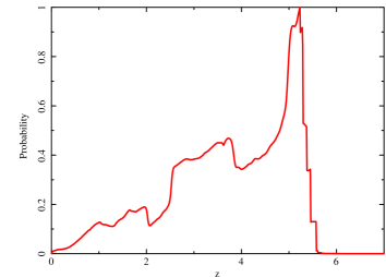
Figure 1: Probability density function corresponding to the photometric redshift determination of source 95 (Hsu et al. 2014).

We find that nine sources are highly absorbed with column densities above 10²³ cm^-2, eight of which are at the 90% confidence level. However, only three of these can be considered as CT AGN: sources 95, 230, and 309 (Chandra ids), although source 95 is only marginally CT. In the case of source 95, it is very surprising to be able to detect a near-CT AGN at redshift higher than 5. We examined the probability density function (PDF) for the photometric redshift in this case (Hsu et al. 2014). Although the PDF is somewhat flat towards lower redshifts, there is a clear peak at z = 5.22 (see Fig. 1). We also attempted to constrain the redshift value directly from X-ray spectral fitting. There seems to be an emission feature around 1.8 keV, although it is not very significant. Assuming that this feature is real and corresponds to the Fe K$\alpha$ emission line, we derived a z $\sim$ 2.8 and a resulting column density of a few times 10²³ cm^-2. Source 309 was already classified as a CT source in Feruglio et al. (2011). Here we also confirm its CT nature using XMM-Newton data. Although most CT AGN display a very strong Fe K$\alpha$ emission line, we were unable to detetect it in the case of source 230. However, CT AGN with very high column densities and modest Fe K$\alpha$ emission lines are not extremely rare, especially at high luminosities (L${}_{X}>$ 10⁴⁴ erg s^-1; see Fukazawa et al. 2011; Iwasawa et al. 2012). Finally, although most of the sources are obscured (N_H $>$ 10²² cm^-2, and $>$ 10²³ cm^-2 in most cases), we also found that two sources seem to be unabsorbed (sources 170 and 326).

Variability, and especially the lack of variability, has also been proposed as a method to pinpoint CT sources. As can be seen in Table 4, our CT candidates are among the less variable sources, however, our observations span many years and CT AGN have been shown to display variability in such long timescales.

Table 2: XMM-Newton and Chandra joint spectral fits

LID	z	$\rm N_{H}$	P1/P2	cstat/dof	EW	Flux	log LX	log LXunabs
		1022 cm-2			keV	$10^{-15}$ $\rm erg\,cm^{-2}\,s^{-1}$	$\rm erg\,s^{-1}$	$\rm erg\,s^{-1}$
(1)	(2)	(3)	(4)	(5)	(6)	(7)	(8	(9)
95	5.22	$81^{+20}_{-15}$	$<0.006$	2566/2427	$<0.4$	$1.9^{+2.3}_{-1.4}$	$43.6^{+0.4}_{-0.6}$	44.7
197	1.81	$44^{+30}_{-12}$	0.005	2103/3031	$0.20^{+0.07}_{-0.07}$	$0.74^{+0.27}_{-0.28}$	$42.63^{+0.13}_{-0.22}$	43.34
232	2.291	$15^{+2}_{-2}$	0.001	2917/3031	$0.13^{+0.08}_{-0.10}$	$5.3^{+0.3}_{-0.3}$	$43.97^{+0.02}_{-0.03}$	44.30
307	1.90	$19^{+6}_{-3}$	0.01	2018/2173	$0.34^{+0.19}_{-0.20}$	$1.44^{+0.14}_{-0.20}$	$43.20^{+0.05}_{-0.06}$	43.57
309	2.579	$580^{+550}_{-240}$	0.001	1548/1760	$1.0^{+0.25}_{-0.29}$	$1.5^{+0.3}_{-0.2}$	$42.75^{+0.05}_{-0.05}$	44.18
321	1.603	$1.70^{+0.14}_{-0.13}$	$<$0.0001	2509/2365	$<0.10$	$12.1^{+0.03}_{-0.03}$	$44.21^{+0.01}_{-0.01}$	44.25
346	1.221	$13^{+3}_{-2}$	0.02	2773/2667	$0.070^{+0.002}_{-0.002}$	$6.0^{+0.4}_{-0.5}$	$43.44^{+0.03}_{-0.03}$	43.69

• The columns are: (1) Chandra ID from the Luo et al. (2010) catalogue. (2) Redshift. (3) Intrinsic column density. (4) Ratio between the power-law normalizations in case of a double power-law model. (5) C-stat value to degrees of freedom ratio. (6) Fe K$\alpha$ rest-frame equivalent width. (7) Observed flux in the 2-10 keV band. (8) Observed luminosity in the 2-10 keV band. (9) Unabsorbed luminosity in the 2-10 keV band.

Table 3: Chandra spectral fits

LID z $$\rm N_{H}$$ P1/P2 cstat/dof EW Flux log L_X log L_Xunabs

10²² cm^-2 keV

(1) (2) (3) (4) (5) (6) (7) (8) (9)

117 1.51 0.02 392/390 43.41

170 1.22 93/117 41.50

199 2.45 0.02 162/205 43.52

230 2.61 0.001 119/135 44.82

293 3.88 0.002 195/228 1.0 43.31

326 3.10 211/287 43.45

397 2.28 0.04 309/324 43.56

• The columns are: (1) Chandra ID from the Luo et al. (2010) catalogue. (2) Redshift. (3) Intrinsic column density. (4) Ratio between the power-law normalizations in case of a double power-law model. (5) C-stat value to degrees of freedom ratio. (6) Fe K$\alpha$ rest-frame equivalent width. (7) Observed flux in the 2-10 keV band. (8) Observed luminosity in the 2-10 keV band. (9) Unabsorbed luminosity in the 2-10 keV band.

Table 4: Variability of X-ray detected DOGS.

LID Epochs Reduced $$\chi^{2}$$

95 4 0.38

117 4 3.31

170 2 -

197 4 1.13

199 4 0.99

230 3 0.15

232 4 9.35

293 4 0.68

307 4 0.31

309 4 0.64

321 4 25.72

326 4 1.09

346 4 3.36

397 4 1.87

• Results from $\chi^{2}$ fitting assuming a constant model.

$$\begin{array}[]{ccc}\includegraphics[angle={0},width=130.08731pt]{95_eufre.eps}&\includegraphics[angle={0},width=130.08731pt]{95_nh_cont.eps}&\includegraphics[angle={0},width=130.08731pt]{95_sed.eps}\\ \includegraphics[angle={0},width=130.08731pt]{117_eufre.eps}&\includegraphics[angle={0},width=130.08731pt]{117_nh_cont.eps}&\includegraphics[angle={0},width=130.08731pt]{117_sed.eps}\\ \includegraphics[angle={0},width=130.08731pt]{170_eufre.eps}&\includegraphics[angle={0},width=130.08731pt]{170_nh_cont.eps}&\includegraphics[angle={0},width=130.08731pt]{170_sed.eps}\\ \includegraphics[angle={0},width=130.08731pt]{197_eufre.eps}&\includegraphics[angle={0},width=130.08731pt]{197_nh_cont.eps}&\includegraphics[angle={0},width=130.08731pt]{197_sed.eps}\\ \includegraphics[angle={0},width=130.08731pt]{199_eufre.eps}&\includegraphics[angle={0},width=130.08731pt]{199_nh_cont.eps}&\includegraphics[angle={0},width=130.08731pt]{199_sed.eps}\\ \end{array}$$

Figure 2: Left: X-ray spectral fits (unfolded model and residuals) for the X-ray detected DOGs in our sample. Filled circles and empty squares correspond to Chandra and XMM-Newton data, respectively. Middle: Comparison between the confidence contours for the column density values computed for the 4 Ms data (dashed line) and 6 Ms data (solid line). The horizontal dotted line indicates the 90% confidence level. Right: SED fits for our X-ray DOGs sample. Solid line: full model; dotted line: AGN contribution; dash-dotted line: stellar contribution; and dashed line: starburst contribution. Our Compton-thick candidates are sources 95, 230, and 309.

$$\begin{array}[]{ccc}\includegraphics[angle={0},width=130.08731pt]{230_eufre.eps}&\includegraphics[angle={0},width=130.08731pt]{230_nh_cont.eps}&\includegraphics[angle={0},width=130.08731pt]{230_sed.eps}\\ \includegraphics[angle={0},width=130.08731pt]{232_eufre.eps}&\includegraphics[angle={0},width=130.08731pt]{232_nh_cont.eps}&\includegraphics[angle={0},width=130.08731pt]{232_sed.eps}\\ \includegraphics[angle={0},width=130.08731pt]{293_eufre.eps}&\includegraphics[angle={0},width=130.08731pt]{293_nh_cont.eps}&\includegraphics[angle={0},width=130.08731pt]{293_sed.eps}\\ \includegraphics[angle={0},width=130.08731pt]{307_eufre.eps}&\includegraphics[angle={0},width=130.08731pt]{307_nh_cont.eps}&\includegraphics[angle={0},width=130.08731pt]{307_sed.eps}\\ \includegraphics[angle={0},width=130.08731pt]{309_eufre.eps}&\includegraphics[angle={0},width=130.08731pt]{309_nh_cont.eps}&\includegraphics[angle={0},width=130.08731pt]{309_sed.eps}\\ \end{array}$$

Figure 2: Continued.

$$\begin{array}[]{ccc}\includegraphics[angle={0},width=130.08731pt]{321_eufre.eps}&\includegraphics[angle={0},width=130.08731pt]{321_nh_cont.eps}&\includegraphics[angle={0},width=130.08731pt]{321_sed.eps}\\ \includegraphics[angle={0},width=130.08731pt]{326_eufre.eps}&\includegraphics[angle={0},width=130.08731pt]{326_nh_cont.eps}&\includegraphics[angle={0},width=130.08731pt]{326_sed.eps}\\ \includegraphics[angle={0},width=130.08731pt]{346_eufre.eps}&\includegraphics[angle={0},width=130.08731pt]{346_nh_cont.eps}&\includegraphics[angle={0},width=130.08731pt]{346_sed.eps}\\ \includegraphics[angle={0},width=130.08731pt]{397_eufre.eps}&\includegraphics[angle={0},width=130.08731pt]{397_nh_cont.eps}&\includegraphics[angle={0},width=130.08731pt]{397_sed.eps}\\ \end{array}$$

Figure 2: Continued.

5 Spectral energy distributions

To obtain the AGN contribution to the IR emission in our sample, we took advantage of the multi-wavelength coverage of the CDF-S region to construct and fit the spectral energy distributions (SEDs) of our sources. There are enough multi-wavelength data for all of our 14 X-ray detected DOGs to obtain reliable SED fits, but there are only enough data for 34 of the X-ray undetected DOGs to carry out the same analysis.

We used the SEd Analysis with BAyesian Statistics (SEABASs; Rovilos et al. 2014) fitting code that combines SED templates and fit them using a maximum likelihood method with the posibility of including priors. We used three sets of templates to account for the stellar, starburst, and AGN contributions. The stellar templates are those from the library of synthetic templates of Bruzual & Charlot (2003). For the starburst templates we used two sets of libraries: those presented in Chary & Elbaz (2001), and Mullaney et al. (2011). For the AGN contribution, we used the library of Silva et al. (2004). In a small number of sources, the AGN contribution did not seem to be estimated properly, so we also included the AGN templates described in Polletta et al. (2007).

The IR luminosities obtained from the SED fitting are listed in Table 5 and Table 6, for the X-ray detected and the X-ray undetected DOGs, respectively. The L_IR derived from the SED fitting are not always over the 10¹² L$\odot$ value usually reported for DOGs, but they are over or very close to this value in the vast majority of cases. The resulting SEDs for the X-ray detected DOGs, showing each contribution separately, are plotted in the right panel of Fig, 2. We do not find any significant AGN contribution to the mid-IR emission in the two cases of sources 326 and 397, although the presence of an AGN is confirmed by their X-ray properties. Moreover, in four additional cases (sources 170, 197, 199, and 293), the AGN emission does not contribute significantly to the mid-IR luminosity. In the case of X-ray undetected DOGs, we do not find any AGN contribution in 16 cases (47% of the X-ray undetected DOGs with reliable SED fits). It is important to note that for 70% of the X-ray detected DOGs and 85% of the undetected DOGs with available SED fits, the derived L_12μm for the starburst component is larger than for the AGN component.

Table 5: Results from the SED fits for the X-ray detected DOGs.

LID z $$\rm logL_{IR}(8-1000\mu m)$$ log Stellar mass SFR

(1) (2) (3) (4) (5) (6) (7) (8) (9)

95 5.22 13.45 46.28 46.08 45.85 43.93 12.30 4029

117 1.51 11.47 44.38 44.04 44.12 41.96 9.87 37

170 1.22 11.51 44.09 44.08 42.16 41.96 10.91 56

197 1.81 12.11 44.82 44.82 42.59 42.42 11.11 220

199 2.45 12.38 45.09 45.08 41.97 42.75 11.34 410

230 2.61 12.50 44.96 44.87 44.23 42.82 11.51 525

232 2.291 12.39 45.34 44.91 45.13 42.85 10.76 272

293 3.88 13.55 46.26 46.26 42.74 42.30 10.95 6164

307 1.90 11.71 44.50 44.36 43.93 41.87 10.52 79

309 2.579 13.01 45.74 45.71 44.59 42.82 11.33 1722

321 1.603 12.22 45.33 44.34 45.28 42.69 10.93 75

326 3.10 12.66 45.37 45.37 - 42.70 11.35 790

346 1.221 11.87 44.78 44.41 44.54 41.49 9.21 90

397 2.28 11.94 44.65 44.65 - 42.65 11.17 150

• The columns are: (1) Chandra ID from the Luo et al. (2010) catalogue. (2) Redshift. (3) Total IR luminosity (8-1000 $\mu m$). (4) Total luminosiy at 12 $\mu$m. (5) Luminosity of the starburst component at 12 $\mu$m. (6) Luminosity of the AGN component at 12 $\mu$m. (7) Luminosity of the stellar component at 12 $\mu$m. (8) Stellar mass. (9) Star formation rate.

Table 6: Results from the SED fits for X-ray undetected DOGs with SED fitting

RA DEC z $$\rm logL_{IR}(8-1000\mu m)$$ log Stellar mass SFR

(1) (1) (2) (3) (4) (5) (6) (7) (8) (9)

53.0022 -27.7390 1.78 12.67 44.77 44.57 44.32 42.45 11.04 788

53.0050 -27.7768 1.90 12.94 45.01 44.52 44.83 42.94 11.63 1412

53.0203 -27.7798 1.04 11.52 44.28 44.28 - 42.39 11.35 58

53.0354 -27.6901 1.74 12.46 45.22 45.21 43.26 42.70 11.39 502

53.0365 -27.8875 1.95 12.59 44.93 44.13 44.86 42.49 11.18 569

53.0501 -27.8331 1.76 12.24 45.00 44.99 42.85 42.36 11.05 303

53.0602 -27.8761 2.17 12.15 44.91 44.90 - 42.61 11.30 249

53.0733 -27.7642 1.81 11.93 44.69 44.68 43.07 42.43 11.08 149

53.0772 -27.8595 2.88 12.92 45.68 45.68 - 43.12 11.77 1473

53.0860 -27.7095 1.97 12.07 44.83 44.82 42.90 42.67 10.58 206

53.0898 -27.9399 1.51 12.66 45.42 45.42 - 42.83 11.42 812

53.0965 -27.8518 1.65 11.65 44.41 44.40 42.67 42.20 10.89 78

53.0965 -27.6725 3.04 12.60 45.36 45.35 43.58 42.80 11.45 695

53.1215 -27.8214 2.70 12.40 45.16 45.15 42.96 42.54 11.23 442

53.1385 -27.6719 1.77 12.09 44.85 44.85 - 42.61 11.29 217

53.1552 -27.9485 2.19 12.46 44.47 44.05 44.26 42.26 10.61 473

53.1578 -27.7041 2.46 12.75 45.50 45.50 - 43.07 11.72 982

53.1598 -27.8502 2.03 12.14 44.90 44.90 - 42.45 11.11 244

53.1614 -27.6515 1.75 11.91 44.67 44.67 - 42.56 11.25 144

53.1636 -27.8907 2.87 12.81 45.74 45.42 45.46 42.86 11.45 817

53.1677 -27.8304 1.57 12.15 44.91 44.91 - 42.53 11.21 251

53.1736 -27.7227 1.93 11.96 44.72 44.71 - 42.48 11.17 160

53.1790 -27.6836 1.87 12.34 45.10 45.09 43.20 42.64 11.29 380

53.1868 -27.8316 2.10 11.99 44.75 44.74 42.86 42.50 11.16 170

53.1926 -27.8921 1.44 11.99 44.75 44.75 - 42.24 11.10 174

53.1949 -27.9490 1.72 11.84 44.60 44.59 43.15 42.20 10.11 120

53.1983 -27.7479 1.34 11.87 44.64 44.63 - 42.44 10.34 131

53.2131 -27.6718 1.93 11.84 44.60 44.58 43.24 42.50 10.73 119

53.2132 -27.6613 1.41 12.05 44.80 44.80 - 42.43 11.20 196

53.2170 -27.7635 1.59 11.98 44.73 44.73 - 42.66 11.34 168

53.2232 -27.7195 1.01 11.77 43.69 43.68 - 42.10 11.06 101

53.2234 -27.7151 1.78 12.50 44.52 44.09 44.32 42.38 10.61 518

53.2456 -27.9310 1.72 12.21 44.97 44.97 - 42.54 11.23 291

53.2611 -27.8583 2.14 11.87 44.64 44.62 43.27 42.30 10.95 130

• The columns are: (1) Optical coordinates (J200). (2) Redshift. (3) Total IR luminosity (8-1000 $\mu m$) (4) Total luminosiy at 12$\mu$m. (5) Luminosity of the Starburst component at 12$\mu$m. (6) Luminosity of the AGN component at 12$\mu$m. (7) Luminosity of the stellar component at 12$\mu$m. (8) Stellar masss. (9) Star formation rate.

6 Discussion

6.1 Relation between 12 $\mu m$ and 2-10 keV luminosities

A strong correlation has been found between mid-IR and X-ray emission in AGN (Krabbe et al. 2001, Gandhi et al. 2009, Levenson et al. 2009, Mateos et al. 2015, Stern 2015). This was expected since absorbed AGN emission would be re-processed and re-emitted in the IR. This correlation has been proposed as a possible selection technique for CT AGN. CT AGN, because of the strong supression of the X-ray continuum, should fall below this correlation if we plot the observed X-ray luminosity against their IR emission. However, it is difficult to isolate the AGN IR emission due to contamination by the galaxy starlight and the star formation IR emission.

We used the estimated AGN luminosity at 12 $\mu m$ from the SED fitting and the 2-10 keV observed luminosities from the X-ray spectral fits to see whether our sources follow the observed correlation (see Fig. 3). The shaded region in Fig. 3 corresponds to the relation presented in Gandhi et al. (2009). We also plotted the intrinsic 2-10 keV luminosity (open circles), i.e. corrected by the measured absorption. Although all our DOGs do not follow the correlation well, the three candidate CT AGN are clearly located towards the expected CT region, i.e. the region below the line that corresponds to a factor of 30 lower X-ray luminosity, as is typical in many CT AGN. It is important to point out that the relation presented in Gandhi et al. (2009) is based on high-spatial resolution data, whereas ours is derived from SED fitting, which could explain the deviations from the correlation in Gandhi et al. (2009) in our case.

Nine of the X-ray undetected DOGs lie in the CT region, however, for three of these (the three less luminous ones), the extremely low luminosities accompanied by rather high redshifts ($\langle$z$\rangle$ $\sim$ 1.8) do not strongly support a CT classification.

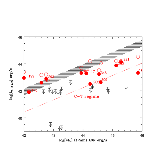
Figure 3: $\nu$L_ν12μm for the AGN component vs. L_2-10keV. Shaded region corresponds to Gandhi et al. 2009 relation. Filled and open circles correspond to observed and absorption-corrected L_X luminosities,for the X-ray detected DOGs, respectively. Arrows correspond to X-ray luminosity upper limits for the X-ray undetected DOGs.

6.2 Star formation rates

We took advantage of the SED decomposition we performed to study the star formation properties of our sample. In star-forming galaxies, the star formation rate (SFR) and stellar mass follow a relation called the main sequence (MS) (Daddi et al. 2007b; Elbaz et al. 2007; Whitaker et al. 2012; Behroozi et al. 2013; Speagle et al. 2014), which depends on the stellar mass and evolves with redshift. Outliers from this relation, such as local ULIRGs and some submm-selected galaxies (SMGs), are undergoing intense starbursts episodes that are probably driven by major mergers.

The stellar mass is an output parameter of our SED fitting. To obtain the SFR, we converted the IR luminosity (8 - 1000 $\mu m$) of the starburst component to SFR using the relation in Kennicutt (1998), which assumes Salpeter initial mass function. The resulting values are plotted in Fig. 4 along with the MS for star-forming galaxies at z=1, 3, and 5 from Speagle et al. (2014). Our DOGs occupy a wide region of the plot, as has also been found for the Herschel detected DOGs presented in Calanog et al. (2013), but we do not find significant differences between the CT candidates and the rest of the sample. Although our sample is too small, the most prominent characteristic of our three CT candidates is to be among the DOGs with the highest stellar masses. The average stellar mass and standard deviation for the X-ray detected DOGs are $\langle M\star\rangle=2.6\times 10^{11}M\odot$ and $\sigma=4.9\times 10^{11}M\odot$; whereas they are $\langle M\star\rangle=1.8\times 10^{11}M\odot$ and $\sigma=1.3\times 10^{11}M\odot$ for the X-ray undetected DOGs. Considering our three CT X-ray detected DOGs, and the six CT candidates among the X-ray undetected DOGs, the fraction of CT AGN with $\langle M\star\rangle>2\times 10^{11}M\odot$ is $\sim$ 33%, whereas it is only $\sim$ 12% at lower masses.

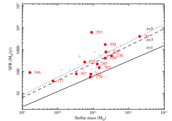
Figure 4: Stellar mass vs. SFR for the X-ray detected DOGS (filled circles), and X-ray undetected DOGs (crosses). The solid, dashed, and dotted lines correspond to the MS relation presented in Speagle et al. (2014) for z = 1, 3, and 5, respectively.

6.3 Previous X-ray spectral fits

The X-ray spectral fits were carried out in a different way in Georgantopoulos et al. (2011), so a direct comparison between the results is not possible. Eight sources from CDF-S in Georgantopoulos et al. (2011) were classified as possibly highly absorbed or CT AGN according to their flat photon index ($<1$) at high energies. All of these sources are highly absorbed (N_H $>$ 10²³ cm^-2) according to our spectral analysis, including two of our three CT candidates. Source 230, one of our CT candidates, was not flagged as possible CT in Georgantopoulos et al. (2011) because of the extremely small number of counts in its X-ray spectrum. For the remaining sources in Georgantopoulos et al. (2011) not considered as highly absorbed, we obtain column densities of the order of or lower than 10²² cm^-2.

We find only three possible CT candidates. The argument in favour of a big percentage of CT AGN among X-ray undetected DOGs comes mainly from the flat photon index in their stacked spectra. However, for 6 out of our 14 sources, we also find a very flat ($<$ 1.4) photon index if left free to vary, but we find only 3 CT candidates when computing the actual column densities. So it is possible, as suggested in Georgantopoulos et al. (2011), that the flat photon index in the stacked/averaged spectra could be the result of a mixture of a low fraction of CT sources combined with highly (but Compton-thin) absorbed sources. To test this hypothesis, we simulated a sample of AGN composed, similarly to the sample studied here of 20% CT AGN, 44% highly absorbed AGN, 22% moderately absorbed AGN, and 14% unabsorbed AGN. We then jointly fitted these simulated spectra, obtaining a photon index $\sim$ 1.1.

Brightman et al. (2014) presented X-ray spectral analysis for the 4 Ms Chandra spectra in the CDF-S. Our spectral fitting results are in agreement with those presented in Brightman et al. (2014) in most cases. In a few cases, there are small differences in the obtained column densities because of different photometric redshifts were used or because we used a more complex spectral model thanks to the availability of better spectral data. As for our three CT candidates, only source 309 is classified as such in Brightman et al. (2014). For the remaining two CT candidates in our sample (sources 95 and 230) and because of the limited number of counts, they only fitted the photon index for source 230 (obtaining a flat value $\sim$ 0.8) and all parameters were fixed in the case of source 95. In both cases, the column density was fixed to 10²⁰ cm^-2, i.e. they were classified as unabsorbed AGN. In any case, the location of these two sources in the L${}_{\rm 2-10\,keV}$/L_12μm plot supports their CT nature. In the case of source 170, Brightman et al. (2014) found it to be highly absorbed (almost CT), and we only found a low upper limit for the amount of absorption. Given the extremely low number of counts, a flat reflection dominated spectrum cannot be rejected in this case. Besides, the large uncertainty in its computed X-ray luminosity makes it consistent with the CT region.

6.4 Compton-thick/highly absorbed AGN fraction

Out of the 14 DOGs studied here, 9 sources have $N_{H}>10^{23}$ $\rm cm^{-2}\leavevmode\nobreak\$. If we compare the results in Georgantopoulos et al. (2011), which uses data from the CDF-N and CDF-S, with the results in Lanzuisi et al. (2009), it appears that despite the fact that the SWIRE sample is much brighter (its median flux is $\sim 1\times 10^{-13}$ $\rm erg\,cm^{-2}\,s^{-1}$ ), the percentage of highly absorbed sources ($>10^{23}$ $\rm cm^{-2}\leavevmode\nobreak\$) is not very different compared to our sample. However, when using the deeper data from this work (in which we only used data from the CDF-S), we find a higher percentage of highly absorbed sources ($\sim$ 64%) and a much higher percentage of CT sources ($\sim$ 20%).

In Fiore et al. (2009) they suggested that a higher percentage of CT sources could be hidden among the X-ray undetected DOGs given the very flat photon index obtained from stacked images. We also find that the spectra of our sources are flat but, after the spectral analysis, we find that the flat photon index comes from moderate to high absorption instead of from a high percentage of CT sources. To search for more CT candidates in our sample, we also attempted a join fit considering only the sources with spectroscopic redshifts available (only four sources), but the resulting best-fit model included only moderate amounts of absorption.

Our results could be consistent with the CT fraction estimated in Georgakakis et al. (2010) ($\sim$ 30%) as far as the X-ray detections are concerned. If we take into account the possibility that source 170 is a reflection-dominated CT AGN, as we mentioned in the previous section, our fraction of CT sources among X-ray detected DOGs would reach $\sim$ 30% as well.

Regarding the full DOGs sample, if we only consider the most secure CT AGN (the three candidates among the X-ray detected and the six candidates among the X-ray undetected DOGs), we estimate a fraction of 13% CT AGN among the whole DOGs population. If we assume that all the undetected DOGs without SED fitting available are CT candidates, this fraction would increase to 44%. However, strong star formation is also expected to produce a high $f_{24\mu m}$/f_R ratio by increasing the 24 $\mu m$ flux. As the AGN contribution becames stronger, it dominates the 24 $\mu m$ flux so that the fraction of AGN among DOGs increases for higher fluxes (Riguccini et al. 2015; Donley et al. 2012; Fiore et al. 2009; Dey et al. 2008). We examined the 24 $\mu m$ fluxes of the X-ray detected and undetected DOGs. Both samples display very high 24 $\mu m$ fluxes, although the X-ray detected DOGs show marginally higher fluxes (see Fig. 5). By applying a K-S test, we find that the probability that the two samples are drawn from the same population is high (p$\sim$0.5). Nevertheless, we find that 47% of the X-ray undetected DOGs with SED fits do not need any AGN contribution to their IR emission. Therefore, a significant percentage of the remaining X-ray undetected DOGs could be still be powered by star formation rather than by an AGN.

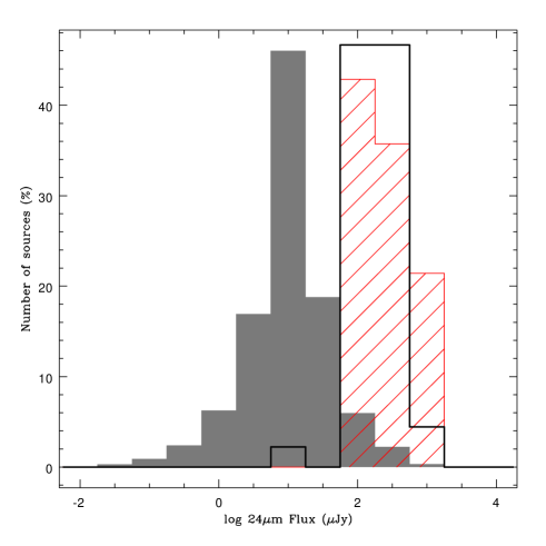
Figure 5: Distribution of 24 $\mu m$ fluxes for all the detected sources in the CDF-S (filled histogram), X-ray detected DOGs (line-shaded histogram), and X-ray undetected DOGs (empty histogram).

7 Conclusions

We have explored the properties of the X-ray detected and undetected DOGs in the CDF-S. This is an extension of the work presented in Georgantopoulos et al. (2011), but we had the advantages of not only the availability of deeper (6 Ms) Chandra observations of the sources presented in Georgantopoulos et al. (2011), but also the addition of deep (3 Ms) XMM-Newton observations in the CDF-S. We also present a more accurate estimate of the AGN contribution to the IR luminosity by SED fitting from the UV to the far-IR. Out of the 70 DOGs composing the full sample, 14 are X-ray detected. For the remaining 56 DOGs, there were enough multi-wavelength data available for 34 of these DOGs to perform a similar SED-fitting based analysis as for the X-ray detected sources.

From the X-ray spectral analysis, we find that most (9/14) of the X-ray detected DOGs in our sample show high obscuration (N_H $>10^{23}$ $\rm cm^{-2}\leavevmode\nobreak\$). However, only three (maybe four) of our X-ray detected DOGs could be CT AGN, so we estimate a CT fraction of 20-30 % among X-ray detected DOGs. Many of our DOGs (6/14) show flat photon indices ($\Gamma$ $\lesssim$ 1.4), but only three display CT absorption. Therefore, caution must be exercised when estimating the fraction of CT AGN from the photon index of stacked/averaged spectra.

Considering the full DOGs sample, the fraction of CT AGN among the whole DOGs population could range from 13 to 44%. X-ray detected DOGS seem to have marginally higher 24 $\mu m$ fluxes and CT X-ray detected DOGs seem be hosted in galaxies with higher stellar masses than X-ray undetected DOGs, but a bigger sample is necessary to confirm these results.