Two-dimensional Fröhlich interaction in transition-metal-dichalcogenide monolayers: theoretical modeling and first-principles calculations

Abstract

We perform ab initio calculations of the coupling between electrons and small-momentum polar-optical phonons in monolayer transition metal dichalcogenides of the 2H type: MoS₂, MoSe₂, MoTe₂, WS₂, and WSe₂. The polar-optical coupling with longitudinal optical phonons, or Fröhlich interaction, is fundamentally affected by the dimensionality of the system. In a plane-wave framework with periodic boundary conditions, the Fröhlich interaction is affected by the spurious interaction between the 2D material and its periodic images. To overcome this difficulty, we perform density functional perturbation theory calculations with a truncated Coulomb interaction in the direction perpendicular to the plane of the 2D material. We show that the two-dimensional Fröhlich interaction is much stronger than assumed in previous ab initio studies. We provide analytical models depending on the effective charges and dielectric properties of the materials to interpret our ab initio calculations. Screening is shown to play a fundamental role in the phonon-momentum dependency of the polar-optical coupling, with a crossover between two regimes depending on the dielectric properties of the material relative to its environment. The Fröhlich interaction is screened by the dielectric environment in the limit of small phonon momenta and sharply decreases due to stronger screening by the monolayer at finite momenta. The small-momentum regime of the ab initio Fröhlich interaction is reproduced by a simple analytical model, for which we provide the necessary parameters. At larger momenta, however, direct ab initio calculations of electron-phonon interactions are necessary to capture band-specific effects. We compute and compare the carrier relaxation times associated to the scattering by both LO and A₁ phonon modes. While both modes are capable of relaxing carriers on timescales under the picosecond at room temperature, their absolute and relative importance vary strongly depending on the material, the band, and the substrate.

I Introduction

Among the rapidly expanding family of two-dimensional (2D) materials, monolayer transition metal dichalcogenides (TMDs) offer particularly interesting features for electronic and optoelectronic applicationsRadisavljevic et al. (2011); Wang et al. (2012); Jariwala et al. (2014); Ganatra and Zhang (2014); Fiori et al. (2014). Thanks to high carrier mobility and a direct band gap in the visible range they can be included in 2D van der Waals heterostructures to fulfil various functionalities associated to light-matter interaction and electron transport. In this context, it is essential to reach a good understanding of carrier scatteringMoody et al. (2015); Wang et al. (2015); Shi et al. (2013), including the intrinsic contribution from the electron-phonon interaction. In TMDs and other polar materials, a peculiar coupling emerges between electrons and longitudinal optical (LO) phonons. Such polar phonons interact with electrons by inducing a polarization density. At small phonon momenta, this polar-optical coupling, or Fröhlich interaction, can become quite large compared to standard electron-phonon coupling (EPC). Dimensionality has an interestingly drastic effect on this interaction. Indeed, in the limit of zero phonon momentum, the Fröhlich interaction diverges in a material with three-dimensional (3D) periodicity while it tends to a finite value in 2D materials. This effect can be traced back to the behaviour of the long-range Coulomb interaction.

Density functional perturbation theoryBaroni et al. (2001) (DFPT) is a powerful tool to simulate electron-phonon interactions. Associated to analytical modelsVogl (1976); Sarma and Mason (1985); Mori and Ando (1989), this method can be used to establish quantitative modelsSjakste et al. (2015) of the Fröhlich interaction in bulk materials. Such a comprehensive and quantitative study of the Fröhlich interaction is still missing in the case of 2D materials. This is mainly due to the limitations of DFPT in the 2D framework. Indeed, DFPT relies on 3D periodic boundary conditions, implying the presence of periodic images when simulating low-dimensional systems. Since long-range Coulomb interactions between periodic images arise when low-dimensional systems are perturbed at small momentaSohier et al. (2015), DFPT fails to account for the peculiarities of the Fröhlich interaction in 2D. In addition to those computational limitations, deriving analytical models of the Fröhlich interaction is not straightforward. In particular, the screening of the Coulomb interaction in 2D materials is a complex mechanismKeldysh (1979); Cudazzo et al. (2011); Wehling et al. (2011); Berkelbach et al. (2013); Steinhoff et al. (2014) requiring careful modeling.

In a previous ab initio studyKaasbjerg et al. (2012) of EPC in MoS₂, the small-momentum behaviour of the 2D Fröhlich interaction was estimated by fitting a 2D analytical model on ab initio calculations. However, the calculations were performed at momenta too large to capture the effects of dimensionality and the analytical model only partially accounted for the complex screening occurring in 2D materials. The 2D Fröhlich interaction was found to participate only moderately to the coupling with optical phonons in MoS₂, with a small-momentum limit three times smaller than the value reported here. Consequently, it was often ignored in following ab initio studies of EPC in TMDsLi et al. (2013); Jin et al. (2014). As far as modeling of the interaction is concerned, a more sophisticated modelKeldysh (1979); Cudazzo et al. (2011); Wehling et al. (2011); Berkelbach et al. (2013); Steinhoff et al. (2014) of screening in 2D materials was used to estimate the strength of the Fröhlich interaction in a recent workDanovich et al. (2015). This was done in the case of an isotropic dielectric tensor for the monolayer and without the support of direct ab initio computation of electron-phonon interactions.

We recently implementedSohier (2015) the truncation of the Coulomb interaction between periodic images of 2D materials in the DFT and DFPT package Quantum ESPRESSOGiannozzi et al. (2009) (QE). This technique enables us to isolate each slab and simulate electron-phonon interactions in a 2D framework. In this work we use this approach to compute the 2D Fröhlich interaction from first principles. We focus on the 2H polytypes of MoS₂, MoSe₂, MoTe₂, WS₂, and WSe₂. We propose developments on the analytical model of the Fröhlich interaction in 2D, especially concerning its screening in the case of a monolayer with anisotropic dielectric properties and for different dielectric environment on each side of the monolayer. We use ab initio calculations to estimate the parameters of this analytical model. The analytical model is used to interpret and support our calculations of the coupling to LO phonons, and a simple effective model is proposed to reproduce its small-momentum limit. The analytical model is also used to estimate the effect of the presence of a substrate on the Fröhlich interaction. Finally, we compute the inverse relaxation times associated to intraband scattering of carriers by LO and A₁ phonons. Large variations are observed from material to material. The relative importance of the LO and A₁ contributions strongly depends on the band in which we consider such scattering. In any case, optical phonons (LO and/or A₁) are shown to be capable of relaxing carriers on a time scale inferior to the picosecond at room temperature.

II ab initio simulations of electron-phonon coupling

We perform DFPT calculations of EPC in monolayer TMDs (2H type), using our recently developed 2D Coulomb cutoff approachSohier (2015) within the Quantum ESPRESSOGiannozzi et al. (2009) (QE) distribution. This approach consists in truncating the Coulomb interaction between the periodic images of the 2D material. This was implemented for the computation of total energy, forces, phonons and electron-phonon coupling. The technique requires the periodic images to be separated by at least twice the thickness of the electronic density of the simulated layer. We use a separation of $\approx 17$ Å, largely fulfilling that requirement. Within a slab of thickness $\approx 12$ Å  everything happens as if the monolayer was isolated. Further details about the implementation of the 2D Coulomb cutoff in the DFT and DFPT packages of the QE distribution method will be exposed in a separate publication. We use pseudopotentials from the Standard Solid-State Pseudopotentials (SSSP) library (accuracy version) with PBE functionals and kinetic energy cutoff as indicated in the library. Spin-orbit coupling is neglected. Starting from experimental lattice parametersPodberezskaya et al. (2001), structures are relaxed to minimize the total energy in our DFT framework. The resulting in-plane lattice parameters $a_{0}$, subsequently used in our calculations, are given in Table 4. The electronic-momentum grid is set to $16\times 16\times 1$. Those choices are sufficient to obtain optical phonon energies within a few cm^-1 of experimental values (when available).

In this section, MoS₂ is used as an example. We perform calculations in bulk MoS₂ as well to highlight the impact of dimensionality on the Fröhlich interaction. For bulk MoS₂, we use the standard QE distribution and the experimentalPodberezskaya et al. (2001) out-of-plane lattice parameter of $c=12.29$ Å. The corresponding unit-cell includes two layers such that the interlayer distance in the bulk is $\approx 6.15$ Å. Note that a rigorous study of the bulk requires the inclusion of dispersion correctionsBrumme et al. (2015) to account for van der Waals interactions between layers. Since we only seek a comparison of the small-momentum behaviour of the Fröhlich interaction, however, we will ignore this aspect.

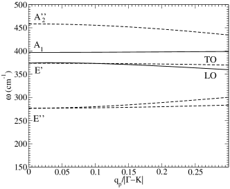
Figure 1: Dispersion of the optical phonons in monolayer MoS₂ at small momenta. For the modes in dashed lines, EPC matrix elements are negligible. The A₁ and LO modes, in plain lines, couple to electrons. We follow the notation of Ref. Molina-Sánchez and Wirtz, 2011  for the symmetry representations of the modes at $\mathbf{\Gamma}$. The E’ mode separates into LO and TO modes.

We note $\mathbf{e}_{\mathbf{q}_{p}\nu}$ and $\hbar\omega_{\mathbf{q}_{p}\nu}$ the eigenvector and energy associated to a phonon in branch $\nu$ with in-plane momentum $\mathbf{q}_{p}$. The dispersions of small-momentum optical phonons in MoS₂ are shown in Fig. 1. Among those, only the A₁ and LO modes (plain lines in Fig. 1) couple to electrons. In the small-momentum limit, the A₁ mode corresponds to out-of-plane displacements of the sulfur atoms in phase opposition while the molybdenum atoms are static. The LO mode corresponds to in-plane longitudinal displacements with the molybdenum atom moving in phase opposition to both sulfur atoms. A more extensive ab initio study of phonons in MoS₂ and WS₂ can be found in Ref. Molina-Sánchez and Wirtz, 2011. Optical phonon modes at small momenta are qualitatively similar for all the TMDs studied in this work.

We consider phonon-scattering of an electron from state $|\mathbf{k}\rangle$ to $|\mathbf{k}+\mathbf{q}\rangle$ within a given band. The associated EPC matrix element is defined as:

$$g_{\nu}(\mathbf{q}_{p}) =\sum_{a,i}\textstyle\sqrt{\frac{\hbar}{2M_{a}\omega_{\mathbf{q},\nu}}}\mathbf{e}^{a,i}_{\mathbf{q}_{p},\nu}\langle\mathbf{k+q}|\Delta^{a,i}_{\mathbf{q}_{p}}\mathcal{V}_{\rm{KS}}(\mathbf{r})|\mathbf{k}\rangle,$$ (1)

where $M_{a}$ is the mass of atom $a$ and $\Delta^{a,i}_{\mathbf{q}_{p}}\mathcal{V}_{\rm{KS}}(\mathbf{r})$ is the lattice periodic part of the derivative of the self-consistent Kohn-Sham potential with respect to a phonon displacement of atom $a$ in direction $i$.

We consider neutral TMDs to avoid the metallic nature of the electronic screening that would occur in doped layers. Our primary goal is the study of the long-range Fröhlich interaction, involving LO phonons at small momenta ($|\mathbf{q}_{p}|<15\%$ of $|\mathbf{\Gamma-K}|$) and an excited electron or hole. Considering the small-momenta restriction and the energy of LO phonons, we can focus on intraband scattering. We further narrow the study to the highest part of the valence band around the high-symmetry points $\mathbf{K}$ and $\mathbf{\Gamma}$, and the lowest part of the conduction band around $\mathbf{K}$. More precisely, we compute the EPC matrix elements $g_{\rm{LO}}(\mathbf{q}_{p})$ for the following pairs of electronic states : (i) $\mathbf{k}=\mathbf{K}-\mathbf{q}_{p}/2$ and $\mathbf{k}+\mathbf{q}_{p}=\mathbf{K}+\mathbf{q}_{p}/2$ in the conduction band, noted ”K cond” ; (ii) $\mathbf{k}=\mathbf{K}-\mathbf{q}_{p}/2$ and $\mathbf{k}+\mathbf{q}_{p}=\mathbf{K}+\mathbf{q}_{p}/2$ in the valence band, noted ” K val” ; (iii) $\mathbf{k}=\mathbf{\Gamma}-\mathbf{q}_{p}/2$ and $\mathbf{k}+\mathbf{q}_{p}=\mathbf{\Gamma}+\mathbf{q}_{p}/2$ in the valence band, noted ”$\Gamma$ val”. Momentum $\mathbf{q}_{p}$ is in the $\mathbf{\Gamma}\to\mathbf{M}$ direction to minimize LO/TO mixing.

The results of the calculations for MoS₂ are presented in Fig. 2. For comparison, we add the coupling $g_{\rm{A}_{1}}(\mathbf{q}_{p})$ associated to the other significant contribution of the A₁ mode. We recover the characteristic behaviours of the 2D and 3D Fröhlich interactions. In the 3D case, the interaction diverges as $\mathbf{q}_{p}\to\mathbf{\Gamma}$. In the 2D framework provided by our approach, however, the Fröhlich interaction tends to a constant at $\mathbf{\Gamma}$. Note that a divergence will occur when using the standard QE code, even if the interlayer distance is increased. The fact that we recover the finite limit of the coupling at $\mathbf{\Gamma}$ thus confirms that the truncation of the Coulomb interaction in QE is equivalent to simulating an isolated monolayer. The coupling to LO phonons at large momenta depends on the bands via the details of the electronic wave functions. Indeed, in that case, the variations of the polarization potential on the length scale of the width of the electronic states becomes relevant. Similar calculations were performed for monolayers of MoSe₂, MoTe₂, WS₂, and WSe₂, see Fig. 8 of the Appendix.

In Figs. 2 and 8, the plain lines represent analytical models discussed in the following sections. In those models, we will focus on the more general small-momentum behaviour of the Fröhlich interaction, which depends solely on the Born effective charges and dielectric properties of the material. From a modeling point of view, the existence of finite limit at $\mathbf{\Gamma}$ for the 2D interaction is easily established by considering the $1/|\mathbf{q}_{p}|$ dependence of the 2D Coulomb interaction in reciprocal space. The sharp decreasing of the coupling at finite-q, however, is a more subtle screening effect that remains to be studied in details. Our numerical DFPT method provide us with a support to treat this issue in a systematic manner and establish a quantitatively accurate analytical model.

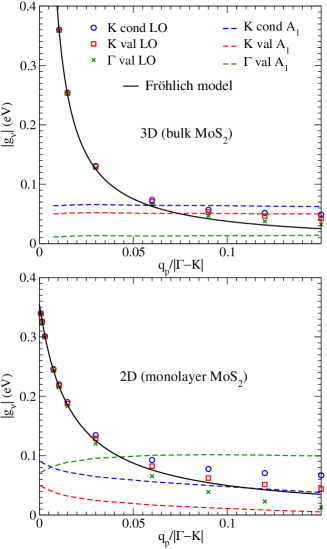
Figure 2: EPC matrix elements involving LO and A₁ phonon modes in bulk and monolayer MoS₂. We consider intraband scattering of electrons or holes in the conduction band near $\mathbf{K}$ (”K cond”)  and in the valence band near $\mathbf{K}$ and $\mathbf{\Gamma}$ (”K val” and ”$\mathbf{\Gamma}$ val”, respectively). Momenta $\mathbf{q}_{p}$ are in the $\mathbf{\Gamma}\to\mathbf{M}$ direction. The coupling to the LO phonons includes the Fröhlich interaction. The models for three-dimensional and two-dimensional Fröhlich interactions in bulk and monolayer MoS2 are represented in plain lines and described in the text. Dashed lines and symbols are DFPT calculations. The standard QE package was used for the bulk, while we used our implementation of the Coulomb cutoff in for the monolayer.

III Analytical Models of the Fröhlich interaction

We now present analytical models to explain our DFPT calculations and gain better understanding on the effect of dimensionality on the small-momentum limit of the Fröhlich interaction. The tensors of Born effective charges are noted $\mathcal{Z}^{b}_{a}$ and $\mathcal{Z}^{m}_{a}$ for bulk and monolayer, respectively. The index $a$ runs over the atoms of the unit cell. The relative dielectric permittivity tensors (simply called dielectric tensors hereafter) for bulk and monolayer are noted $\mathcal{E}^{b}$ and $\mathcal{E}^{m}$, respectively. By symmetry, the tensors are isotropic in the plane, but we allow for different properties in the out-of-plane direction. The tensors thus have the following generic forms:

$$\mathcal{E}=\begin{pmatrix}\epsilon_{p}&0&0\\ 0&\epsilon_{p}&0\\ 0&0&\epsilon_{z}\end{pmatrix}\ \ \ \mathcal{Z}_{a}=\begin{pmatrix}Z_{a,p}&0&0\\ 0&Z_{a,p}&0\\ 0&0&Z_{a,z}\end{pmatrix}.$$ (2)

In-plane and out-of-plane variables are separated according to the notation $\mathbf{r}\to(\mathbf{r}_{p},z)$ and $\mathbf{q}\to(\mathbf{q}_{p},q_{z})$. We use Gaussian CGS units.

III.1 Three-Dimensional bulk

We quickly recall the well-known results of the 3D case. The small momentum behaviour of the Fröhlich interaction is well described by the leading order in Vogl’s model Vogl (1976)

$$|g^{\rm{3D}}_{\rm{Fr}}(\mathbf{q}_{p})| =\frac{4\pi e^{2}}{V|\mathbf{q}_{p}|\epsilon^{b}_{p}}\sum_{a}\frac{\mathbf{e}_{\mathbf{q}_{p}}\cdot\mathcal{Z}_{a}^{b}\cdot\mathbf{e}^{a}_{\mathbf{q}_{p}\rm{LO}}}{\sqrt{2M_{a}\omega_{\mathbf{q}_{p}\rm{LO}}}},$$ (3)

where $e$ is the elementary charge, $V$ is the unit-cell’s volume, $\epsilon^{b}_{p}$ is the in-plane dielectric constant of the bulk ($15.37$ in MoS₂), and $\mathbf{e}_{\mathbf{q}_{p}}=\mathbf{q}_{p}/|\mathbf{q}_{p}|$. The pre-factor of $1/|\mathbf{q}_{p}|$ is essentially constant in the range of momenta considered in this work. A small dependency on norm and direction of $\mathbf{q}_{p}$ appears as the phonon modes deviate from the strictly longitudinal modes. This model is sufficient to reproduce the small-momentum limit of the Fröhlich interaction, as shown in Fig. 2 where the plain line is the above model.

III.2 Two-dimensional monolayer

Our objective is to derive the Fröhlich interaction in the system of Fig. 3. We consider LO phonons in a 2D material of thickness $t$. Its dielectric tensor $\mathcal{E}^{m}$ has the form of Eq. 2, with in-plane and out-of-plane dielectric constants $\epsilon^{m}_{p}$ and $\epsilon^{m}_{z}$, respectively. Above and below are two semi-infinite spaces with isotropic dielectric properties represented by the dielectric constants $\epsilon_{2}$ and $\epsilon_{1}$, respectively.

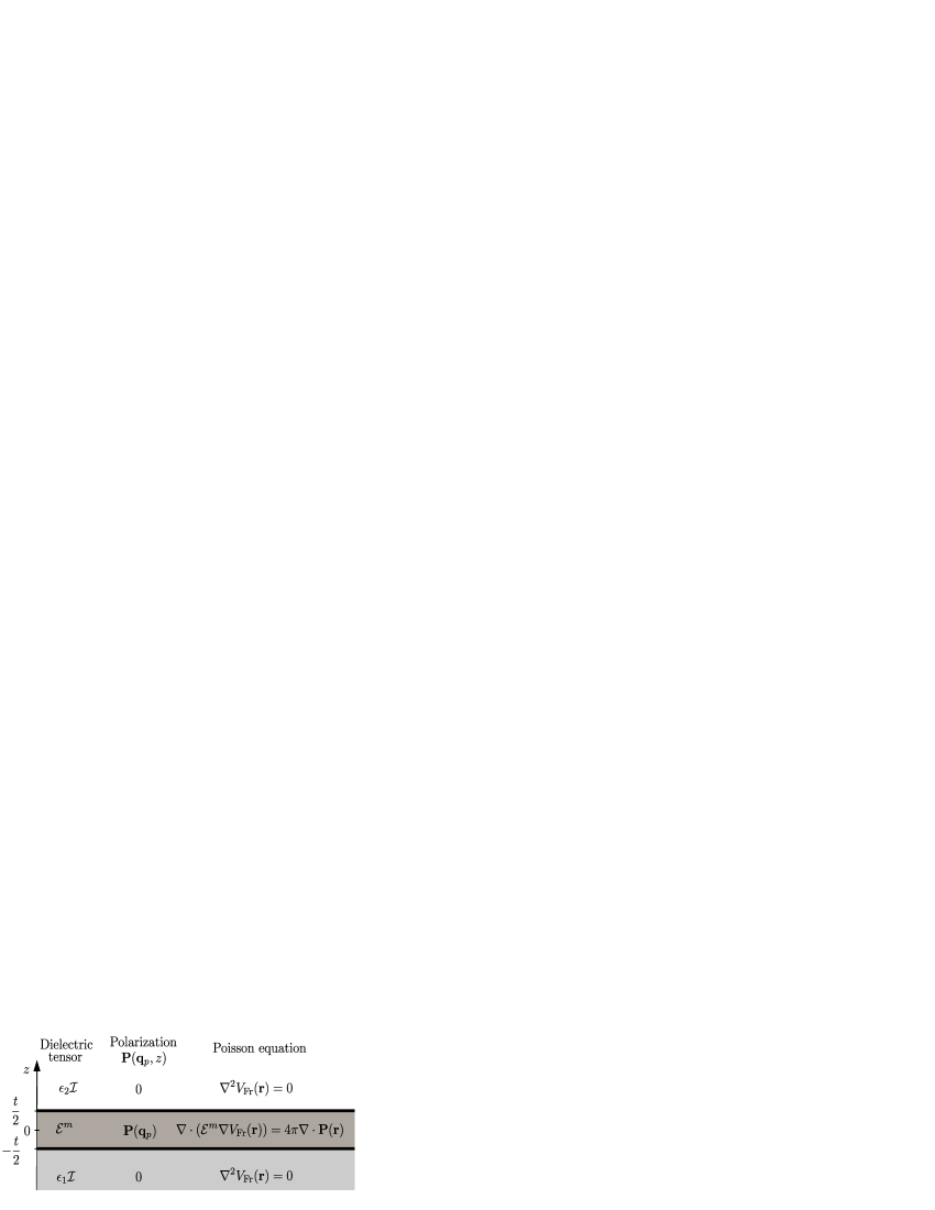
Figure 3: Model of the Fröhlich interaction in a polar 2D material of thickness t. LO phonons generate a periodic polarization density $\mathbf{P}(\mathbf{r}_{p},z)=\mathbf{P}(\mathbf{q}_{p},z)e^{i\mathbf{q}_{p}\cdot\mathbf{r}_{p}}$ inside the 2D material. The dielectric properties of the 2D material are represented by the dielectric tensor $\mathcal{E}^{m}$ with in-plane and out-of-plane dielectric constants $\epsilon^{m}_{p}$ and $\epsilon^{m}_{z}$, respectively. Above and below are two half spaces in which the polarization is zero and the dielectric constants are $\epsilon_{2}$ and $\epsilon_{1}$ respectively. The symbol $\mathcal{I}$ denotes the identity matrix. The two thick horizontal black lines represent surface charges at the interfaces of the 2D material due to the abrupt variations in the polarization density. We write the Poisson equation defining the Fröhlich potential $V_{\rm{Fr}}$ in each region.

The origin of the polar-optical coupling is the polarization density $\mathbf{P}(\mathbf{r}_{p},z)$ generated by the atomic displacement pattern associated to a LO phonon of in-plane momentum $\mathbf{q}_{p}$

$$\mathbf{P}(\mathbf{r}_{p},z)=\frac{e^{2}}{A}\sum_{a}\frac{\mathcal{Z}^{m}_{a}\cdot\mathbf{e}^{a}_{\mathbf{q}_{p}\rm{LO}}}{\sqrt{2M_{a}\omega_{\mathbf{q}_{p}\rm{LO}}}}f(z)\ e^{i\mathbf{q}_{p}\cdot\mathbf{r}_{p}},$$ (4)

where $A$ is the area of the unit-cell and $f(z)$ is the out-of-plane profile of the polarization (normalized to unity). Such a polarization density induces a potential $V_{\rm{Fr}}(\mathbf{r}_{p},z)=V_{\rm{Fr}}(\mathbf{q}_{p},z)e^{i\mathbf{q}_{p}\cdot\mathbf{r}_{p}}$ with the same periodicity. The associated EPC can then be written as

$$g^{\rm{2D}}_{\rm{Fr}}(\mathbf{q}_{p})=\int V_{\rm{Fr}}(\mathbf{q}_{p},z)n_{el}(z)dz,$$ (5)

where $n_{el}(z)$ is the plane-averaged electronic density. By using this expression, we neglect the details of the wave-functions and the associated band-dependency. In the out-of-plane direction, we will consider the electronic density and the polarization to be uniform over the thickness $t$ of the material

$$f(z)=n_{el}(z)=\frac{\theta{(t/2-|z|)}}{t},$$ (6)

where $\theta$ is the Heavyside function. This approximation should be satisfactory in the long wavelength limit, since $V_{\rm{Fr}}(\mathbf{q}_{p},z)$ varies mildly in the out-of-plane direction.

The potential $V_{\rm{Fr}}$ must fulfil the Poisson equation

$$\nabla\cdot(\mathcal{E}(z)\nabla V_{\rm{Fr}}(\mathbf{r})) =4\pi\nabla\cdot\mathbf{P}(\mathbf{r}),$$ (7)

where $\mathcal{E}(z)$ is a position dependent dielectric tensor. The central objects of the problem are the phonon-induced polarization density and the dielectric tensor. As one travels along the out-of-plane direction, both those quantities change. Inside the 2D material, $\mathcal{E}(z)=\mathcal{E}^{m}$ and the polarization density is finite and oscillating in the plane. Outside the 2D material, $\mathcal{E}(z)=\epsilon_{1}\mathcal{I}$ or $\epsilon_{2}\mathcal{I}$ (where $\mathcal{I}$ is the identity matrix) and the polarization density is zero. Other requirements on the potential are that that the associated in-plane electric field $\mathbf{E}^{\parallel}(\mathbf{r})$ and out-of-plane electric displacement $\mathbf{D}^{\perp}(\mathbf{r})$ should be continuous.

The detailed derivation of the solution to this model can be found in App. A. To allow for a more direct interpretation of the final solution in Eq. 36, we seek a more transparent form. By Taylor expansion of the denominator at the linear order in $|\mathbf{q}_{p}|$, the full expression of Eq. 36 can be recast in the form

$$\begin{split}|g^{\rm{2D}}_{\rm{Fr}}(\mathbf{q}_{p})|&=\frac{C_{\mathcal{Z}}}{\epsilon_{\rm{eff}}(|\mathbf{q}_{p}|)}\\ \epsilon_{\rm{eff}}(|\mathbf{q}_{p}|)&\approx\epsilon^{0}_{\rm{eff}}+r_{\rm{eff}}|\mathbf{q}_{p}|,\end{split}$$ (8)

where the expressions of the parameters are given in table 1. The above form is found to reproduce Eq. 36 very accurately. Only when $\epsilon^{m}_{z}\approx\epsilon_{1}$ or $\epsilon_{2}$ should one retain Eq. 36 rather than use Eq. 8. More quantitative results, depending on the nature of the monolayer, will be given in Sec. V. For now, let us make some qualitative remarks valid as long as the material is a stronger dielectric as the environment, which is the case of the monolayer TMDs discussed in this work, in vacuum or on SiO₂. The bare magnitude of the polar-optical coupling is given by $C_{\mathcal{Z}}$. The origin of the sharp decrease at finite $\mathbf{q}_{p}$ is a screening effect specific to 2D materials. It can be associated with the formation of surface charges due to the change in dielectric properties at the interfaces between the 2D material and its environment. The screening is characterized by the parameter $r_{\rm{eff}}$ which depends on the dielectric properties of the material as well as its thickness. Homogeneous to a distance, it can be interpreted as an effective thickness marking the crossover between two screening regimes. For $|\mathbf{q}_{p}|<<r^{-1}_{\rm{eff}}\epsilon^{0}_{\rm{eff}}$, the coupling is screened by $\epsilon^{0}_{\rm{eff}}$, which depends mainly on the dielectric properties of the environment. For $|\mathbf{q}_{p}|>>r^{-1}_{\rm{eff}}\epsilon^{0}_{\rm{eff}}$, the field lines are confined to the material, and the coupling is screened by the material. Materials with large dielectric constants (with respect to the environment) will tend to focus the field lines more strongly, which results in a larger effective thickness $r_{\rm{eff}}$ and a sharper decrease in the Fröhlich interaction at finite momenta (note that the slope of the coupling at $\mathbf{\Gamma}$ is proportional to $-r_{\rm{eff}}$).

Table 1: Full expressions of the parameters involved in the model of the 2D Fröhlich interaction, Eq. 8. See Fig. 3 and Eq. 2 for the definitions of the various parameters in the model. Note that for the isolated TMDs considered in our ab initio calculations, we have $\epsilon_{1}=\epsilon_{2}=\epsilon_{12}=1$, $\epsilon^{m}_{z}>>1$, and $\epsilon^{m}_{p}>>1$, which leads to $F\approx 1$, $\epsilon^{0}_{\rm{eff}}\approx 1$, and $r_{\rm{eff}}\approx\frac{\epsilon^{m}_{p}t}{2}$.

$C_{\mathcal{Z}}$ =	$\frac{2\pi e^{2}}{A}\sum_{a}\frac{\mathbf{e}_{\mathbf{q}_{p}}\cdot\mathcal{Z}_{a}^{m}\cdot\mathbf{e}^{a}_{\mathbf{q}_{p}\rm{LO}}}{\sqrt{2M_{a}\omega_{\mathbf{q}_{p}\rm{LO}}}}$
$\epsilon^{0}_{\rm{eff}}$ =	$\epsilon_{12}\frac{\epsilon^{m}_{z}\bar{\epsilon}}{\epsilon^{m}_{z}\bar{\epsilon}+\epsilon_{12}(\epsilon^{m}_{z}-\bar{\epsilon})}$
$r_{\rm{eff}}$ =	$\frac{(\epsilon^{0}_{\rm{eff}})^{2}}{\epsilon_{12}}\left(\frac{\epsilon_{12}}{3\epsilon^{m}_{z}}+\frac{\epsilon^{m}_{p}}{2\epsilon_{12}}F\right)\times t$
$F$ =	$1+\frac{\epsilon_{1}\epsilon_{2}}{\bar{\epsilon}^{2}}+\frac{\epsilon_{12}}{\bar{\epsilon}}-\frac{\epsilon^{2}_{12}}{\bar{\epsilon}\epsilon^{m}_{z}}-\frac{\epsilon^{2}_{12}}{\bar{\epsilon}^{2}}-\frac{\epsilon_{12}}{\epsilon^{m}_{z}}$
$\epsilon_{12}$ =	$\frac{\epsilon_{1}+\epsilon_{2}}{2}$       $\bar{\epsilon}\ =\ \sqrt{\epsilon^{m}_{z}\epsilon^{m}_{p}}$

We have derived the general expression for an anisotropic slab and different dielectric media above and below. It can be applied to any polar material. To be quantitatively predictive, we need to evaluate the parameters involved. We now detail how to evaluate those parameters with ab initio calculations.

IV ab initio Parameters

Here again, MoS₂ will be used as an example to illustrate the method. The final parameters of interest will then be given for the other TMDs. The parameters of the model are the Born effective charges, dielectric tensors and phonon eigenvectors. The dynamical matrix and the corresponding phonon eigenvectors are available from the electron-phonon calculations. The QE code computes clamped-ions dielectric tensors and Born effective charges by means of linear response calculations with respect to an electric field perturbationBaroni et al. (2001). The Born effective charges are related to the derivative of the forces on the atoms with respect to the applied electric field. Since our implementation of the 2D Coulomb cutoff includes the computation of forces, the Born effective charges can be computed in the 2D framework for the monolayers. Note, however, that equivalent results can be obtained with the standard code. Indeed, Born effective charges converge relatively fast towards their 2D values with respect to the distance between periodic images. The dielectric constant, on the other hand, is computed as a macroscopic quantity defined over a three-dimensional supercell. As such, the computation of the dielectric tensor of the bulk $\mathcal{E}^{b}$ is straightforward and reported in Table 2 for MoS2. The computation of an equivalent quantity relevant for 2D materials, however, raises issues beyond periodic images interactions Tóbik and Dal Corso (2004); Yu et al. (2008). As of yet, we did not implement the modifications necessary to compute dielectric tensors in a 2D framework. In the following, the dielectric tensors of the monolayers will be evaluated using the standard QE code, with an effort to extract relevant 2D quantities from 3D calculations.

The constant $C_{\mathcal{Z}}$ corresponds to the magnitude of the bare Fröhlich interaction. It depends on the Born effective charges and the phonon displacements. The components of the tensors $\mathcal{Z}^{m}_{a}$ (computed with 2D Coulomb cutoff) and $\mathcal{Z}^{b}_{a}$ (computed without cutoff) for MoS₂ are given in table 2. The components of $\mathcal{Z}^{m}_{a}$ for other monolayer TMDs are reported in Table 3. The bare coupling $C_{\mathcal{Z}}$ varies with the direction and modulus of $\mathbf{q}_{p}$ via the phonon eigenvectors. It reaches a maximum in the $\mathbf{q}_{p}\to\mathbf{\Gamma}$ limit, where the LO eigenvectors correspond to purely longitudinal modes. It moderately decreases with increasing momenta ($\approx-10\%$ at $|\mathbf{q}_{p}|\approx 15\%$ of $|\mathbf{\Gamma-K}|$). Since the momentum behaviour of the Fröhlich interaction is largely dominated by the screening factor $\frac{1}{\epsilon_{\rm{eff}}(\mathbf{q}_{p})}$, we can neglect the variations associated to the phonon eigenvectors and use the $\mathbf{q}_{p}\to\mathbf{\Gamma}$ value of the bare coupling. Those values are reported in Table 4, in the column named ”$C_{\mathcal{Z}}$ (ab initio)”.

Table 2: Dielectric constants and effective charges of bulk and monolayer MoS₂ as obtained in DFT. In the case of the monolayer, we report the dielectric constant in the case of an isotropic model. The full range of possible values for the in-plane and out-of-plane dielectric constants is given in Fig. 5.

Bulk		Monolayer
Symbol	Value	Symbol	Value
$\epsilon^{b}_{p}$	$15.37$	$\epsilon^{m}_{p}=\epsilon^{m}_{\rm{iso}}$	$15.5$
$\epsilon^{b}_{z}$	$6.57$	$\epsilon^{m}_{z}=\epsilon^{m}_{\rm{iso}}$	$15.5$
$Z^{b}_{\rm{Mo},p}$	$-0.9413$	$Z^{m}_{\rm{Mo},p}$	$-1.0051$
$Z^{b}_{\rm{Mo},z}$	$-0.5918$	$Z^{m}_{\rm{Mo},z}$	$-0.0919$
$Z^{b}_{\rm{S},p}$	$0.4668$	$Z^{m}_{\rm{S},p}$	$0.4525$
$Z^{b}_{\rm{S},z}$	$0.2921$	$Z^{m}_{\rm{S},z}$	$0.0411$

Table 3: Effective charges of monolayer TMDs, as computed in QE via the response to an external electric field. $M\equiv$ Mo, W.$X\equiv$ S, Se, Te.

Monolayer	$Z^{m}_{M,p}$	$Z^{m}_{M,z}$	$Z^{m}_{X,p}$	$Z^{m}_{X,z}$
MoS2	-1.00	-0.09	0.45	0.04
MoSe2	-1.78	-0.13	0.73	0.04
MoTe2	-3.14	-0.15	1.36	0.04
WS2	-0.49	-0.07	0.20	0.02
WSe2	-1.17	-0.12	0.43	0.03

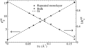
Figure 4: The QE quantities $\epsilon^{QE}_{p}$ and $1/\epsilon^{QE}_{z}$ as functions of the inverse interlayer distance $1/c$, in MoS₂. In each plot, we add the data point corresponding to the bulk.

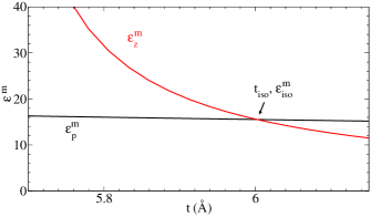
Figure 5: Values of $\epsilon^{m}_{p}$ and $\epsilon^{m}_{z}$ that would be consistent with direct ab initio computation of the supercell’s dielectric constants $\epsilon^{\rm{QE}}_{p}$ and $\epsilon^{\rm{QE}}_{z}$ , as functions of the corresponding thickness of the monolayer. We indicate the point corresponding to an isotropic system.

We now evaluate the dielectric properties of the monolayer using the standard (3D) QE code. We simulate a system made of repeated monolayers separated by a varying distance $c$, with vacuum in between. The clamped-ions dielectric tensor of this system, as computed within QE, is written as

$$\mathcal{E}^{\rm{QE}} =\begin{pmatrix}\epsilon^{\rm{QE}}_{p}&0&0\\ 0&\epsilon^{\rm{QE}}_{p}&0\\ 0&0&\epsilon^{\rm{QE}}_{z}\end{pmatrix}.$$ (9)

In this picture, the dielectric tensor of the bulk simply corresponds to $\mathcal{E}^{\rm{QE}}$ with a fixed interlayer distance $c$ (neglecting the small effects of an alternating stacking). To relate $\mathcal{E}^{\rm{QE}}$ to the dielectric tensor of the monolayer $\mathcal{E}^{m}$, we use effective medium theory and introduce the thickness of the monolayer as a parameter. We then have the following relationsFreysoldt et al. (2008):

$$\begin{split}\epsilon^{\rm{QE}}_{p}&=1+(\epsilon^{m}_{p}-1)t/c\\ \frac{1}{\epsilon^{\rm{QE}}_{z}}&=1-\frac{(\epsilon^{m}_{z}-1)}{\epsilon^{m}_{z}}t/c.\end{split}$$ (10)

Note that in the limit of infinite interlayer distance, this dielectric tensor does not tend toward $\mathcal{E}^{m}$. Instead, it tends towards the dielectric tensor of vacuum.

In Fig. 4, we plot the $\epsilon^{\rm{QE}}_{p}$ and $1/\epsilon^{\rm{QE}}_{z}$ as functions of $1/c$. Fitting this data, we find slopes $s_{1}=87.2$ Å and $s_{2}=5.62$ Å  respectively. We then write $\epsilon^{m}_{p}$ and $\epsilon^{m}_{z}$ as functions of $t$ according to

$$\begin{split}\epsilon^{m}_{p}&=1+\frac{s_{1}}{t}\\ \epsilon^{m}_{z}&=\frac{t}{t-s_{2}}.\end{split}$$ (11)

In principle, every set of values $\{\epsilon^{m}_{p},\epsilon^{m}_{z},t\}$ that satisfies the above equations can fit our DFT results. We can assume that $t>s_{2}$, as we would have $\epsilon^{m}_{z}<0$ otherwise. We can also assume that $t<c_{\rm{bulk}}\approx 6.15$ Å, the distance between two monolayers in the bulk. In the lower panel of Fig. 4, we plot $\epsilon^{m}_{p},\epsilon^{m}_{z}$ as functions of $t$ in this reasonable range of values for the thickness. Fig. 4 should thus be understood as a set of possible values for $\epsilon^{m}_{p},\epsilon^{m}_{z}$ and the corresponding thickness. Note that $t\approx 6$ Å is consistent with the width of the equilibrium electronic density found in DFT. One can see that while $\epsilon^{m}_{p}$ is almost constant in Fig. 4, the variation of $\epsilon^{m}_{z}$ is more pronounced. Similar results are obtained for MoSe₂, MoTe₂, WS₂, and WSe₂. As far as the above ab initio study is concerned, we are thus left with a free parameter to model the dielectric properties of the 2D materials, that is, a choice to make for the set of values $\{\epsilon^{m}_{p},\epsilon^{m}_{z},t\}$. For all TMDs, there is a reasonable value of $t=t_{\rm{iso}}$ leading to an isotropic model with $\epsilon^{m}_{\rm{iso}}=\epsilon^{m}_{p}=\epsilon^{m}_{z}$. As shown in the next section, this isotropic model is a choice that leads to simple yet accurate results for the Fröhlich interaction.

V Effective isotropic model

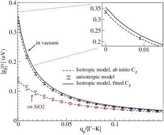
Figure 6: Dashed lines are obtained by using the isotropic model ($\epsilon^{m}_{\rm{iso}}=\epsilon^{m}_{p}=\epsilon^{m}_{z}$, $t=t_{\rm{iso}}$) and $C_{\mathcal{Z}}$ from ab initio Born effective charges. The errors bars show the deviation from the isotropic model obtained by using an anisotropic model with values of $\epsilon^{m}_{p},\epsilon^{m}_{z}$ and $t$ in the range of Fig 5. The plain line corresponds to the isotropic model (for MoS₂ in vacuum) with fitted $C_{\mathcal{Z}}$. This coincides with the direct DFPT calculations of EPC, at least at small momenta (see Figs. 2 and 8). The inset is a zoom on the small momenta limit of the models. It shows that a fitted $C_{\mathcal{Z}}$ is necessary, as an anisotropic model would not be enough to fit the direct DFPT calculations of EPC. The SiO₂ substrate increases the screening of the Fröhlich interaction strongly at small momenta.

We now establish a simple effective model to reproduce the small-momentum limit of our direct DFPT calculations of the coupling to LO phonons. We first discuss the effects of selecting different set of values for $\epsilon^{m}_{p}$, $\epsilon^{m}_{z}$, and $t$. This depends on the dielectric environment, namely on the average dielectric constant $\epsilon_{12}=\frac{\epsilon_{1}+\epsilon_{2}}{2}$. Our DFPT calculations are performed in vacuum, with $\epsilon_{12}=1$. Whatever thickness we choose in Fig. 5, we have $\epsilon^{m}_{p}>>\epsilon_{12}$ and $\epsilon^{m}_{z}>>\epsilon_{12}$. In that case, the anisotropic model is very close to the isotropic one. This is shown numerically in Fig. 6. In dashed lines is the isotropic model, for which we use $\epsilon^{m}_{\rm{iso}}=\epsilon^{m}_{p}=\epsilon^{m}_{z}$ and $t=t_{\rm{iso}}$. The error bars represent the deviation of the full anisotropic model when using other values of $\epsilon^{m}_{p}$, $\epsilon^{m}_{z}$, and $t$ within those represented in Fig. 5.

Table 4: Comparison of relevant quantities involved in the Fröhlich interaction for the monolayer TMDs MoS₂, MoSe₂, MoTe₂, WS₂, and WSe₂. $a_{0}$ si the lattice parameter. We report here the dielectric constants associated to the simplest isotropic model, that is $\epsilon^{m}_{\rm{iso}}=\epsilon^{m}_{p}=\epsilon^{m}_{z}$ and $t=t_{\rm{iso}}$. Note that we use the fact that $r_{\rm{eff}}\approx\epsilon^{m}_{\rm{iso}}t_{\rm{iso}}/2$. For the bare Fröhlich interaction $C_{\mathcal{Z}}$, we report both the fitted value (from fit) used in the plots to reproduce the DFPT data and the value found by computing effective charges and phonons eigenvectors (ab initio).

Monolayer	$a_{0}$(Å)	$t_{\rm{iso}}$ (Å)	$\epsilon^{m}_{\rm{iso}}$	$r_{\rm{eff}}$ (Å)	$C_{\mathcal{Z}}$ (eV) (from fit)	$C_{\mathcal{Z}}$ (eV) (ab initio)	$\omega_{\rm{LO}}$ (cm-1)	$\omega_{\rm{A}_{1}}$ (cm-1)
MoS2	3.18	6.00	15.5	$46.5$	0.355	0.334	373.7	396.9
MoSe2	3.32	5.94	17.9	$53.2$	0.521	0.502	277.5	235.4
MoTe2	3.56	6.65	20.9	$69.5$	0.819	0.819	223.6	162.9
WS2	3.18	5.52	15.2	$42.0$	0.165	0.140	345.9	407.4
WSe2	3.31	5.97	16.3	$48.7$	0.323	0.276	239.4	242.1

For most monolayers, using the bare Fröhlich interaction $C_{\mathcal{Z}}$ calculated via the ab initio effective charges leads to a slight mismatch with respect the direct DFPT calculations of EPC. The effect of anisotropy in vacuum is too small to explain this mismatch, as seen in Fig. 6. To reach better agreement, the parameter $C_{\mathcal{Z}}$ must be adjusted. The fitted values of $C_{\mathcal{Z}}$ for all monolayers are reported in Table 4. Note that ab initio and fitted values stay relatively close, meaning that a simple calculation of the effective charges can still lead to a good approximation of the bare Fröhlich interaction. However, the mismatch is clear enough to point to some possible issues in the computation of the effective charges. This imprecision on the computation of $C_{\mathcal{Z}}$ also implies that we cannot resolve the very small effect of anisotropy.

Overall, an isotropic model with dielectric constant $\epsilon^{m}_{\rm{iso}}=\epsilon^{m}_{p}=\epsilon^{m}_{z}$ and a fitted $C_{\mathcal{Z}}$ (plain lines in Figs 2 and 8 of the Appendix) is the best choice to reproduce our DFPT results. Within the assumption that $\epsilon^{m}_{\rm{iso}}>>\epsilon_{12}$, further simplification and greater clarity can be achieved in the model. Indeed, the parameters of table 1 can be approximated by

$$\epsilon^{0}_{\rm{eff}} \approx\epsilon_{12}=\frac{\epsilon_{1}+\epsilon_{2}}{2}$$ (12)

$$r_{\rm{eff}} \approx\frac{\epsilon^{m}_{\rm{iso}}}{2}t_{\rm{iso}}.$$ (13)

This simple form allows us to gain physical insight on the screening. In the limit $r_{\rm{eff}}|\mathbf{q}_{p}|>>\epsilon_{12}$, that is $|\mathbf{q}_{p}|>>\frac{2\epsilon_{12}}{\epsilon^{m}_{\rm{iso}}t_{\rm{iso}}}$, we have $g^{\rm{2D}}_{\rm{Fr}}(|\mathbf{q}_{p}|)\approx g^{\rm{3D}}_{\rm{Fr}}(|\mathbf{q}_{p}|)$. Indeed, the factor $1/2$ in $r_{\rm{eff}}$ enables to recover the prefactor of the 3D Coulomb interaction ($2\pi e^{2}\to 4\pi e^{2}$), while $At\approx V$, and $\epsilon^{m}_{\rm{iso}}=\epsilon^{m}_{p}\approx\epsilon^{b}_{p}$. In that case, the wavelength of the perturbation associated to the LO phonon is small and the associated field lines stay inside the monolayer. The interaction is then screened by the monolayer. In the $r_{\rm{eff}}|\mathbf{q}_{p}|<<\epsilon_{12}$ limit, that is $|\mathbf{q}_{p}|<<\frac{2\epsilon_{12}}{\epsilon^{m}_{\rm{iso}}t_{\rm{iso}}}$, we have $g^{\rm{2D}}_{\rm{Fr}}(|\mathbf{q}_{p}|)\approx\frac{C_{\mathcal{Z}}}{\epsilon_{12}}$, which corresponds to the interaction being screened solely by the environment. In vacuum, the crossover between those two regimes happens for $|\mathbf{q}_{p}|$ around $\frac{2}{\epsilon^{m}_{\rm{iso}}t_{\rm{iso}}}\approx 0.02$ Å${}^{-1}\approx 0.015|\mathbf{\Gamma-K}|$, that is, very close to the $\mathbf{\Gamma}$ point. This is due to the large dielectric constant of the monolayer compared to the environment.

An important benefit of the model is the possibility to evaluate the effects of the dielectric environmentJena and Konar (2007). In Fig. 6, we present results for the more experimentally relevant case of MoS₂ ion SiO₂, for which $\epsilon_{12}=\frac{1+3.9}{2}=2.45$. The coupling is shown to be strongly decreased overall. The validity of the approximations $\epsilon^{m}_{p}>>\epsilon_{12}$ and $\epsilon^{m}_{z}>>\epsilon_{12}$ is less clear, and the deviation from the isotropic model in Fig. 5 is more discernible. However, for the purpose of estimating the effect of a SiO₂ substrate, and given the simplicity of the above parameters, it is still convenient to use the effective isotropic model.

The relevant parameters, including the thickness $t_{\rm{iso}}$ and isotropic dielectric constant $\epsilon^{m}_{\rm{iso}}$, are reported in Table 4 for all monolayers. In the case of MoS₂, we find that the value of the coupling at $\mathbf{\Gamma}$ in vacuum, i.e. the bare interaction $C_{\mathcal{Z}}$, is three times larger than the one predicted in a previous ab initio studyKaasbjerg et al. (2012). The bare interaction $C_{\mathcal{Z}}$ and effective screening length $r_{\rm{eff}}$ increase with the atomic number of the chalcogen while they decrease with the atomic number of the transition metal.

VI Transport

To provide a more practical sense of the implications of this work, we compute the following inverse relaxation times for an excited electron or hole scattered by LO or A₁ phonons

$$\begin{split}\frac{1}{\tau_{\nu}(\varepsilon_{\mathbf{k}})}=&\frac{2\pi}{\hbar}\sum_{\mathbf{q}_{p}}|g_{\nu}(\mathbf{q}_{p})|^{2}\\ &\times\delta(\varepsilon_{\mathbf{k}+\mathbf{q}_{p}}-\varepsilon_{\mathbf{k}}\mp\hbar\omega_{\mathbf{q}_{p},\nu})\begin{Bmatrix}N_{\nu,\mathbf{q}_{p}}\\ N_{\nu,\mathbf{q}_{p}}+1\end{Bmatrix},\end{split}$$ (14)

where $\nu\equiv$LO or A₁, $N_{\nu,\mathbf{q}_{p}}$ is the Bose-Einstein distribution for phonon occupation at room temperature and $\varepsilon_{\mathbf{k}}$ is the eigenvalue energy of electronic state $|\mathbf{k}\rangle$, measured from the bottom (top) of the conduction (valence) band. The ”$-$” (respectively ”$+$”) sign in the Dirac delta function $\delta$ is associated to $N_{\nu,\mathbf{q}_{p}}$ ($N_{\nu,\mathbf{q}_{p}}+1$) and corresponds to phonon absorption (emission). The two contributions are then summed. In Fig. 7, we plot the inverse relaxation times for each of the three bands (K cond, K val, and $\Gamma$ val) and for each of the MoS₂, MoSe₂, MoTe₂, WS₂, and WSe₂ monolayers. To compute those quantities, we need EPC matrix elements on a fine grid of momenta $\mathbf{q}_{p}$. We use the analytical model when possible and linearly extrapolate the DFPT couplings otherwise. More precisely, in the limit of small momenta, the coupling to LO phonons follows our analytical model of the Fröhlich interaction and does not depend on the angle of momentum $\mathbf{q}_{p}$ or the band. We then use the analytical model $|g^{\rm{2D}}_{\rm{Fr}}(\mathbf{q}_{p})|$. At larger momenta, the coupling depends on the band via the wave functions. We then extrapolate the ab initio coupling $|g_{\rm{LO}}(\mathbf{q}_{p})|$. A few other ab initio calculations were performed for momenta up to $|\mathbf{q}^{\rm{max}}_{p}|\approx 0.3|\mathbf{\Gamma-K}|$. A mild angular dependency is possible for the ab initio matrix elements $|g_{\rm{LO}}(\mathbf{q}_{p})|$ and $|g_{\rm{A_{1}}}(\mathbf{q}_{p})|$. We neglect this angular dependency. The integral of Eq. 14 depends on the coupling and the effective masses of the corresponding band. We use effective masses from Ref. Kormányos et al., 2015, reported in table 5. We probe electronic states with electronic momenta $|\mathbf{k}|<|\mathbf{q}^{\rm{max}}_{p}|/2$. This implies that the range of carrier energies we consider depends on the effective masses. Note that only for MoS₂ is it clear that the valence band at $\Gamma$ should be considered. For the others, this band is lower in energy. For more informations about the band structures of these materials, see Ref. Brumme et al., 2015.

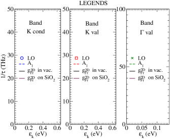
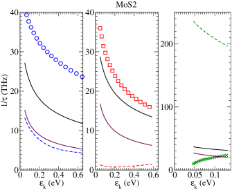
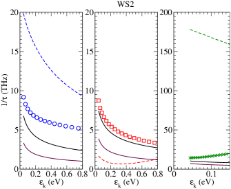
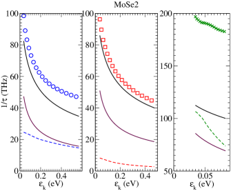
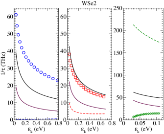
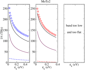
Figure 7: Inverse relaxation times associated to the scattering by LO mode, A₁ mode and the Fröhlich models, for monolayer MoS₂, MoSe₂, MoTe₂, WS₂, and WSe₂. Calculations were performed at room temperature. In the case of the valence band around the $\mathbf{\Gamma}$ point of MoTe2, the effective mass is so large that the norm of the phonon wavevectors $|\mathbf{q}_{p}|$ involved in the scattering processes go beyond the scope of this work. In any case, this band is far below the valence band at $\mathbf{K}$, such that it would not be involved in transport.

Table 5: Effective masses are estimated using the results of Ref. Kormányos et al., 2015.

Monolayer	$m^{*}/m_{0}$ $\mathbf{K}$ cond	$m^{*}/m_{0}$ $\mathbf{K}$ val	$m^{*}/m_{0}$ $\mathbf{\Gamma}$ val
MoS2	0.45	0.57	2.52
MoSe2	0.54	0.65	3.70
MoTe2	0.56	0.72	20.0
WS2	0.31	0.42	2.17
WSe2	0.34	0.45	2.79

Fig. 7 shows that optical phonons are capable of relaxing excited carriers on a timescale inferior to the picosecond at room temperature. The strength of the Fröhlich interaction depends on the material considered, mainly via the variations of Born effective charges. However, this is far from being the only aspect to account for when studying relaxation times. Fig. 7 shows a great disparity of the results depending on the phonon mode, the band, and the material. The analytical model of the Fröhlich interaction is a good estimate of the DFPT calculations only for the valence band at $\mathbf{K}$. The relaxation times depend strongly on the band-specific, large-momentum values of the coupling with LO phonons. This is due to the fact that at the minimum carrier energy ($\varepsilon_{\mathbf{k}}=\hbar\omega_{LO}$), the integral of Eq. 14 already involves relatively large phonon momenta $|\mathbf{q}_{p}|$. The strength of the coupling with A₁ phonons and thus the relative importance of the scattering by LO and A₁ phonons also depends strongly on the bands. Very few comments apply globally. LO phonons seem to dominate optical-phonon scattering around $\mathbf{K}$, for all monolayers except WS₂. A₁ phonons seem to dominate in the valence band around $\mathbf{\Gamma}$ for all monolayers except MoSe₂. Although the analytical model with ab initio parameters is useful for suspended samples in the small momentum limit to interpret the phenomenon, interpolate the coupling or to estimate the effect of the dielectric environment, direct DFPT calculations of EPC for each band is essential. The great disparity in the relaxation times and the number of phenomenon affecting it highlight the need for direct ab initio simulations of electron-phonon interactions in a two-dimensional framework. Furthermore, some additional effects should be included for a quantitative comparison with experiment. This work is a study of the coupling with optical phonons at small-momenta, and should provide useful guidelines to interpret experimental transport data. However, in a full quantitative study of transport properties, one might need to account for spin-orbit coupling, doping effects, the scattering of electrons in the Q band, the scattering between different bands… Those issues can be treated in the framework of QE with 2D Coulomb cutoff.

VII Conclusion

We have implemented the truncation of the Coulomb interaction in the plane-wave and phonon codes of the Quantum ESPRESSO package. This method enables us to simulate the small-momentum limit of the Fröhlich interaction in a 2D framework, for monolayer TMDs MoS₂, MoSe₂, MoTe₂, WS₂, and WSe₂. We show that this limit is three times larger than previously assumed in the case of MoS₂ in vacuum. We develop analytical models for the Fröhlich interaction in 2D materials, along with ab initio methods to evaluate the parameters involved. A simple isotropic model is found to reproduce the small-momentum limit of our DFPT calculations. We provide the parameters of this model for the various TMDs studied. We show that screening is paramount to evaluate the strength of the Fröhlich interaction. In particular the dielectric environment of the 2D material has a strong influence on the small-momentum limit of the interaction. Namely, the interaction is reduced by a factor $\frac{\epsilon_{1}+\epsilon_{2}}{2}$ with respect to vacuum, where $\epsilon_{1}$ and $\epsilon_{2}$ are the dielectric constant of the environment on each side the monolayer. We consider intraband scattering within the valence and conduction bands around $\mathbf{K}$, and within the valence band around $\mathbf{\Gamma}$. Above a certain value of the momentum ($\approx 10\%$ of $|\mathbf{\Gamma-K}|$), the band-dependant form of the electronic wave functions plays a role in the Fröhlich interaction and DFPT calculations are necessary to evaluate deviations from the analytical model. Finally, we evaluate the inverse relaxation times associated to the scattering of photo-excited carriers by LO and A₁ phonons. Those modes are shown to be capable of relaxing carriers on timescales smaller than the picosecond. The efficiency of carrier relaxation by optical phonons in TMDs is found to depend on many parameters. In addition to the strength of the Fröhlich interaction depending on the monolayer, the large momentum, band-specific coupling affects the relaxation times. Depending on the material and the band, the relaxation time associated to the A₁ mode can also be quite large. It is not correct to neglect scattering by either LO or A₁ phonons globally. Overall, the complexity and disparity highlighted in this work points to the necessity of relying on direct ab initio calculations of electron-phonon interactions in a 2D framework.

VIII acknowledgements

The authors would like to thank M. Gibertini for his valuable help in deriving the analytical solution presented in appendix. This project has received funding from the European Union’s Horizon 2020 research and innovation programme under grant agreement No 696656 GrapheneCore1 and by Agence Nationale de la Recherche under the reference no ANR-13-IS10-0003-01. Computer facilities were provided by CINES, IDRIS, and CEA TGCC (grant EDARI n. 2016091202).

Appendix A Analytical model of the 2D Fröhlich interaction

We solve here the model described in the main text, Sec. III.2. The dielectric properties of the system are

$$\mathcal{E}(z)=\begin{cases}\epsilon_{1}\mathcal{I}&\text{if }z<-t/2\\ \mathcal{E}^{m}&\text{if }z<|t/2|\\ \epsilon_{2}\mathcal{I}&\text{if }z>t/2\end{cases}.$$ (15)

The potential $V_{\rm{Fr}}$ must solve the Poisson equation

$$\begin{cases}\nabla\cdot(\mathcal{E}^{m}\nabla V_{\rm{Fr}}(\mathbf{r}_{p},z))=4\pi\nabla\cdot\mathbf{P}(\mathbf{r}_{p},z)&\text{if }|z|<t/2\\ \nabla^{2}V_{\rm{Fr}}(\mathbf{r}_{p},z)=0&\text{if }|z|>t/2\end{cases}.$$ (16)

The associated parallel electric field and orthogonal electric displacement

$$\mathbf{E}^{\parallel}(\mathbf{r}_{p},z) =-\frac{\partial V_{\rm{Fr}}(\mathbf{r}_{p},z)}{\partial\mathbf{r}_{p}},$$ (17)

$$\mathbf{D}^{\perp}(\mathbf{r}_{p},z) =\begin{cases}-\epsilon_{1}\frac{\partial V_{\rm{Fr}}(\mathbf{r}_{p},z)}{\partial z}&\text{if }z<-t/2\\ -\epsilon^{m}_{z}\frac{\partial V_{\rm{Fr}}(\mathbf{r}_{p},z)}{\partial z}&\text{if }|z|<t/2\\ -\epsilon_{2}\frac{\partial V_{\rm{Fr}}(\mathbf{r}_{p},z)}{\partial z}&\text{if }z>t/2\end{cases},$$ (18)

must be continuous.

The general solution to the differential equation of Eq. 16 is the sum of the solution to the homogeneous equation and a particular solution

$$V_{\rm{Fr}}(\mathbf{q}_{p},z)=V_{\rm{h}}(\mathbf{q}_{p},z)+V_{\rm{p}}(\mathbf{q}_{p},z).$$ (19)

The homogeneous equation is

$$\begin{cases}\nabla\cdot(\mathcal{E}^{m}\nabla V_{\rm{h}}(\mathbf{r}_{p},z))=0&\text{if }|z|<t/2\\ \nabla^{2}V_{\rm{h}}(\mathbf{r}_{p},z)=0&\text{if }|z|>t/2\end{cases},$$ (20)

and the particular solution solves Eq. 16. To find a particular solution, we first solve Eq. 16 inside the anisotropic material:

$$\nabla\cdot(\mathcal{E}^{m}\nabla V_{\rm{p}}(\mathbf{r})) =4\pi e^{2}\frac{i|\mathbf{q}_{p}|}{A}\times$$ (21)

$$\ \ \sum_{a}\frac{\mathbf{e}_{\mathbf{q}_{p}}\cdot\mathcal{Z}_{a}^{m}\cdot\mathbf{e}^{a}_{\mathbf{q}_{p}\rm{LO}}}{\sqrt{2M_{a}\omega_{\mathbf{q}_{p}\rm{LO}}}}f(z)e^{i\mathbf{q}_{p}\cdot\mathbf{r}_{p}}$$ (22)

$$V_{\rm{p}}(\mathbf{q}_{p},q_{z}) =\frac{-2iC_{\mathcal{Z}}|\mathbf{q}_{p}|}{\epsilon^{m}_{p}|\mathbf{q}_{p}|^{2}+\epsilon^{m}_{z}q_{z}^{2}}f(q_{z})$$ (23)

$$V_{\rm{p}}(\mathbf{q}_{p},z) =\frac{-iC_{\mathcal{Z}}}{\sqrt{\epsilon^{m}_{p}\epsilon^{m}_{z}}}\int_{-\infty}^{+\infty}e^{-\tilde{\mathbf{q}}_{p}|z^{\prime}-z|}f(z^{\prime})dz^{\prime}$$ (24)

with $\tilde{\mathbf{q}}_{p}=\sqrt{\frac{\epsilon^{m}_{p}}{\epsilon^{m}_{z}}}\mathbf{q}$, and $C_{\mathcal{Z}}$ is defined in table 1. Using $f(z^{\prime})=\frac{\theta(t/2-|z^{\prime}|)}{t}$ we get for $z\in[-t/2;t/2]$

$$V_{\rm{p}}(\mathbf{q}_{p},z) =\frac{-iC_{\mathcal{Z}}}{\sqrt{\epsilon^{m}_{p}\epsilon^{m}_{z}}}\frac{2}{|\tilde{\mathbf{q}}_{p}|t}\left(1-e^{-|\tilde{\mathbf{q}}_{p}|t/2}{\rm{cosh}}(|\tilde{\mathbf{q}}_{p}|z)\right),$$ (25)

where $\rm{cosh}$ is the hyperbolic cosine function. We need to extend this particular solution outside the material. We do not require the particular solution to carry any physical meaning outside the material. It only needs to fulfil

$$\nabla^{2}V_{\rm{p}}(\mathbf{r}_{p},z) =0\ \ \ \text{if }|z|>t/2.$$ (26)

We simply choose the solution of the above equation such that the corresponding out-of-plane electric field is continuous at the interfaces. This solution exist, and since we will only need its values at the interfaces, it is not necessary to specify it further.

Let us proceed to the homogeneous solution. Knowing that $V_{h}(\mathbf{r})=V_{h}(\mathbf{q}_{p},z)e^{i\mathbf{q}_{p}\cdot\mathbf{r}_{p}}$ , the homogeneous equation Eq. 20 reduces to

$$\begin{cases}\frac{\partial^{2}V_{h}(\mathbf{q}_{p},z)}{\partial z^{2}}&=\frac{\epsilon^{m}_{p}}{\epsilon^{m}_{z}}|\mathbf{q}_{p}|^{2}V_{h}(\mathbf{q}_{p},z)\text{ if }|z|<t/2\\ \frac{\partial^{2}V_{h}(\mathbf{q}_{p},z)}{\partial z^{2}}&=|\mathbf{q}_{p}|^{2}V_{h}(\mathbf{q}_{p},z)\text{ if }|z|>t/2\end{cases}.$$ (27)

Adding the condition that the potential must vanish for $|z|\to\infty$, the solution to the homogeneous equation Eq. 20 has the form:

$$V_{h}(\mathbf{q}_{p},z)=\begin{cases}c_{3}e^{-|\mathbf{q}_{p}|z}&\text{if }z>t/2\\ c_{1}e^{|\tilde{\mathbf{q}}_{p}|z}+c_{2}e^{-|\tilde{\mathbf{q}}_{p}|z}&\text{if }|z|<t/2\\ c_{4}e^{|\mathbf{q}_{p}|z}&\text{if }z<-t/2\end{cases}$$ (28)

with $\tilde{\mathbf{q}}_{p}=\sqrt{\frac{\epsilon^{m}_{p}}{\epsilon^{m}_{z}}}\mathbf{q}$. Note that the homogeneous solution has the form of a potential generated by 2 surface charges at the interfaces of the monolayer. The continuity of the potential gives

$$c_{3}e^{-|\mathbf{q}_{p}|t/2} =c_{1}e^{|\tilde{\mathbf{q}}_{p}|t/2}+c_{2}e^{-|\tilde{\mathbf{q}}_{p}|t/2},$$ (29)

$$c_{4}e^{-|\mathbf{q}_{p}|t/2} =c_{1}e^{-|\tilde{\mathbf{q}}_{p}|t/2}+c_{2}e^{|\tilde{\mathbf{q}}_{p}|t/2}.$$ (30)

The continuity of the parallel electric field is fulfilled by construction. We use the continuity of the out-of-plane electric displacement Eq. 18 to obtain

$$\begin{cases}\frac{C_{\mathcal{Z}}}{\sqrt{\epsilon^{m}_{p}\epsilon^{m}_{z}}}(\epsilon^{m}_{z}-\epsilon_{1})\frac{1-e^{-|\tilde{\mathbf{q}}_{p}|t}}{|\mathbf{q}_{p}|t}&=(\epsilon_{1}+\sqrt{\epsilon^{m}_{p}\epsilon^{m}_{z}})c_{1}e^{|\tilde{\mathbf{q}}_{p}|t/2}+(\epsilon_{1}-\sqrt{\epsilon^{m}_{p}\epsilon^{m}_{z}})c_{2}e^{-|\tilde{\mathbf{q}}_{p}|t/2}\\ \frac{C_{\mathcal{Z}}}{\sqrt{\epsilon^{m}_{p}\epsilon^{m}_{z}}}(\epsilon^{m}_{z}-\epsilon_{2})\frac{1-e^{-|\tilde{\mathbf{q}}_{p}|t}}{|\mathbf{q}_{p}|t}&=(\epsilon_{2}-\sqrt{\epsilon^{m}_{p}\epsilon^{m}_{z}})c_{1}e^{-|\tilde{\mathbf{q}}_{p}|t/2}+(\epsilon_{2}+\sqrt{\epsilon^{m}_{p}\epsilon^{m}_{z}})c_{2}e^{|\tilde{\mathbf{q}}_{p}|t/2}\end{cases}.$$ (31)

By defining the following dielectric mismatches

$$\alpha_{1}=\frac{\epsilon^{m}_{z}-\epsilon_{1}}{\sqrt{\epsilon^{m}_{p}\epsilon^{m}_{z}}+\epsilon_{1}} \bar{\alpha}_{2}=\frac{\sqrt{\epsilon^{m}_{p}\epsilon^{m}_{z}}-\epsilon_{2}}{\sqrt{\epsilon^{m}_{p}\epsilon^{m}_{z}}+\epsilon_{2}}$$

$$\alpha_{2}=\frac{\epsilon^{m}_{z}-\epsilon_{2}}{\sqrt{\epsilon^{m}_{p}\epsilon^{m}_{z}}+\epsilon_{2}} \bar{\alpha}_{1}=\frac{\sqrt{\epsilon^{m}_{p}\epsilon^{m}_{z}}-\epsilon_{1}}{\sqrt{\epsilon^{m}_{p}\epsilon^{m}_{z}}+\epsilon_{1}},$$ (32)

we finally have

$$c_{1} =\frac{C_{\mathcal{Z}}}{\sqrt{\epsilon^{m}_{p}\epsilon^{m}_{z}}}\frac{1-e^{-|\tilde{\mathbf{q}}_{p}|t}}{|\mathbf{q}_{p}|t}\frac{\alpha_{1}+\bar{\alpha}_{1}\alpha_{2}e^{-|\tilde{\mathbf{q}}_{p}|t}}{1-\bar{\alpha}_{1}\bar{\alpha}_{2}e^{-2|\tilde{\mathbf{q}}_{p}|t}}e^{-|\tilde{\mathbf{q}}_{p}|t/2}$$ (33)

$$c_{2} =\frac{C_{\mathcal{Z}}}{\sqrt{\epsilon^{m}_{p}\epsilon^{m}_{z}}}\frac{1-e^{-|\tilde{\mathbf{q}}_{p}|t}}{|\mathbf{q}_{p}|t}\frac{\alpha_{2}+\bar{\alpha}_{2}\alpha_{1}e^{-|\tilde{\mathbf{q}}_{p}|t}}{1-\bar{\alpha}_{1}\bar{\alpha}_{2}e^{-2|\tilde{\mathbf{q}}_{p}|t}}e^{-|\tilde{\mathbf{q}}_{p}|t/2}.$$ (34)

The Fröhlich interaction is thus

$$g^{\rm{2D}}_{\rm{Fr}}(\mathbf{q}_{p})=\frac{1}{t}\int_{-t/2}^{t/2}\left(V_{\rm{p}}(\mathbf{q}_{p},z)+V_{h}(\mathbf{q}_{p},z)\right)dz$$ (35)

$$g^{\rm{2D}}_{\rm{Fr}}(\mathbf{q}_{p})=\frac{C_{\mathcal{Z}}}{\sqrt{\epsilon^{m}_{p}\epsilon^{m}_{z}}}\left[\frac{2}{|\tilde{\mathbf{q}}_{p}|t}\left(1+\frac{e^{-|\tilde{\mathbf{q}}_{p}|t}-1}{|\tilde{\mathbf{q}}_{p}|t}\right)\right.$$ (36)

$$\left.+\frac{(1-e^{-|\tilde{\mathbf{q}}_{p}|t})^{2}}{|\mathbf{q}_{p}|t|\tilde{\mathbf{q}}_{p}|t}\frac{\alpha_{1}+\alpha_{2}+(\bar{\alpha}_{1}\alpha_{2}+\bar{\alpha}_{2}\alpha_{1})e^{-|\tilde{\mathbf{q}}_{p}|t}}{1-\bar{\alpha}_{1}\bar{\alpha}_{2}e^{-2|\tilde{\mathbf{q}}_{p}|t}}\right].$$

The isotropic solution is ($\epsilon^{m}_{p}=\epsilon^{m}_{z}=\epsilon^{m}_{\rm{iso}}$):

$$g^{\rm{2D}}_{\rm{Fr}}(\mathbf{q}_{p}) =\frac{C_{\mathcal{Z}}}{\epsilon^{m}_{\rm{iso}}}\left[\frac{2}{|\mathbf{q}_{p}|t}\left(1+\frac{e^{-|\mathbf{q}_{p}|t}-1}{|\mathbf{q}_{p}|t}\right)\right.$$ (37)

$$\left.+\frac{(1-e^{-|\mathbf{q}_{p}|t})^{2}}{(|\mathbf{q}_{p}|t)^{2}}\frac{\alpha_{1}+\alpha_{2}+2\alpha_{1}\alpha_{2}e^{-|\mathbf{q}_{p}|t}}{1-\alpha_{1}\alpha_{2}e^{-2|\mathbf{q}_{p}|t}}\right]$$

Appendix B Coupling with optical phonons in TMDs

In Fig. 8 we plot the small-momentum coupling to the A₁ and LO modes in monolayer TMDs MoS₂, MoSe₂, MoTe₂, WS₂, and WSe₂. Note that that WSe₂ is similar to MoS₂. WS₂ shows significantly smaller Frohlich interaction. MoSe₂ and MoTe₂ are similar to each other, with large Fröhlich interaction and some different trends in the A₁ mode. Note also that the analytical model coincides relatively well with the DFPT results for the valence band at $\mathbf{K}$ in every material.

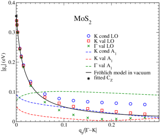
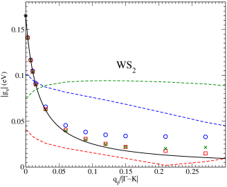
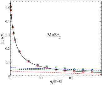
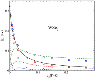
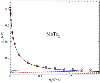
Figure 8: EPC matrix elements involving LO and A₁ phonon modes in monolayer MoS₂, MoSe₂, MoTe₂, WS₂ and WSe₂. We consider intraband scattering of electrons or holes in the conduction band near $\mathbf{K}$ (”K cond”)  and in the valence band near $\mathbf{K}$ and $\mathbf{\Gamma}$ (”K val” and ”$\mathbf{\Gamma}$ val”, respectively). Momenta $\mathbf{q}_{p}$ are in the $\mathbf{\Gamma}\to\mathbf{M}$ direction. The analytical model of the Frohlich interaction in its simplest isotropic form and using the parameters indicated in Table 4 is shown in black plain lines. Dashed lines and symbols are DFPT calculations.

References

- Radisavljevic et al. (2011) Branimir Radisavljevic, Aleksandra Radenovic, Jacopo Brivio, V. Giacometti, and Andras Kis, “Single-layer MoS2 transistors,” Nature nanotechnology 6, 147–50 (2011), arXiv:0402594v3 [arXiv:cond-mat] .
- Wang et al. (2012) Qing Hua Wang, Kourosh Kalantar-Zadeh, Andras Kis, Jonathan N Coleman, and Michael S Strano, “Electronics and optoelectronics of two-dimensional transition metal dichalcogenides,” Nature Nanotechnology 7, 699–712 (2012).
- Jariwala et al. (2014) Deep Jariwala, Vinod K. Sangwan, Lincoln J. Lauhon, Tobin J. Marks, and Mark C. Hersam, “Emerging device applications for semiconducting two-dimensional transition metal dichalcogenides,” ACS Nano 8, 1102–1120 (2014), arXiv:1402.0047 .
- Ganatra and Zhang (2014) Rudren Ganatra and Qing Zhang, “Few-layer MoS2: A promising layered semiconductor,” ACS Nano 8, 4074–4099 (2014).
- Fiori et al. (2014) Gianluca Fiori, Francesco Bonaccorso, Giuseppe Iannaccone, Tomás Palacios, Daniel Neumaier, Alan Seabaugh, Sanjay K. Banerjee, and Luigi Colombo, “Electronics based on two-dimensional materials,” Nature Nanotechnology 9, 768–779 (2014).
- Moody et al. (2015) Galan Moody, Chandriker Kavir Dass, Kai Hao, Chang-Hsiao Chen, Lain-Jong Li, Akshay Singh, Kha Tran, Genevieve Clark, Xiaodong Xu, Gunnar Berghäuser, Ermin Malic, Andreas Knorr, and Xiaoqin Li, “Intrinsic homogeneous linewidth and broadening mechanisms of excitons in monolayer transition metal dichalcogenides,” Nature Communications 6, 8315 (2015).
- Wang et al. (2015) Haining Wang, Changjian Zhang, and Farhan Rana, “Ultrafast dynamics of defect-assisted electron-hole recombination in monolayer MoS2,” Nano Letters 15, 339–345 (2015), arXiv:1409.4518 .
- Shi et al. (2013) Hongyan Shi, Rusen Yan, Simone Bertolazzi, Jacopo Brivio, Bo Gao, Andras Kis, Debdeep Jena, Huili Grace Xing, and Libai Huang, “Exciton dynamics in suspended monolayer and few-layer MoS2 2D crystals,” ACS Nano 7, 1072–1080 (2013).
- Baroni et al. (2001) Stefano Baroni, Stefano De Gironcoli, Andrea Dal Corso, and Paolo Giannozzi, “Phonons and related crystal properties from density-functional perturbation theory,” Reviews of Modern Physics 73, 515–562 (2001), arXiv:0012092v1 [arXiv:cond-mat] .
- Vogl (1976) Peter Vogl, “Microscopic theory of electron-phonon interaction in insulators or semiconductors,” Physical Review B 13, 694–704 (1976).
- Sarma and Mason (1985) Sankar Das Sarma and Bruce A. Mason, “Optical phonon interaction effects in layered semiconductor structures,” Annals of Physics 163, 78–119 (1985).
- Mori and Ando (1989) Nobuya Mori and Tsuneya Ando, “Electronoptical-phonon interaction in single and double heterostructures,” Physical Review B 40, 6175–6188 (1989).
- Sjakste et al. (2015) Jelena Sjakste, Nathalie Vast, Matteo Calandra, and Francesco Mauri, “Wannier interpolation of the electron-phonon matrix elements in polar semiconductors: Polar-optical coupling in GaAs,” Physical Review B - Condensed Matter and Materials Physics 92, 054307 (2015), arXiv:1508.06172 .
- Sohier et al. (2015) Thibault Sohier, Matteo Calandra, and Francesco Mauri, “Density-functional calculation of static screening in two-dimensional materials: The long-wavelength dielectric function of graphene,” Physical Review B - Condensed Matter and Materials Physics 91, 165428 (2015), arXiv:1503.02530v1 .
- Keldysh (1979) Leonid V. Keldysh, “Coulomb interaction in thin semiconductor and semimetal films,” JETP Letters 29, 658–661 (1979).
- Cudazzo et al. (2011) Pierluigi Cudazzo, Ilya V. Tokatly, and Angel Rubio, “Dielectric screening in two-dimensional insulators: Implications for excitonic and impurity states in graphane,” Physical Review B - Condensed Matter and Materials Physics 84, 085406 (2011), arXiv:1104.3346 .
- Wehling et al. (2011) Tim O. Wehling, Ersoy Sasioglu, Christoph Friedrich, Alexander I. Lichtenstein, Mikhail I. Katsnelson, and Stefan Blügel, “Strength of effective coulomb interactions in graphene and graphite,” Physical Review Letters 106, 236805 (2011), arXiv:1101.4007 .
- Berkelbach et al. (2013) Timothy C. Berkelbach, Mark S. Hybertsen, and David R. Reichman, “Theory of neutral and charged excitons in monolayer transition metal dichalcogenides,” Physical Review B - Condensed Matter and Materials Physics 88, 045318 (2013), arXiv:1305.4972 .
- Steinhoff et al. (2014) Alexander Steinhoff, M. Rösner, Frank Jahnke, Tim O. Wehling, and Christopher Gies, “Influence of excited carriers on the optical and electronic properties of MoS2,” Nano Letters 14, 3743–3748 (2014).
- Kaasbjerg et al. (2012) Kristen Kaasbjerg, Kristian S. Thygesen, and Karsten W. Jacobsen, “Phonon-limited mobility in n-type single-layer MoS 2 from first principles,” Physical Review B - Condensed Matter and Materials Physics 85, 115317 (2012), arXiv:1201.5284 .
- Li et al. (2013) Xiaodong Li, Jeffrey T. Mullen, Zhenghe Jin, Kostyantyn M. Borysenko, M. Buongiorno Nardelli, and Ki Wook Kim, “Intrinsic electrical transport properties of monolayer silicene and MoS2 from first principles,” Physical Review B - Condensed Matter and Materials Physics 87, 115418 (2013), arXiv:arXiv:1301.7709v1 .
- Jin et al. (2014) Zhenghe Jin, Xiaodong Li, Jeffrey T. Mullen, and Ki Wook Kim, “Intrinsic transport properties of electrons and holes in monolayer transition-metal dichalcogenides,” Physical Review B - Condensed Matter and Materials Physics 90, 045422 (2014), arXiv:1406.4569 .
- Danovich et al. (2015) Mark Danovich, Igor Aleiner, Neil D. Drummond, and Vladimir Fal’ko, “Fast relaxation of photo-excited carriers in 2D transition metal dichalcogenides,” arXiv , 13–16 (2015), arXiv:1510.06288 .
- Sohier (2015) Thibault Sohier, Electrons and phonons in graphene : electron-phonon coupling, screening and transport in the field effect setup, Phd thesis, Universite Pierre et Marie Curie, Paris VI (2015).
- Giannozzi et al. (2009) Paolo Giannozzi, Stefano Baroni, Nicola Bonini, Matteo Calandra, Roberto Car, Carlo Cavazzoni, Davide Ceresoli, Guido L Chiarotti, Matteo Cococcioni, Ismaila Dabo, Andrea Dal Corso, Stefano de Gironcoli, Stefano Fabris, Guido Fratesi, Ralph Gebauer, Uwe Gerstmann, Christos Gougoussis, Anton Kokalj, Michele Lazzeri, Layla Martin-Samos, Nicola Marzari, Francesco Mauri, Riccardo Mazzarello, Stefano Paolini, Alfredo Pasquarello, Lorenzo Paulatto, Carlo Sbraccia, Sandro Scandolo, Gabriele Sclauzero, Ari P Seitsonen, Alexander Smogunov, Paolo Umari, and Renata M Wentzcovitch, “QUANTUM ESPRESSO: a modular and open-source software project for quantum simulations of materials.” Journal of Physics: Condensed Matter 21, 395502 (2009), arXiv:0906.2569 .
- Note (1) I. E. Castelli et al. in preparation (2016), see http://www.materialscloud.org/sssp.
- Podberezskaya et al. (2001) Nina V. Podberezskaya, Svetlana A. Magarill, Natal’ya V. Pervukhina, and Stanislav V. Borisov, “Crystal chemistry of dichalcogenides MX2,” Journal of Structural Chemistry 42, 654–681 (2001).
- Brumme et al. (2015) Thomas Brumme, Matteo Calandra, and Francesco Mauri, “First-principles theory of field-effect doping in transition-metal dichalcogenides: Structural properties, electronic structure, Hall coefficient, and electrical conductivity,” Physical Review B - Condensed Matter and Materials Physics 91, 155436 (2015), arXiv:1501.07223 .
- Molina-Sánchez and Wirtz (2011) Alejandro Molina-Sánchez and Ludger Wirtz, “Phonons in single-layer and few-layer MoS2 and WS2,” Physical Review B - Condensed Matter and Materials Physics 84, 155413 (2011), arXiv:1109.5499 .
- Tóbik and Dal Corso (2004) Jaroslav Tóbik and Andrea Dal Corso, “Electric fields with ultrasoft pseudo-potentials: Applications to benzene and anthracene,” Journal of Chemical Physics 120, 9934–9941 (2004), arXiv:0403291 [cond-mat] .
- Yu et al. (2008) Eric K. Yu, Derek A. Stewart, and Sandip Tiwari, “Ab initio study of polarizability and induced charge densities in multilayer graphene films,” Physical Review B - Condensed Matter and Materials Physics 77, 195406 (2008).
- Freysoldt et al. (2008) Christoph Freysoldt, Philipp Eggert, Patrick Rinke, Arno Schindlmayr, and Matthias Scheffler, “Screening in two dimensions: GW calculations for surfaces and thin films using the repeated-slab approach,” Physical Review B - Condensed Matter and Materials Physics 77, 235428 (2008), arXiv:0801.1714 .
- Jena and Konar (2007) Debdeep Jena and Aniruddha Konar, “Enhancement of carrier mobility in semiconductor nanostructures by dielectric engineering,” Physical Review Letters 98, 136805 (2007), arXiv:0707.2244 .
- Kormányos et al. (2015) Andor Kormányos, Guido Burkard, Martin Gmitra, Jaroslav Fabian, Viktor Zólyomi, Neil D Drummond, and Vladimir Fal’ko, “K · P Theory for Two-Dimensional Transition Metal Dichalcogenide Semiconductors,” 2D Materials 2, 022001 (2015), arXiv:1410.6666 .