The Shape of Dark Matter Haloes
V. Analysis of observations of edge-on galaxies

Abstract

In the previous papers in this series, we have measured the stellar and HI content in a sample of edge-on galaxies. In the present paper, we perform a simultaneous rotation curve and vertical force field gradient decomposition for five of these edge-on galaxies. The rotation curve decomposition provides a measure of the radial dark matter potential, while the vertical force field gradient provide a measure of the vertical dark matter potential. We fit dark matter halo models to these potentials. Using our HI self-absorption results, we find that a typical dark matter halo has a less dense core ($0.094\pm 0.230$ M_⊙/pc³) compared to an optically thin HI model ($0.150\pm 0.124$ M_⊙/pc³). The HI self-absorption dark matter halo has a longer scale length $R_{c}$ of $1.42\pm 3.48$ kpc, versus $1.10\pm 1.81$ kpc for the optically thin HI model. The median halo shape is spherical, at $q=1.0\pm 0.6$ (self-absorbing HI ), while it is prolate at $q=1.5\pm 0.6$ for the optically thin. Our best results were obtained for ESO 274-G001 and UGC 7321, for which we were able to measure the velocity dispersion in Paper III. These two galaxies have drastically different halo shapes, with one oblate and one strongly prolate. Overall, we find that the many assumptions required make this type of analysis susceptible to errors.

1 Introduction

Modern day cosmological dark matter simulations predict that dark matter has a significant impact on the formation and evolution of galaxies. The dark matter clumps into haloes, which serve as gravitational sinks for baryonic matter to fall in to. Once inside, these baryons form the galaxies and other visible structures in the universe. The size and shape of these haloes is influenced by the type of dark matter particle and its merger history. As such, getting a grip on the shape of the halo offers a potential constraint on the dark matter model (Davis et al., 1985).

The shape of dark matter haloes can be classified by the shape parameter $q$, using the ratios between the vertical axis $c$ and radial axis $a$, such that $q=c/a$. This divides the potential halo shapes up into three classes: prolate ($q>1$), oblate ($q<1$) and spherical ($q\sim 1$). This is, of course, only a simplified version of reality, where we can also expect triaxial shapes and changes of shape with radius and history (Vera-Ciro et al., 2014). However, for haloes with masses $\lower 2.15277pt\hbox{$\;\buildrel>\over{\sim}\;$}10^{12.3}h^{-1}M_{\odot}$ the haloes can be adequately described by a single vertical-to-radial axis ratio (Schneider et al., 2012).

Direct observations of the shape of haloes is tricky, as there are only few tracers that offer a clear view on the vertical gravitational potential of the halo. The flat rotation curves of galaxies, while an excellent tracer of the radial potential of the halo, provides no information in the vertical direction. Luckily, some tracers do exist. The stellar streams of stripped, in-falling galaxies can be used to measure the potential the stream is traversing. Helmi (2004) analysed the stream of Sagittarius, as found in the 2MASS survey, around the Galaxy and found that the data best fits a model with a prolate shape, with an axis ratio of 5/3. In a similar fashion, only further out, do the satellites of the Galaxy offer such a tracer. Globular cluster NGC 5466 was modelled by Lux et al. (2012) and found to favor an oblate or triaxial halo, while excluding spherical and prolate haloes with a high confidence. The stellar stream has been reanalysed by Vera-Ciro & Helmi (2013), who report an oblate halo with $q=0.9$ for $r\leq 10$ kpc.

Gravitational lensing offers another measure of the vertical gravitational potential. Strong lensing uses the Einstein lens of background sources around a single galaxy or cluster. By modelling the lens, it is possible to create a detailed mass map of the system. By combining this with gas and stellar kinematics, it is possible to calculate the dark matter mass distribution (Treu, 2010). For example, Barnabè et al. (2012) applied this method to lensed galaxy SDSS  J2141, to find a slightly oblate halo ($q=0.91^{+0.15}_{-0.13}$).

Weak lensing lacks the clear gravitation lens seen in strong lensing. As such, it is unable to measure the halo of a single galaxy. Instead, it provides an average halo shape from a statistically large sample of sources, by modelling the alignment of background galaxies to a large series of foreground galaxies. This allows the sources to probe the outer edges of haloes. A recent analysis by van Uitert et al. (2012) finds, on a sample of $2.2\times 10^{7}$ galaxies, that the halo ellipticity distribution favors oblate, with $q=0.62^{+0.25}_{-0.26}$.

Polar ring galaxies are also of interest in the study of the dark matter halo shape, as the orbits of the stars in the polar rings are very sensitive to the gravitational potential. The method was pioneered by Schweizer et al. (1983) who noted that the polar ring in galaxy A0136-0801 indicated a massive halo that was more spherical than flat. Whitmore et al. (1987) studied this galaxy in more detail and found $q=0.98\pm 0.20$ for this galaxy. These authors also studied galaxies NGC 4650A and ESO 415-G26, for which they report $q=0.86\pm 0.21$ and $q=1.05\pm 0.17$. Galaxy NGC 4650A has also been studied by Sackett et al. (1994), who reported a flattened halo with $q$ between 0.3 and 0.4.

Another way to place constraints on the halo shape is by carefully modelling local edge-on galaxies. The thickness of the HI layer in spiral galaxies corresponds directly on the local hydrostatic equilibrium. The HI layer flares out at large radii, as there is less matter gravitationally binding it to the central plane. Because of this, flaring provides a sensitive tracer of the vertical potential as a function of radius in the disc. By combining this with the horizontal potential as gained from the rotation curve, and estimates for the gas and stellar mass distributions, one can fit the potential well created by the dark matter halo. This method was first applied to the Galaxy by Celnik et al. (1979) and by van der Kruit (1981) on edge-on galaxy NGC 891. In the latter it was found that the halo was spherical rather than flattened as the stellar disc. NGC 4244 was analysed by Olling (1995), who found a highly flattened halo of $q=0.2^{+0.3}_{-0.1}$. O’Brien et al. (2010) also set out to measure the velocity dispersion as function of radius. Using that approach to measure the halo shape of UGC 7321, they found a spherical halo ($q=1.0\pm 0.1$).

This paper is the fifth in a series. We will refer to earlier papers of the series simply as Papers I through IV. In this paper V, we will perform a similar analysis, using the measured parameters for the HI disc (Paper III) and stellar disc (Paper IV). The series is based on a large part of the PhD thesis of the first author (Peters, 2014). The paper has the following outline. In Section 2, we will provide a detailed description of hydrostatic models we use and detail the fitting strategy. Section 3 presents and discusses the results. We summarise the results in Section 4

2 Modelling Strategy

2.1 Overall Strategy & Sample

Celnik et al. (1979) proposed a new strategy in which the flaring of the HI layers is used as a tracer of the vertical gravitational potential in the Galaxy. This method was extended to edge-on galaxy NGC 891 by van der Kruit (1981). In combination with a traditional rotation curve decomposition, this offers a view on both the radial and vertical directions of the gravitational potential. The dark matter halo model can be fit to this. Further previous work on this subject, using the flaring of gas layers, includes that by Olling (1995, 1996), Olling & Merrifield (2000), Combes & Becquaert (1997), Narayan et al. (2005), Kalberla (2003), Kalberla et al. (2007) and Banerjee & Jog (2008a), and others.

We will use this same strategy to model the dark matter halo shape for the sample of eight galaxies defined in Paper I and extensively studied in further papers in this series. In Paper III, we have measured the structure and kinematics of the HI in these galaxies, using modelling procedures that allow for the correction of self-absorption in the HI for assumed spin temperatures. The stellar discs were modelled in Paper IV. Based on the quality of the results from Papers III and IV, we have decided to model five out of the original eight galaxies in our sample. These are IC 5249, ESO 115-G021, ESO 138-G014, ESO 274-G001 and UGC 7321. All five galaxies are late-type Sd, with self-absorption corrected HI masses between $4.1\!\pm\!0.1\!\times\!10^{8}$ and $7.8\!\pm\!0.8\!\times 10^{9}$ M_⊙ (Table 1 in Paper III). The distances vary greatly between these galaxies. ESO 274-G001 is only 3.0 Mpc away, while the distance to IC 5249 is estimated at 32.1 Mpc.

In Paper III, we successfully measured the velocity dispersion of the HI as function of radius in ESO 274-G001 and UGC 7321. In ESO 115-G021, the velocity dispersion appeared to increase with radius from about 7 km s^-1in the inner parts to 12-14 km s^-1at the outer measured point. As we are skeptical of this result, we will adopt a constant velocity dispersion of 10 km/s for this galaxy. We also adopt this constant velocity dispersion for IC 5249 and ESO 138-G014. For UGC7321 the velocity dispersion drops from 10 km s^-1in the central parts to 8 km s^-1at 8 kpc, then remains constant at this level out to 10 kpc, after wich it increases to 12 km s^-1at 14 kpc. We have sufficient confidence in it to adopt it in our analysis.

Galaxy UGC 7321 has a total B-band magnitude of 13.75 and V-band magnitude of 13.19 (Taylor et al., 2005), giving a B-V band difference of 0.56. To estimate the stellar mass to light ($M_{*}/L_{R}$) ratio, we use the model interpolation engine, which is based on the Worthey (1994) and Bertelli et al. (1994) stellar population models. Using a single burst, Salpeter (slope -2.35) IMF we find a good fit using a single population of 950 Myr and [Fe/H]=0.0, with B-V=0.554. This would place $M_{*}/L_{R}$ in the Rc-band at 0.55. We have repeated this exercise for our other galaxies, each time finding $M_{*}/L_{R}\approx 0.5$. We therefore adopt a mass to light $M_{*}/L_{R}=0.5$ as a lower boundary to the stellar disc mass, and use the reported R-band total luminosities reported in Table 3 of Paper IV. As an upper boundary, we adopt $M_{*}/L_{R}<3$. At solar metallicity, this would imply a single stellar population of approximately 8 Myr. At multiplicities lower than solar, this would increase to an even large age.

2.2 Decomposition Strategy

We start with the assumption that there are three components, stars, gas+dust and dark matter. Each of these components add to the gravitational potential, so ideally one would need to write down and solve the combined Poisson-Boltzmann equation. This is internally consistent, but requires simplifying assumptions such as on the properties of the stellar velocity tensor (e.g. that it is Gaussian and isothermal or a superposition of such components) and its variation in space. This approach, which indeed is self-consistent, has been used by the earlier workers referred to above, starting with Olling (1996).

Our stategy is the following. We infer the radial force near the plane of the galaxy from the HI rotation curve, assuming that due to the relative low velocity dispersion of order 10 km s^-1the asymetric drift term in the Jeans equation can be ignored. Next we model the light distribution and assuming a constant mass-to-light ratio estimate the contribution of the disk up the a free parameter $M/L$. We do the same from the inferred mass distribution of gas, adding the usual contribution (25% of the total) for helium. We assume also that the molecular gas content in these late-type dwarfs is small. This gives us (except for the parameter $M/L$) the gradient in the radial force due to the halo. We next estimate the vertical force from the thickness and velocity dispersion of the HI , using the vertical Jeans equation. Since we evaluate the forces at $z=100$ pc, this should be an excellent approximation, even though the equations used are not internally self-consistent as in the approach in the first paragraph. This strategy has previously been used by O’Brien et al. (2010).

2.2.1 Radial Tracer

The radial force gradient is calculated using a classic rotation curve decomposition performed at the mid-plane of the galaxy (van Albada et al., 1985):

$$v_{\textrm{total}}^{2}(R)=v_{\textrm{gas}}^{2}(R)+v_{\textrm{stellar}}^{2}(R)+v_{\textrm{halo}}^{2}(R)\,\,.$$ (1)

The total rotation $v_{\textrm{total}}(R)$ is the observed rotation curve of the HI gas, as we measured previously in Paper III. The theoretical rotation curves of the gas $v_{\textrm{gas}}(R)$ and stars $v_{\textrm{stellar}}(R)$ represent the contributions due to the stellar and gaseous mass components. We calculate the theoretical rotation curve of the stellar and gaseous components, using equation (A.17) of Casertano (1983)

$$v^{2}(R)=-8GR\int_{0}^{\infty}r\int_{0}^{\infty}\frac{\partial\rho(r,z)}{\partial r}\frac{K(p)-E(p)}{(Rrp)^{1/2}}\,dz\,dr\,\,,$$ (2)

with

$$p = x-(x^{2}-1)^{1/2}\,\,,$$ (3)

$$x = \frac{R^{2}+r^{2}+z^{2}}{2Rr}\,\,.$$ (4)

Here $K(p)$ and $E(p)$ are the complete elliptical integrals of the first and second kind. The equations are evaluated numerically. The equation of the density distribution $\rho(r,z)$ of the HI disc has been previously presented in Equation 15 in Paper II. We have presented the measured densities in Paper III. The equations for the stellar disc and bulge luminosity distributions have been previously presented in Equations 1 and 3 in Paper IV. We convert to a combined stellar mass distribution from these equations using

$$\rho(r,z)=(M_{*}/L_{R})\left(j_{\textrm{disc}}(R,z)+j_{\textrm{bulge}}(R,z)\right)\,\,.$$ (5)

The measurements for the stellar disc have been presented in Paper IV. Note that we adopt a single mass-to-light ratio $M_{*}/L_{R}$. While this may be a bit unrealistic, we noted in Paper IV that the fits for some of the bulges appear to supplement the stellar disc, rather than model a central component. Treating the two as distinct would therefore be invalid. A fixed $M_{*}/L_{R}$ ratio also has the advantage of limiting the complexity of the parameter space we will be fitting in.

2.2.2 Vertical Tracer

We follow the method of O’Brien et al. (2010) to calculate the gradient of the vertical force. The gradients due to each mass component add up as

$$\frac{dF_{z,\textrm{total}}(R,z)}{dz} =$$

$$\frac{dF_{z,\textrm{gas}}(R,z)}{dz} + \frac{dF_{z,\textrm{stellar}}(R,z)}{dz}+\frac{dF_{z,\textrm{halo}}(R,z)}{dz}$$ (6)

Following O’Brien et al. (2010), the disc is assumed to be in vertical hydrostatic equilibrium, such that the vertical gas pressure gradient and total vertical gravitational force of the galaxy potential $\Phi_{\textrm{total}}$ due to all mass components balance perfectly,

$$\nabla\left(\sigma_{\textrm{gas}}^{2}\,\rho_{\textrm{gas}}\right)=\rho_{\textrm{gas}}\nabla\Phi_{\textrm{total}}\,\,.$$ (7)

We next assume that the gas velocity dispersion is isothermal in $z$. In that case, Equation 7 reduces to

$$\frac{\sigma_{\textrm{gas}}^{2}\,\partial\left[\log\rho_{\textrm{gas}}(R,z)\right]}{\partial z^{2}}=-\frac{\partial F_{z,\textrm{total}}(R,z)}{\partial z}\,\,.$$ (8)

Since our HI disc is modelled as a Gaussian distribution (see Equation 15 of Paper II), this becomes

$$\frac{\partial F_{z,\textrm{total}}(R,z)}{\partial z}=-\frac{\sigma^{2}_{\textrm{gas}}(R)}{{z_{0}}^{2}(R)}\,\,,$$ (9)

such that the vertical gradient of $F_{\textrm{z,total}}$ is constant with height $z$.

The gradients of the stellar and gas force components was calculated using the Poisson equation, where we assume the disc is axi-symmetric and the circular rotation is constant with height (O’Brien et al., 2010),

$$\frac{\partial F_{z}(R,z)}{\partial z}=-4\pi G\rho(R,z)+\frac{1}{R}\frac{\partial\,v^{2}(R)}{\partial R},$$ (10)

where we use the density $\rho$ and rotation $v$ of each of the two components. The squared velocity gradient is calculated numerically. Our modelling of the vertical tracer will use a plane at a height $z$ of 100 pc.

2.3 Halo Potential

We make use of the flattened, but axi-symmetric, pseudo-isothermal halo model proposed by Sackett et al. (1994), where we assume that the equatorial plane of the halo matches that of the galaxy. In this model the density is stratified in concentric ellipsoids, as given by

$$\rho_{\textrm{halo}}(R,z)=\frac{\rho_{0,\textrm{halo}}\,R_{c}^{2}}{R_{c}^{2}+R^{2}+z^{2}/q^{2}}.$$ (11)

The ellipsoids formed by this density distribution have axis ratio $q\equiv c/a$, with core radius $R_{c}$.

The potential due to this density distribution is given by Sackett & Sparke (1990) as

$$\Phi_{\textrm{halo}}(R,z) =\ \ 2\pi Gq\,\rho_{0,\textrm{halo}}\,R_{c}^{2}\int_{0}^{1/q}\left[\frac{1}{x^{2}(1-q^{2})+1}\right]$$ (12)

$$\times\log\left\{1+\frac{x^{2}}{R_{c}^{2}}\left[\frac{R^{2}}{x^{2}(1-q^{2})+1}+z^{2}\right]\right\}\,dx.$$

Sackett et al. (1994) provides the solution to the forces associated with this halo in spherical coordinates:

$$F_{R}(R,z) = \frac{-v_{H}^{2}R\gamma}{h\arctan\gamma}\left[\frac{\mu^{2}}{\mu^{2}-1}\left(\frac{\arctan\gamma\mu}{\gamma\mu}-\frac{\arctan\gamma}{\gamma}\right)\right.$$ (13)

$$\left.-\frac{\nu^{2}}{\nu^{2}-1}\left(\frac{\arctan\gamma\nu}{\gamma\nu}-\frac{\arctan\gamma}{\gamma}\right)\right]\,,$$

$$F_{z}(R,z) = \frac{-v_{H}^{2}z\gamma}{h\arctan\gamma}\left(\frac{\arctan\gamma\mu}{\gamma\mu}-\frac{\arctan\gamma\nu}{\gamma\nu}\right)\,,$$ (14)

where

$$\gamma\equiv\frac{\sqrt{1-q^{2}}}{q}\,\,,\,\,\nu\equiv\sqrt{\frac{2c}{b-h}}\,\,,\,\,\mu\equiv\sqrt{\frac{2c}{b+h}},$$ (15)

and

$$h \equiv \sqrt{b^{2}-4ac}\,,$$ (16)

$$a \equiv (1-q^{2})R_{c}^{2}\,,$$ (17)

$$b \equiv z^{2}+R^{2}+(1-q^{2})R_{c}^{2}\,,$$ (18)

$$c \equiv z^{2}.$$ (19)

Note that to calculate $q>1$ one requires the use of complex numbers, although these return to real numbers at the end of the calculation. Only using real numbers will force a fit to be constrained to $q<1$. The calculation has a singularity at $q=1$, which we automatically substitute with $q=0.999$ where required.

The asymptotic halo velocity $v_{H}$ is defined as

$$v_{H}^{2}=\frac{4\pi G\,\rho_{0,\textrm{halo}}\,R_{c}^{2}\,q\arccos q}{\sqrt{1-q^{2}}}$$ (20)

2.4 Fitting Strategy

Using Equation 1, we calculate the observed circular rotation curve due to the dark matter halo $v_{\textrm{halo}}^{2}$ at the mid-plane of the galaxy over the full range of $R$. In a similar way we calculate the observed vertical force gradient $dF_{z,\textrm{halo}}/dz(R,z)$ due to the dark matter halo at a height $z$ of 100 pc, using Equation 6. We inspect the results to determine in which range of radii $R$ they are sufficiently reliable. In contrast to O’Brien et al. (2010) we fit both the vertical and radial tracers simultaneously. Since the rotation curve decomposition is less sensitive to noise than the vertical force gradient decomposition, we can often fit a larger radial range for the rotation curve decomposition than the vertical force gradient decomposition. We will fit the dark matter halo using Equations 13 and 14, where we calculate the gradients numerically, and use the mid-plane approximation $v^{2}=-RF$ (Kuijken & Gilmore, 1989).

Both tracers operate in drastically different numerical regimes. The total observed rotation curve is often near 100 km/s, while the observed vertical force gradient has a value of -0.004 km² s^-2 pc^-2. As these numbers are so drastically different, the combined $\chi^{2}$ would be dominated by the rotation curve decomposition. We therefore normalise the data of each force by its maximum value in that range, such that the total $\chi^{2}$ error is calculated as

$$\chi^{2} = \chi^{2}_{R}+\chi^{2}_{z}\,\,,$$ (21)

$$\chi^{2}_{R} = \sum_{R_{i}}\frac{v_{\textrm{total}}^{2}-v_{\textrm{{HI}}}^{2}-v_{\textrm{stellar}}^{2}-v_{\textrm{halo}}^{2}}{\max({v_{\textrm{total}})^{2}}}\,\,,$$ (22)

$$\chi^{2}_{z} = \sum_{R_{i}}\frac{\left(dF_{z,\textrm{diff}}/dz\right)^{2}}{\min(dF_{z,\textrm{total}}/dz)^{2}}\,\,,$$ (23)

$$\frac{dF_{z,\textrm{diff}}}{dz} = \frac{dF_{z,\textrm{total}}}{dz}$$ (24)

$$- \frac{dF_{z,\textrm{gas}}}{dz}+\frac{dF_{z,\textrm{stellar}}}{dz}+\frac{dF_{z,\textrm{halo}}}{dz}\,\,,$$

where the $R_{i}$ values are all data points within the respective fitting ranges used for the vertical and radial directions. We have tested many variations of Equations 22 and 23, including converting and integrating both the tracers back into forces so that they could compared more directly. The overall problem however remained, as the two forces were too different in strength and the errors in the radial component would dominate the fit. We have decided to stick to the units adopted by O’Brien et al. (2010), as this offered us the best way to compare results.

In Paper III, we performed a Monte-Carlo Markov-Chain (MCMC) fit to the neutral hydrogen, such that a set of samples from the so-called chain together cover the likelihood distribution of the parameters. Our fitting strategy here makes use of this likelihood distribution. We take the last 1000 samples from the chain and perform a fit of the dark matter halo to each individual sample. In total, we thus get 1000 solutions for the halo. We make use of the PSwarm particle swarm optimization algorithm (Vaz & Vicente, 2009), as implemented through the OpenOpt library (Kroshko, 07). The PSwarm is an example of a global optimization routine, which can avoid being stuck in local optima in the solution space. The fit is performed directly to $\chi^{2}$ as defined in Equation 21. In some cases, the models converge to unrealistic solutions. We therefore base our results on the 25% of the samples with the lowest $\chi^{2}$ errors. The halo model uses three free parameters: the halo central density $\rho_{0,\textrm{halo}}$, the scale length $R_{c}$ and the halo shape $q$. Together with the mass-to-light conversion $M_{*}/L_{R}$ for the stellar disc, we thus have four free parameters. We have considered using an additional mass-to-light conversion for the bulge, but found that with these four parameters the solutions were already becoming degenerate. Adding an additional free parameter would have worsened this problem.

We constrain $\rho_{0,\textrm{halo}}$ between 0 and 3 M_⊙ pc^-3, $R_{c}$ between 100 pc and 10 kpc, $q$ between 0.1 and 2.0, and $M_{*}/L_{R}$ between 0.5 and 3.0.

Figure 1: Rotation curve and vertical force gradient decomposition of IC 5249. The left side panels show the results for the optically thin HI models, while the right side panels show the results for the self-absorption at $T_{\textrm{spin}}=100$ K results.

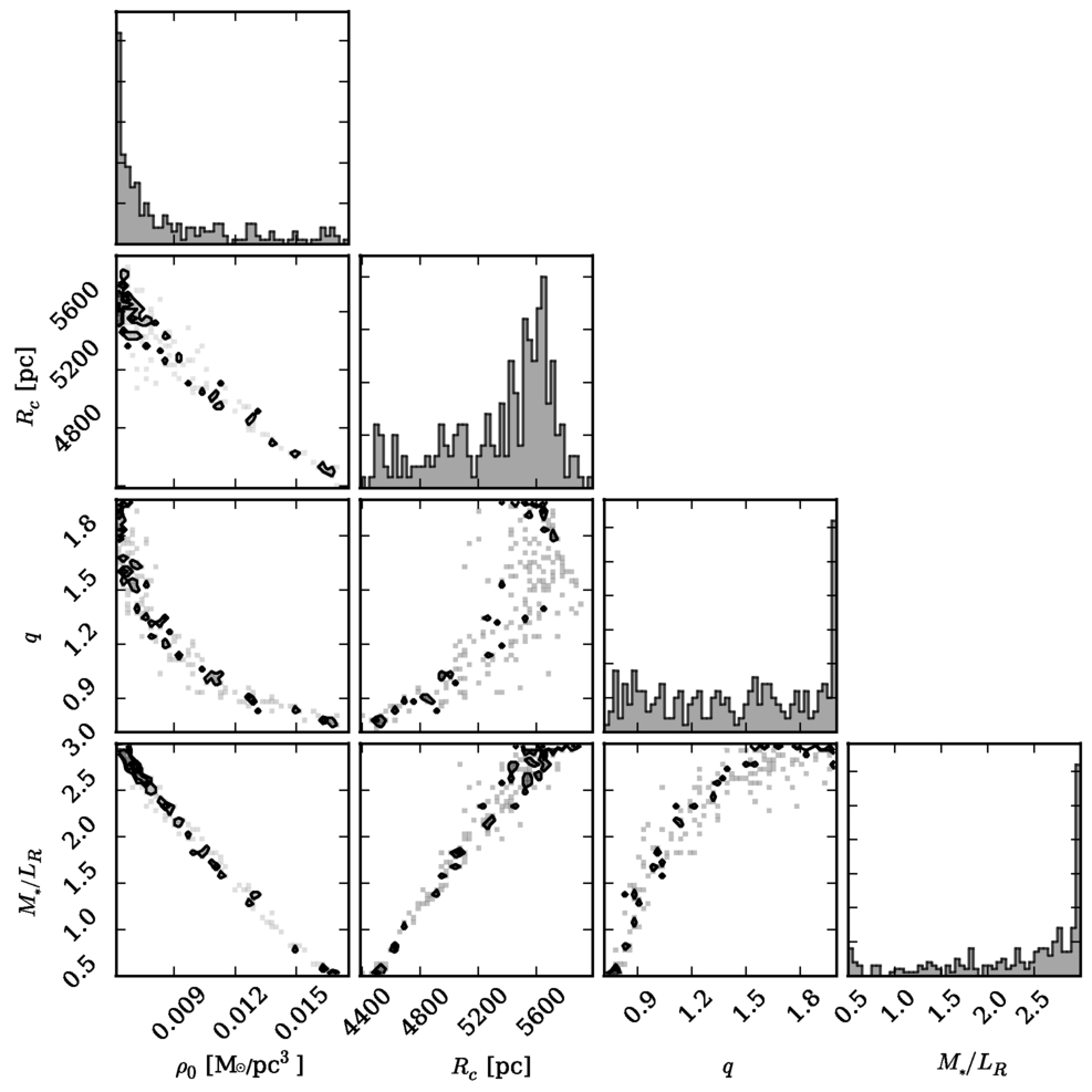
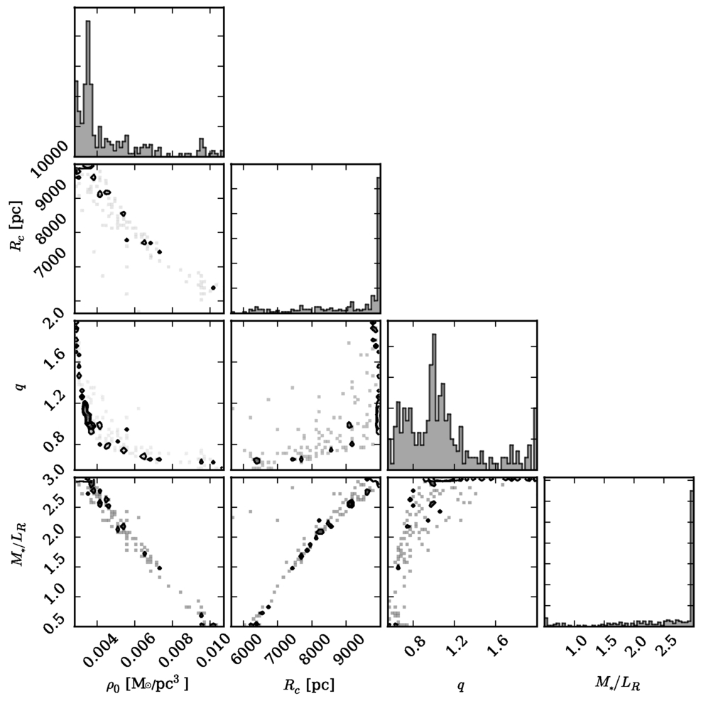
Figure 2: Correlation diagram for the optically thin model of IC 5249 (left) and the self-absorption model (right), both with a constraint of M/L$\geq 0.5$.

Figure 3: Rotation curve and vertical force gradient decomposition of ESO 115-G021. The left side panels show the results for the optically thin HI models, while the right side panels show the results for the self-absorption at $T_{\textrm{spin}}=100$ K results.

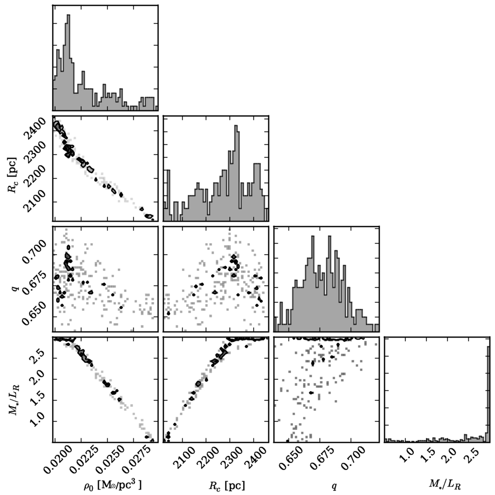
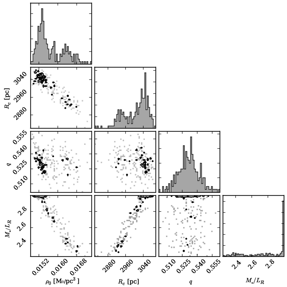
Figure 4: Correlation diagram for the optically thin model of ESO 115-G021 (left) and the self-absorption model (right), both with a constraint of M/L$\geq 0.5$.

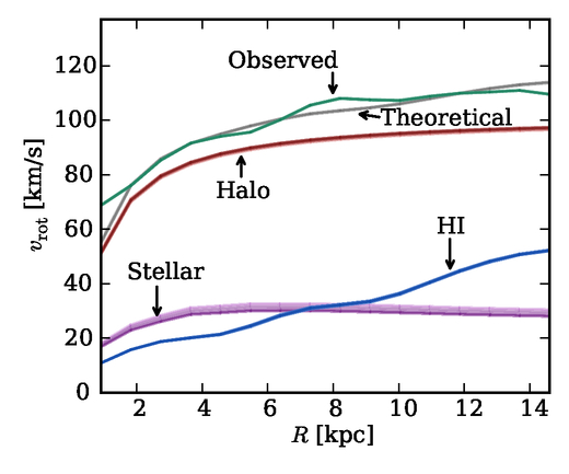
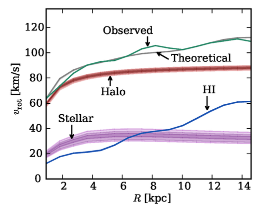
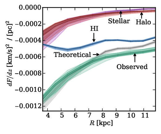
Figure 5: Rotation curve and vertical force gradient decomposition of ESO 138-G014. The left side panels show the results for the optically thin HI models, while the right side panels show the results for the self-absorption at $T_{\textrm{spin}}=100$ K results.

Figure 6: Correlation diagram for the optically thin model of ESO 138-G014 (left) and the self-absorption model (right), both with a constraint of M/L$\geq 0.5$.

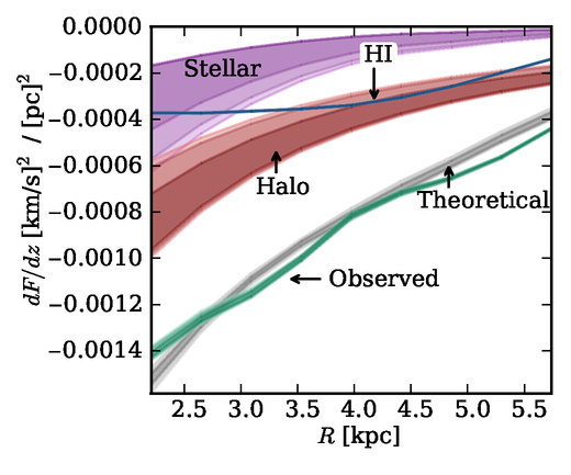
Figure 7: Rotation curve and vertical force gradient decomposition of ESO 274-G001. The left side panels show the results for the optically thin HI models, while the right side panels show the results for the self-absorption at $T_{\textrm{spin}}=100$ K results.

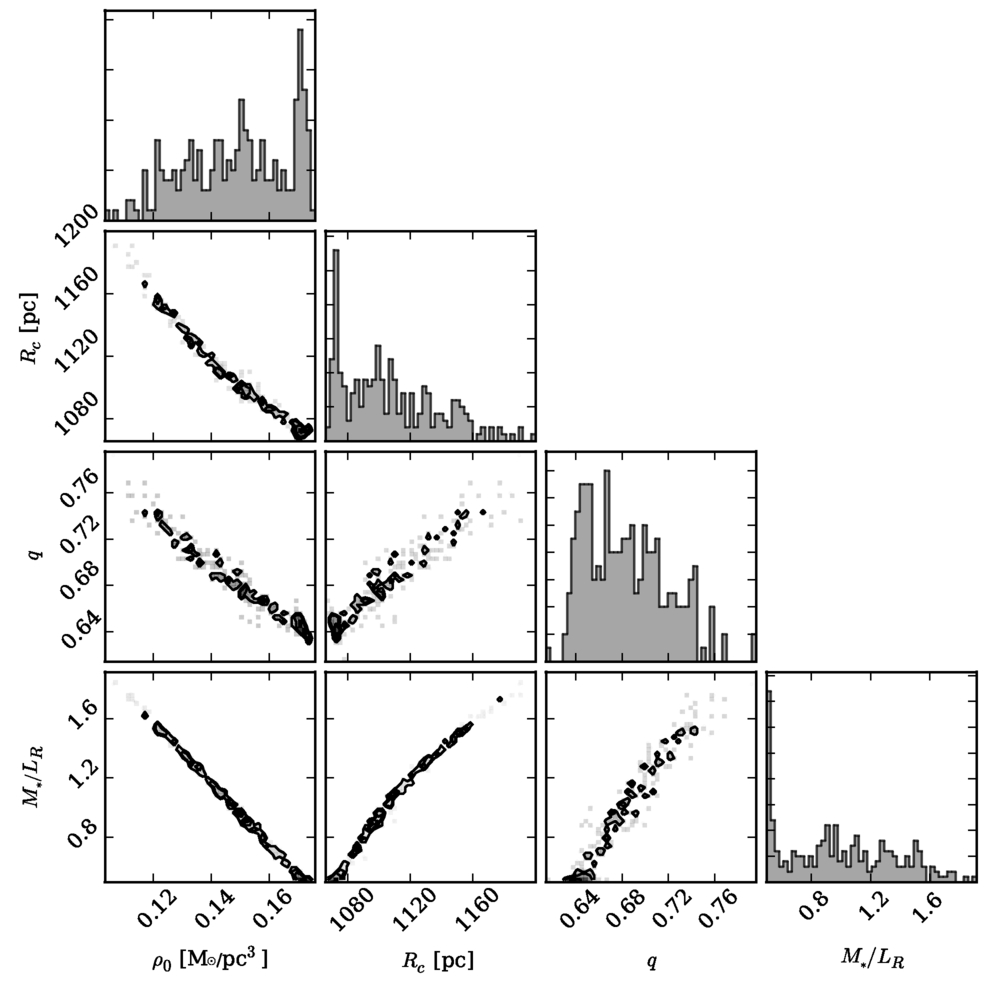
Figure 8: Correlation diagram for the optically thin model of ESO 274-G001 (left) and the self-absorption model (right), both with a constraint of M/L$\geq 0.5$.

3 Results

3.1 IC 5249

We have been moderately successful in modelling the dark matter halo of galaxy IC 5249. The decomposition of both the optically thin and self-absorbing HI results is shown in Figure 1. As is clear from the figure, the uncertainties in the stellar halo contribution, and subsequently the dark matter halo contribution are quite severe. This is mostly due to the fact that the measurements of both the vertical force gradient, as well as the rotation curve, start relatively far out (near 5.0-5.5 kpc). The data of the inward parts of the galaxy were too uncertain for a reliable measurement of the tracers. As the dark matter halo shape $q$ can most accurately be constrained from the vertical force gradient in the inner parts of the galaxy (see O’Brien et al., 2010), this lack of data does not allow us to constrain $q$ significantly. The optically thin HI model yields $q=1.5^{+0.5}_{-0.5}$, while the self-absorbing HI yields $q=1.0^{+0.4}_{-0.3}$.

The lack of a significant constraint on $q$ leads to strong correlations between the other parameters. This is reflected in the cross-correlation diagrams for the parameters, seen in Figure 2 (left) for the optically thin case, and Figure 2 (right) for the self-absorbing HI case. An oblate dark matter halo shape ($q<1$) produces a less massive stellar disc, with a shorter dark matter halo scale length $R_{c}$ and higher dark matter halo core density $\rho_{0}$. This behavior holds in both models. Over the whole dataset, we find that for an optically thin HI model the halo is found at $\rho_{0}=0.007^{+0.005}_{-0.001}$ M_⊙/pc³, $R_{c}=5.45^{+0.21}_{-0.52}$ kpc. The stellar disc is found with $M_{*}/L_{R}=2.62^{+0.38}_{-1.19}$. The self-absorption HI models return $\rho_{0}=0.004^{+0.003}_{-0.001}$ M_⊙/pc³, a scale length $R_{c}$ of $9.79^{+0.21}_{-2.06}$, and a stellar disc with $M_{*}/L_{R}=2.98^{+0.02}_{-1.17}$.

As we discussed in Section 2.1, the most likely $M_{*}/L_{R}$ values lie close to 0.5. If we thus limit ourselves to the data points at $M_{*}/L_{R}<0.55$, we find for the optically thin HI an oblate halo with $q=0.76_{-0.03}^{+0.04}$. The core density of the dark matter halo is $\rho_{0}=0.017_{-0.001}^{+0.001}$ M_⊙/pc³ and its scale length is $R_{c}=4.49_{-0.05}^{+0.02}$ kpc. The self-absorbing HI model returns an even more oblate halo, with a shape of $q=0.55_{-0.03}^{+0.14}$, a core density of $\rho_{0}=0.014_{-0.003}^{+0.003}$ M_⊙/pc³ and a scale length of $h_{0}=5.19_{-1.01}^{+1.30}$ kpc. Comparing the two models, we see that the dark matter halo of the self-absorbing HI requires a more oblate halo, with longer scale length $R_{c}$ and less massive central density $\rho_{0}$.

3.2 ESO 115-G021

We have not been very successful in modelling ESO 115-G021. As can be seen from the results in Figure 3, the observed vertical force gradient has a nearly flat slope near the inner parts of the galaxy ($R<4$ kpc). This is problematic to fit to, as we always expect the vertical force gradient to get increasingly strong near the inner parts. We have attempted fitting only beyond $R=3.5$ kpc, but this left only 2 kpc in which we could fit the data, which did not result in a stable fit. Smoothing was applied on the input parameters, but this did not improve the quality of the observed vertical force gradient. As such, we hereby present our best fit, but encourage the reader to have a skeptical treatment of them.

The self-absorbing HI model of the galaxy results in a dark matter core density $\rho_{0}$ of $0.015^{+0.001}_{-0.001}$ M_⊙/pc³, a scale length $R_{c}$ of $3.02^{+0.03}_{-0.08}$ kpc and an oblate shape of $q=0.5^{+0.1}_{-0.1}$. The stellar disk is found to have a high $M_{*}/L_{R}=2.89^{+0.11}_{-0.44}$. The optically thin HI model produces a more massive central core density $\rho_{0}=0.022^{+0.004}_{-0.001}$ M_⊙/pc³, a shorter scale length of $R_{c}=2.30^{+0.10}_{-0.15}$ and a less oblate halo shape $q=0.7^{+0.1}_{-0.1}$. We again find a high $M_{*}/L_{R}=2.84^{+0.16}_{-1.15}$
The cross-correlation diagrams of the models are shown in Figure 4.

3.3 ESO 138-G014

Galaxy ESO 138-G014 was initially hard to model, as the total observed vertical force gradient was already weaker than the contribution from the neutral hydrogen alone. As we noted before in Paper III, the galaxy seems to have quite a thick HI layer (see Figure 13 of Paper III). The most likely explanation for this is that the galaxy is not seen completely edge-on. This is consistent with the observed stellar disc from Paper IV, where we measured $i=86.8^{\circ}$ (Table 2 of Paper IV). We have attempted to correct for this by lowering the observed thickness by 30%, but will treat the results are uncertain in view of this inclination issue. The noise in this galaxy was too high for the velocity dispersion to be measure, so we keep this fixed at $\sigma=10$ km/s.

The results for the optically thin and the self-absorbing HI models are shown in Figure 5. The cross-correlation diagram of the optically thin model is shown in Figure 6 (left), while the one for the self-absorption model is shown in Figure 6 (right). In both cases, the rotation curve and the vertical force gradient have been successfully fitted. Only at the larger radii do observed and theoretical curves of the vertical force gradient start to deviate.

The optically thin model produces a halo core density $\rho_{0,\textrm{halo}}$ of $0.261^{+0.002}_{-0.003}$ M_⊙/pc³ and a scale-length of $R_{c}=0.70^{+0.02}_{-0.01}$ kpc. The halo is distinctly prolate, with the optimal solution located at the boundary condition of $q=2.0^{+0.1}_{-0.2}$. The stellar disc is very bright, with $M_{*}/L_{R}=0.50^{+0.02}_{-0.01}$.

Compared to this, the self-absorbing HI model finds a halo with a higher core density of $\rho_{0,\textrm{halo}}=0.620^{+0.009}_{-0.007}$ M_⊙/pc³ and a scale-length of $R_{c}=0.41_{-0.01}^{+0.02}$ kpc. Again, the optimal solution favors a prolate halo at $q=1.9^{+0.1}_{-0.3}$. In this case the mass-to-light is $M_{*}/L_{R}=0.69^{+0.04}_{-0.06}$.

3.4 ESO 274-G001

Galaxy ESO 274-G001 is one of the two galaxies from Paper III for which we could accurately measure the velocity dispersion. We model the galaxy in the standard way, setting the $M_{*}/L_{R}$ lower boundary at 0.5. Both the rotation curve and vertical force decomposition are shown in Figure 7, where we show the results for both the optically thin and self-absorbing HI models. Both models have reproduced the rotation curve and the vertical force gradient reasonably well, although the self-absorbing model was more successful at the vertical force gradient.

We show the cross-correlation diagram for the optically thin HI model in Figure 8 (left). There is a clear correlation between the various parameters, which is mostly due to the uncertainty in $M_{*}/L_{R}=0.96^{+0.46}_{-0.42}$. The halo is oblate with $q=0.7^{+0.1}_{-0.1}$, $\rho_{0,\textrm{halo}}=0.150^{+0.020}_{-0.022}$ M_⊙/pc³ and $R_{c}=1.10^{+0.04}_{-0.03}$ kpc. The mass to light ratio $M_{*}/L_{R}$ was $0.96^{+0.46}_{-0.42}$.

The cross-correlation diagram of the HI self-absorption model is shown in Figure 8 (right). There is again scatter in $M_{*}/L_{R}$, although the value has dropped compared to the optically thin model. It is now at $0.76^{+0.57}_{-0.26}$. The shape of the halo is identical to the optically thin model, with an oblate shape of $q=0.7^{+0.1}_{-0.1}$. The other parameters are $\rho_{0,\textrm{halo}}=0.094^{+0.009}_{-0.019}$ M_⊙/pc³ and $R_{c}=1.42^{+0.09}_{-0.03}$ kpc. Compared to the optically thin model, the self-absorption HI model produces a dark matter halo with longer scale length $R_{c}$ and lower central density $\rho_{0}$.

If we limit the analysis to $M_{*}/L_{R}<0.55$, we find that the halo becomes even more oblate, $q=0.64_{-0.01}^{+0.01}$ for the optically thin and $q=0.67_{-0.01}^{+0.01}$ for the self-absorption model. The central density of the halo also goes up to $\rho_{0}=0.171_{-0.001}^{+0.002}$ M_⊙/pc³ for the optically thin model, and $\rho_{0}=0.103_{-0.001}^{+0.001}$ M_⊙/pc³ for the self-absorbing HI . The scale lengths goes down to $h_{0}=1.07_{-0.01}^{+0.01}$ kpc and $h_{0}=1.39_{-0.01}^{+0.01}$ kpc respectively. A lower mass in the stellar disc thus results in haloes that are more oblate, have higher central core densities and slightly shorter scale lengths.

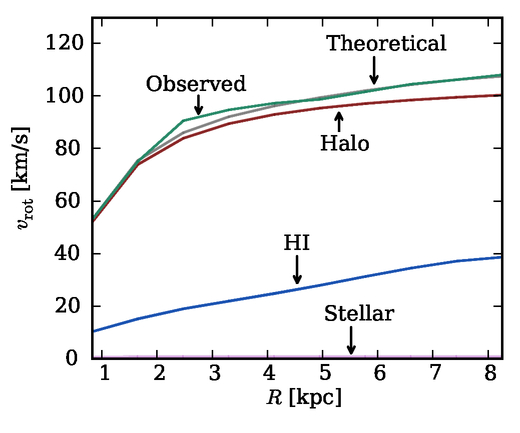
Figure 9: Rotation curve decomposition of UGC 7321 for various models. From top-left to bottom-right: optically thin HI (M/L $\geq 0$), optically thin HI (M/L $\geq 0.5$), self-absorption HI (M/L $\geq 0$), self-absorption HI (M/L $\geq 0.5$), spherical halo with self-absorption HI (M/L $\geq 0$), spherical halo with self-absorption HI (M/L $\geq 0.2$)

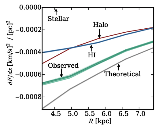
Figure 10: Vertical force decomposition of UGC 7321 for various models. From top-left to bottom-right: optically thin HI (M/L $\geq 0$), optically thin HI (M/L $\geq 0.5$), self-absorption HI (M/L $\geq 0$), self-absorption HI (M/L $\geq 0.5$), spherical halo with self-absorption HI (M/L $\geq 0$), spherical halo with self-absorption HI (M/L $\geq 0.5$)

Figure 11: Correlation diagram for the optically thin model of UGC 7321 (left) and for the self-absorption model (right), both with a constraint of M/L$\geq 0.5$.

3.5 UGC 7321

Galaxy UGC 7321 has the highest signal to noise ratio for the HI data from our sample. The galaxy was previously modelled by O’Brien et al. (2010), who found that the halo flattening $q$ was round ($q=1.0\pm 0.1$). Their modelling strategy consisted of a two-pass scheme, in which they first performed a rotation curve decomposition, and only then performed a separate fit to the vertical force gradient. This second fit however failed, and the authors had to drastically deviate from the results from the rotation curve decomposition, and use a very low mass stellar disc, in order to reproduce the observed vertical force gradient. We have performed an inspection of the codes used by in the analysis of O’Brien et al. (2010). It appears there was a restriction which allowed only models with $q\leq 1$ and it would have been impossible for them to fit a prolate halo.

Banerjee et al. (2010) also analysed UGC 7321 and found a spherical halo. These authors assumed a constant velocity dispersion, or at most a decreasing gradient, in their work, and use a different potential than us.

In Figure 9, we demonstrate our own rotation curve decomposition of this galaxy, and in Figure 10 we show the vertical force gradient decomposition. Rather than present decompositions for only the optically thin and self-absorbing HI models that we measured, as for the previous galaxies, we show the results for six fits.

Since O’Brien et al. (2010) found a good fit at a negligible stellar mass, the first panel in both figures demonstrates a fit in which the $M_{*}/L_{R}$ can range between zero and three, for an optically thin HI disc. This fit should therefore be the closest to the results obtained by O’Brien et al. (2010). The 1000 samples produce a range of solutions. Both the rotation curve and the vertical force gradient are well reproduced. The mass-to-light ratio has a median of $M_{*}/L_{R}=1.58_{-0.68}^{+0.45}$, which is significantly higher than measured by O’Brien et al. (2010). The halo is very prolate, $q=1.90_{-0.32}^{+0.10}$ and has a high central density of $\rho_{0,\textrm{halo}}=0.324_{-0.043}^{+0.067}$ M_⊙/pc³ and short scale-length of $R_{c}=0.64_{-0.02}^{+0.05}$ kpc. Previously, O’Brien et al. (2010) have reported $R_{c}=0.52\pm 0.02$ kpc and $\rho_{0,\textrm{halo}}=0.73\pm 0.05$ M_⊙/pc³.

As we estimate a minimum of $M_{*}/L_{R}=0.5$, the second panel raises the boundary condition for the minimal stellar mass-to-light ratio to $0.5$. The mass-to-light is found to be $M_{*}/L_{R}=1.63_{-0.66}^{+0.48}$, still very similar to the previous model. The observed rotation curve and vertical velocity gradients are well reproduced, as shown in Figures 9 and 10. We find $\rho_{0,\textrm{halo}}=0.318_{-0.042}^{+0.064}$ M_⊙/pc³ and $R_{c}=0.64_{-0.02}^{+0.03}$ kpc, roughly similar values as the previous fit. The halo shape runs firmly towards $q=2$, which is also the boundary condition. We have tested the effect of lifting this boundary condition. When we do this, the model tends to run towards even greater values of $q$. However, since the current research question focuses primarily on prolate versus oblate, we have decided to stick to an upper boundary of $q=2$. We present a cross correlation diagram of this fit in Figure 11 (left).

Our next fit uses the self-absorption HI model rather than the optically thin model. We again let $M_{*}/L_{R}$ run from zero to three. As shown in Figures 9 and 10, the stellar disc in this fit gets a negligible mass assigned ($M_{*}/L_{R}=0.00_{-0.00}^{+0.04}$). The other parameters are $\rho_{0,\textrm{halo}}=0.307_{-0.003}^{+0.002}$ M_⊙/pc³, $R_{c}=0.71_{-0.01}^{+0.01}$ kpc and $q=1.84_{-0.09}^{+0.12}$. Compared to the optically thin model, the dark matter halo is again strongly prolate, but has a longer scale-length and lower central density.

Similar to the optically thin HI case, we again increase the lower $M_{*}/L_{R}$ boundary to $0.5$. The results are shown in Figures 9 and 10. The observed rotation curve has been modelled well, but the model fails to account for the vertical force gradient and produces too strong a vertical force gradient. This directly illustrates why $M_{*}/L_{R}$ was zero in the previous fit, as this was the only way for the vertical force gradient to be fit. The parameters found are $\rho_{0,\textrm{halo}}=0.28_{-0.01}^{+0.01}$ M_⊙/pc³, $R_{c}=0.72_{-0.01}^{+0.01}$ kpc, $q=2.00_{-0.03}^{+0.01}$ and $M_{*}/L_{R}=0.5$. The cross-correlation diagram for this fit is shown in Figure 11 (right).

In their revious study, O’Brien et al. (2010) were unable to fit the rotation curve and the vertical force gradient simultaneously. They successfully started with a rotation curve decomposition, in which the stellar disc mass was a free parameter. However, in order to subsequently perform their vertical force gradient decomposition, they were forced to drastically lower the stellar mass. They eventually found a spherical halo, but only when they allowed very small $M_{*}/L_{R}$ (the best fit was actually for $M_{*}/L_{R}=0$), smaller than we allowed here.

As two final tests, we ran fits to the optically thin and self-absorption HI results, in which we constrained $q=1$. The results are shown in Figures 9 and 10. The rotation curve decomposition does not depend strongly on $q$ (O’Brien et al., 2010). As such, it is again reproduced well. Clearly, however, the vertical force gradient is fit poorly. A spherical halo simply does not work for this galaxy.

Name	HI model	$\rho_{0}$ [M⊙/pc3]	$R_{c}$ [kpc]	$q$	$M_{*}/L_{R}$
IC 5249	SA	$0.004^{+0.003}_{-0.001}$	$9.79^{+0.21}_{-2.06}$	$1.0^{+0.4}_{-0.3}$	$2.98^{+0.02}_{-1.17}$
IC 5249	OT	$0.007^{+0.005}_{-0.001}$	$5.45^{+0.21}_{-0.52}$	$1.5^{+0.5}_{-0.5}$	$2.62^{+0.38}_{-1.19}$
ESO 115-G021	SA	$0.015^{+0.001}_{-0.001}$	$3.02^{+0.03}_{-0.08}$	$0.5^{+0.1}_{-0.1}$	$2.89^{+0.11}_{-0.44}$
ESO 115-G021	OT	$0.022^{+0.004}_{-0.001}$	$2.30^{+0.10}_{-0.15}$	$0.7^{+0.1}_{-0.1}$	$2.84^{+0.16}_{-1.15}$
ESO 138-G014	SA	$0.620^{+0.009}_{-0.007}$	$0.41^{+0.02}_{-0.01}$	$1.9^{+0.1}_{-0.3}$	$0.69^{+0.04}_{-0.06}$
ESO 138-G014	OT	$0.261^{+0.002}_{-0.003}$	$0.70^{+0.02}_{-0.01}$	$2.0^{+0.1}_{-0.2}$	$0.50^{+0.02}_{-0.01}$
ESO 274-G001	SA	$0.094^{+0.009}_{-0.019}$	$1.42^{+0.09}_{-0.03}$	$0.7^{+0.1}_{-0.1}$	$0.76^{+0.57}_{-0.26}$
ESO 274-G001	OT	$0.150^{+0.020}_{-0.022}$	$1.10^{+0.04}_{-0.03}$	$0.7^{+0.1}_{-0.1}$	$0.96^{+0.46}_{-0.42}$
UGC 7321	SA	$0.270^{+0.001}_{-0.001}$	$0.72^{+0.01}_{-0.01}$	$2.0^{+0.1}_{-0.1}$	$0.50^{+0.02}_{-0.01}$
UGC 7321	OT	$0.318^{+0.064}_{-0.042}$	$0.64^{+0.03}_{-0.02}$	$1.9^{+0.1}_{-0.3}$	$1.63^{+0.48}_{-0.66}$

Table 1: Measured parameters for the various haloes. OT denotes the optically thin HI models, while SA denotes the self-absorbing HI models.

In the previous section, we have presented the results for the individual galaxies. So how do the results compare to each other? In Table 1, we present an overview of all the derived parameters. For ESO 138-G014, we only present the results where the thickness of the HI layer has been reduced by 30%. For galaxy UGC 7321, we present the results for the default model, in which the mass-to-light ratio $M_{*}/L_{R}$ was allowed to vary between 0.5 and 3.0, and the halo shape $q$ between 0.1 and 2.0.

We present an overview of the average of these parameters in Table 3. There is an interesting difference between optically thin and self-absorbing HI models. Overall, we see that the halo of an optically thin HI model has a core density that is overestimated by $150\%$. The scale length of the dark matter halo is $28\%$ longer in the self-absorption model, compared to the optically thin model. In addition, where the optically thin models have a median shape that is prolate, the median shape is spherical in self-absorption HI models. The mass-to-light ratio of the stellar disc drops by more than half when self-absorbing HI is accounted for.

All of our five discs are sub-maximal. This was already demonstrated by O’Brien et al. (2010) and Banerjee et al. (2010) for UGC 7321, who reported a stellar disc M/L_R at a maximum of 2.5, although their final decomposition found a maximum of M/L_R = 0.2. The result is consistent with the work by Bershady et al. (2011), who argued that all galaxies are sub-maximal based on an analysis of the central vertical velocity dispersion of the discs stars and the maximum rotation of 30 face-on galaxies. Similar conclusions have previously been reached by Bottema (1997) and Kregel et al. (2005). Martinsson et al. (2013a) confirmed these results after performing dynamically determined rotation curve mass decompositions for all these 30 galaxies.

Name	$\rho_{0}$ [M⊙/pc3]	$R_{c}$ [kpc]	$q$	$M_{*}/L_{R}$	Citation
UGC 7321	$0.73\pm 0.05$	$0.52\pm 0.02$	$1.0\pm 0.1$	$0.2$	O’Brien et al. (2010)
UGC 7321	$0.048\pm 0.009$	$2.7\pm 0.2$	1		Banerjee et al. (2010)
NGC 4244	$0.6595\pm 0.6495$	$6.15\pm 5.85$	0.2		Olling (1996)
M 31	0.011	21	0.4		Banerjee & Jog (2008b)
Galaxy (NFW)	$0.0413_{-0.016}^{+0.013}$	$9.26_{-4.2}^{+5.6}$			Nesti & Salucci (2013)
Galaxy	$0.0147_{-0.0093}^{+0.029}$	$16.1_{-7.8}^{+17}$			Nesti & Salucci (2013)
Galaxy		12	5/3		Helmi (2004)
Galaxy		7.1	0.7		Olling & Merrifield (2000)
Lensing		$23.9_{-0.5}^{+0.2}$	$0.62_{-0.25}^{+0.25}$		van Uitert et al. (2012)
ESO 138-G014 (NFW)	$0.013\pm 0.002$	$7.5\pm 0.5$			Hashim et al. (2014)
ESO 138-G014 (Burkert)	$0.077\pm 0.042$	$10.7\pm 2.7$			Hashim et al. (2014)

Table 2: Overview of haloes measured in other papers that were used in Figure 12 as data points.

In Figure 12, we demonstrate the correlation between the four free parameters from our fit. We have also included a range of points from other authors in this view (see Table 2 for an overview, note that multiple halo models are used an as such the core radius can be expected to vary). Inspecting the figure, the most notable correlations is the one between core radius $R_{c}$ and halo core density $\rho_{0}$. With the exception of one point, ESO 138-G14 by Hashim et al. (2014) using a NFW halo, all of the points seem to follow a relation of $R_{c}\approx 1/\rho_{0}$. Our result for ESO 138-G14 are uncertain due to the possiblity of a r4esisual inclination compared to edge-on and any results on this galaxy, including ours at $q\sim 2$ should be treated with caution. This relation is similar to the degeneracy between the two parameters in an individual galaxy, as for example in Figure 11, and it interesting to observe a similar trend visible across multiple galaxies and halo models. If this is a true relation, then it implies that there are two families of haloes: one compact halo family with high core density $\rho_{0}$ and scale length $R_{c}$, and a second non-compact halo family with low core density $\rho_{0}$ and scale length $R_{c}$.

name	optically thin	self absorbing
$\rho_{0}$	$0.150\pm 0.124$	$0.094\pm 0.230$
$R_{c}$	$1.10\pm 1.81$	$1.42\pm 3.48$
$q$	$1.5\pm 0.6$	$1.0\pm 0.6$
$M_{*}/L_{R}$	$1.63\pm 0.91$	$0.76\pm 1.12$

Table 3: Overview of the global parameters of our halo sample. Shown are the median and standard deviations of the parameters. The units of $\rho_{0}$ are in M_⊙/pc³ and those of the radius $R_{c}$ in kpc.

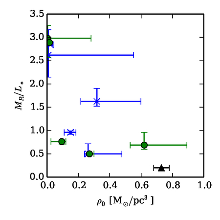
Figure 12: Overview of the correlations between the various halo parameters. Blue crosses represent the halo parameters for the self-absorbing HI , while green circles represent the optically thin models. Black markers are the data points from Table 2

Our best results are for ESO 274-G001 and UGC 7321, where we have been able to include a measurement of the velocity dispersion of the HI as function radius in the analysis. Focusing on these two, we find two very different haloes. In ESO 274-G001, the halo is oblate with a shape $q=0.7\pm 0.1$ (regardless of the HI model); while in UGC 7321, the halo is distinctly prolate with a shape of $q=1.9^{+0.1}_{-0.3}$ (optically thin HI ) and $q=2.0\pm 0.1$ (self-absorbing HI ).

So how do these shapes compare to other galaxies? Looking at our own Galaxy, Law & Majewski (2010) propose a triaxial dark matter halo for the Milky Way, in which $(c/a)_{\phi}=0.72$ and $(b/a)_{\phi}=0.99$. Banerjee & Jog (2011) proposed a dark matter halo shape for the Galaxy which becomes progressively more prolate with radius. Vera-Ciro & Helmi (2013) report an oblate halo with $q=0.9$ for the inner 10 kpc, based on stellar streams. Using lensing, Barnabè et al. (2012) also found a slightly oblate halo at $q=0.91^{+0.15}_{-0.13}$ for galaxy SDSS J2141. The large weak lensing galaxies sample of van Uitert et al. (2012), in which $2.2\times 10^{7}$ galaxies were studied, produced a halo ellipticity distribution that also favors oblate haloes. The distributions of the halo shape $q$ was $0.62^{+0.25}_{-0.25}$. The three polar ring galaxies studied by Whitmore et al. (1987), A0136-0801, NGC 4650A and ESO 415-G026, had slightly oblate to spherical halo shapes $q$: $0.98\pm 0.20$, $0.86\pm 0.21$ and $1.05\pm 0.17$. From this selected sample of papers, it becomes apparent that our result for ESO 274-G001, with $q=0.7\pm 0.1$, is consistent with other papers.

While ESO 274-G001 clearly matches up with measurements in other galaxies, the other case of our two best fits, UGC 7321, is a more ‘problematic’ one (Figures 13, 14, 15 and 16). With a halo shape of $q=1.9_{-0.3}^{+0.1}$ for the self-absorption model, the dark matter halo shape is very strongly prolate. As we commented before in Section 3.5, our upper boundary condition for the halo shape is $q\leq 2$. If we had removed this boundary, some of the fits returned results as high as $q\sim 5000$, which are clearly not physical. The galaxy has been previously analysed by Banerjee et al. (2010), whom successfully modelled the dark matter halo shape for a spherical halo. O’Brien et al. (2010) had problems fitting the dark matter halo shape. They had to lower their initially measured asymptotic halo rotation (see Equation 20) in order to get a successful fit to their data at $q=1.0\pm 0.1$, although they were limited to $q\leq 1$ in their analysis. Had their boundary condition been higher, it would have been likely that they too would have found higher values for $q$.

3.6 Concerns regarding reliability and degeneracy

Given that our two best galaxies produce such drastically different results, how reliable is our methodology? To answer this question, let us recap the underlying assumptions from this paper and Paper IV.

3.6.1 Concerning the neutral hydrogen

We start with the neutral hydrogen. In Paper I, we argued that the HI in edge-on galaxies could suffer from significant self-absorption. To model the HI more accurately, we developed a new tool that allowed the neutral hydrogen in galaxies to be fit automatically, while incorporating a treatment for the self-absorption of the gas. Indeed, we saw in Section 7 of Paper II that the visible mass of a galaxy drops as one rotates it from face-on to fully edge-on. In Paper II, we developed a method to model the HI content of a galaxy that was edge-on. In Section 3 of Paper III, we tested this method on a series of simulated galaxies, showing that we could reproduce the input parameters reasonably well using our method. We also demonstrated that assuming an optically thin HI disc, which in reality was self-absorbing, could lead to a wrong measure of face-on surface density, thickness of the HI layer and the velocity dispersion. We have continued the use of the optically thin HI results into this paper to demonstrate how the dark matter halo measurement is affected by this. As discussed in the previous section, the results are drastic. How accurate are our results now?

One of the key assumptions made in Paper II was the effective spin temperature of the neutral hydrogen of $100$ K. While this was has proven a very successful value on which to base our results, it is an assumption based purely on what seemed to work best. In reality the neutral hydrogen most likely consists of multiple phases, such as the cold neutral medium (CNM) and warm neutral medium (WNM). The effective spin temperature is a result of the mix of the phases of the CNM, which has a median spin temperature of 80 K and the WNM, with temperatures between 6000 and 10000 K. In Section 4 of Paper II, we demonstrated how the interplay of HI gas phases could lead to an effective median spin temperature. So what would be the consequence of a wrong estimate of the spin temperature? Suppose that the spin temperature would have been $T_{\textrm{spin}}=90$ K rather than 100 K. In that case the face-on surface density of the neutral hydrogen will be higher, which in this paper would lead to higher theoretical rotation from the gas components in the galaxy and stronger vertical force gradients then are currently found. Simultaneously, the thickness of the disc would be smaller, and thus the total observed vertical force gradient would be larger (Equation 9). Although hard to estimate the exact effect, the phases of the HI all have different distributions, together producing the observed thickness of the disc (Lockman & Gehman, 1991). The effective spin temperature could thus be height dependent as well.

Another assumption is the uniform density of the HI as a function of radius. In reality of course, galaxies have spiral arms, supernova, shocks, gravitational collapse, and other features, all of which create a drastically non-uniform HI disc. The question thus remains how strongly the parameters are affected by this. Kamphuis et al. (2013) made a valiant attempt to model the density waves in galaxies NGC 5023 and UGC 2082, demonstrating that these could be detected in edge-on galaxies. Indeed, as we discussed in Section 5 of Paper I, the position-velocity (XV-)diagrams are not symmetric on both side of the galaxies. This problem would most strongly affect the velocity dispersion, which is dependent upon small-scale features. In most cases, this leads to an overestimation of the HI velocity dispersion, as the fitting algorithm tries to ‘smooth over’ the small-scale fluctuations. The result would be an overestimation of the observed vertical force gradient through Equation 9. This could be a likely reason why UGC 7321 has such a distinctive halo shape.

We have also assumed that the HI has an isotropic velocity dispersion tensor, i.e has the same value in the $R$, $z$ and $\theta$ directions (see Section 2.2 of Paper II). While there currently is no observational proof that this is an invalid assumption, it remains untested. If the velocity dispersion tensor were in reality anisotropic, it would imply that our observed vertical force gradient is wrong (Equation 9). Simultaneously, it would affect the amount of observed HI in the self-absorption mode, as gas with low velocity dispersion would give a alrger effect than gas with high velocity dispersion (Equation 19 of Paper II). It would affect the rotation curve measurements to a minor degree.

We also have assumed that the velocity dispersion is isothermal in $z$, i.e. does not vary with height. In Section 4.7 of Paper III, we have attempted to measure this in ESO 274-G001. We found a very small increase of 1 km/s in the slice above the central 290 pc of the disc. If this were confirmed in other galaxies, it would mean that Equation 8 is false, and thus our observed total force gradient would have been wrong. Previously, Lockman & Gehman (1991) has attempted to model the vertical structure of the Galaxy using multiple HI phases, which had different scale heights and velocity dispersions. The phases with the highest scale heights also have the highest velocity dispersions. It is quite possible that the effective spin temperature of the different phases would increase for those with larger scale heights. Assuming that our currently observed velocity dispersion is due to the combination of high and low $z$ gas, the total vertical force gradient than we are currently reporting would be weaker in the mid-plane, and stronger at high values of $z$.

The thickness of the HI disc has been assumed to follow a Gaussian form (see Equation 15 of Paper II) for mathematical convenience in Equation 9. Other possible candidates for the HI model would have been the sech and sech² functions. Olling (1995) previously discussed the various types of discs and concluded that the changes due to this would be minor. A sech function has more extended wings and steeper inner slopes, compared the Gaussian function. If our galaxies have high-projected latitude gas, such as due to warps or HI haloes, then it is possible that a fit with a Gaussian function would find the FWHM of the disc to be unrealistically large. A fit with a sech or even sech² function could then be a better approximation to the shape of the HI disc.

Another assumption in our model is the perfect edge-on nature of the HI disc. In Section 3.5 of Paper III, we tested how our HI fitting strategy worked on a galaxy at $i=88.8^{\circ}$. We found that the parameters were well recovered. However, suppose that some galaies are even further from edge-on than that, as formally indicated by our stellar decompositions (Table 4 of Paper IV). In that case, the thickness of the HI is probably overestimated and the circular rotation underestimated. This has a profound effect on the rotation curve decomposition, which would require a larger rotational contribution due to the dark matter. In a similar vein, the total observed vertical force gradient would be underestimated, and would thus require a more massive dark matter halo in the decomposition. On the other hand, the density of the HI would be lower at a height of 100 pc, such that in Equation 10 the vertical force gradient due to the HI would be lower.

3.6.2 Concerning the stellar disc

In Paper IV, we set out to use the FitSKIRT tool to model the stellar disc of our sample of galaxies. We modelled the galaxies using a stellar disc and a bulge component. While the results were acceptable in most cases, these galaxies were selected to be relatively bulge-less (Section 3 of Paper I). Because of this, the fitting routine was found to ‘misuse’ the bulge component as a tool to better model the stellar disc. Thus, the bulges in most of the galaxies serve more like an extension of the stellar disc, rather than like a separate central component (see Table 4 of Paper IV for the parameters). In some cases, the amount of light from the bulge component is similar to that of the stellar disc itself (Table 3 of Paper IV). Due to the massive amount of processing power required to perform the stellar decompositions, we have been unable to test how well the fitting of just an exponential disc to the data would have worked. Most likely, the results are similar to the combined parameters adopted here.

The stellar models in Table 4 of Paper IV were often found to deviate from complete edge-on. In the absence of dust lanes, which could prove an independent check, it remains unclear how accurate this result is. If the galaxies were in reality more edge-on than measured, the stellar discs would have shorter scale heights. In Equation 10, this would imply a lower stellar density at a height of $z=100$ pc, and thus would require a stronger dark matter halo vertical force gradient.

3.6.3 Concerning the cross-correlation between parameters

An advantage of our MCMC method is that we have not one, but a whole range of parameter sets for each galaxy. This allows us to explore the interplay between the cross-correlations, such as demonstrate Figure 12 for the self-absorption model of ESO 274-G001. As is clear from this figure, a whole range of solutions can be valid. For example, one parameter set returned a core density of 0.1 M_⊙/pc³, with scale length of 1.4 kpc, halo shape $q$ of $0.67$ and $M_{*}/L_{R}$ of 0.4. A different but equal parameter set returned a core density of $0.06$,M_⊙/pc³, with scale length of nearly 1.6 kpc, shape $q=0.84$ and $M_{*}/L_{R}$ of 1.7. These results are drastically different, yet both are accepted parameter sets.

The largest source of uncertainty is the stellar disc $M_{*}/L_{R}$. It was beyond the scope of this project to measure this parameter in each of our galaxies, which is why we have adopted it as a free parameter. A different solution would have been to adopt the maximum value of $M_{*}/L_{R}$ permitted in the rotation curve decomposition, the so-called maximum disc approach (e.g. Carignan & Freeman (1985); van Albada et al. (1985)). However, these galaxies were selected to be dark matter dominated at all radii and as such this approach would have been invalid (Section 3 of Paper I). In addition, the applicability of the maximum disc criteria has already been questioned by Kregel et al. (2005) and Martinsson et al. (2013b), whom both report sub-maximal stellar discs. Although beyond the scope of this project, the best approach would be to perform a full stellar population synthesis analysis of each galaxy. For examples see Bruzual & Charlot (2003) and Maraston (2005). By measuring M_⊙/pc³ rather than using it as a free parameter, the solution space becomes far less degenerate and the parameters can thus be fixed far more accurately.

Another cause of concern is the boundary conditions imposed upon our data. We have done our best to impose realistic boundary conditions. For the dark matter halo shape, we adopted $0.1<q<2.0$, as we believe that even more oblate or prolate haloes would be unrealistic. In Section 2.1 we adopted $0.5<M_{*}/L_{R}<3.0$ as a likely boundary, based on the stellar population models by Worthey (1994) and Bertelli et al. (1994). As can clearly be seen from the various cross-correlation diagrams, the models often still run into the boundary conditions. While it is possible to raise or remove the boundary conditions, we do not believe that this would lead to realistic results and we have therefore refrained from doing so.

3.6.4 Halo model

In this work, we have adopted the dark matter halo model by Sackett et al. (1994). With this model, we can create flattened, axi-symmetric, pseudo-isothermal haloes. In this model, the density is stratified in concentric ellipsoids. We have chosen this model to be able to compare directly to O’Brien et al. (2010), who also use this model.

There are many other halo model. Carignan & Freeman (1985, 1988) used isothermal, rather than pseudo-isothermal haloes to model their galaxies. Kormendy & Freeman (2004) compared the merits between isothermal and pseudo-isothermal haloes. As is shown in that paper (and reproduced in O’Brien et al., 2010), the rotation curve of an isothermal halo initially rises above the asymptotic velocity $v_{H}$, before dropping towards it again. In contrast, the pseudo-isothermal rotation curve approaches the asymptotic velocity gradually from lower values. This behavior would affect the results for the rotation curve decomposition.

There are more models, such as the NFW and Burkert halo model, each of which has some mathematical or theoretical advantage (Burkert, 1995; Navarro et al., 1996). Even more exotic models exist in which the dark matter halo shape can vary with radius (Vera-Ciro & Helmi, 2013). This can for example lead to haloes that get progressively more prolate with radius (Banerjee & Jog, 2011). While all these haloes are very interesting, we believe that the quality of the data, as discussed in this section, does not warrant such a detailed exploration of the properties of the various halo models.

An altogether different solution would have been the use of MOND, which would have removed the need for a dark matter halo altogether (Milgrom, 1983). We find that in many of our vertical force decompositions, a slight increase in the mass of the HI and stellar disc would be sufficient to account for the total observed vertical force gradient. As we argued before, additional mass in both the stellar and HI discs is allowed for by the data. While it is beyond the scope of this project to test MOND on our data, it is an interesting avenue for further research.

4 Conclusions

We have attempted to measure the shape of the dark matter halo in five galaxies, using a simultaneous decomposition of the rotation curve and of the vertical force gradient at the mid-plane. For a dark matter halo model, we have adopted the Sackett et al. (1994) dark matter halo. Both optically thin and self-absorbing HI models were used. We find that this leads to drastically different results. As we have argued in Papers I, II and III, the HI self-absorption models are the more accurate representation of galaxies. Using HI self-absorption, we found that a typical dark matter halo has a less dense core ($0.094\pm 0.230$ M_⊙/pc³) compared to an optically thin HI model ($0.150\pm 0.124$ M_⊙/pc³). The HI self-absorption dark matter halo had a longer scale length $R_{c}$ of $1.42\pm 3.48$ kpc, versus $1.10\pm 1.81$ kpc for the optically thin HI model. The median halo shape was spherical, at $q=1.0\pm 0.6$ (self-absorbing), while it was prolate at $q=1.5\pm 0.6$ for the optically thin.

Our best results were obtained for ESO 274-G001 and UGC 7321, for which we were able to measure the velocity dispersion in Paper III. These two galaxies have drastically different halo shapes. ESO 274-G001 was found to be oblate at $q=0.7\pm 0.1$ (both HI models), while UGC 7321 returns a distinctly prolate halo at $q=1.9_{-0.3}^{+0.1}$ (optically thin) and $q=2.0\pm 0.1$ (self-absorbing). The halo of ESO 274-G001 iss similar to those found in other studies, but UGC 7321 is more problematic. In UGC 7321, the most likely cause of concern is the presence of spiral arms and an HI halo.

With these drastically different results, we concluded that the question whether haloes are oblate or prolate is not settled. The results for both of our best galaxies appear to be fine. A larger set of galaxies needs to be analysed, before it can become clear if one of these galaxies is an outlier, or if prolate and oblate haloes are equally likely in nature.

We extensively discussed the various assumptions and sources of uncertainty in our models, of which there are many. While we have done our best to treat for these assumptions, for example using MCMC fits to the HI cube, we found that fitting the hydrostatics of the dark matter halo using the vertical force gradient near the mid-plane of the galaxy will always be tricky.

References

- Banerjee & Jog (2008a) Banerjee A., Jog C. J., 2008a, ApJ, 685, 254
- Banerjee & Jog (2008b) Banerjee A., Jog C. J., 2008b, ApJ, 685, 254
- Banerjee & Jog (2011) Banerjee A., Jog C. J., 2011, ApJl, 732, L8
- Banerjee et al. (2010) Banerjee A., Matthews L. D., Jog C. J., 2010, NewAstr., 15, 89
- Barnabè et al. (2012) Barnabè M., Dutton A. A., Marshall P. J., et al., 2012, MNRAS, 423, 1073
- Bershady et al. (2011) Bershady M. A., Martinsson T. P. K., Verheijen M. A. W., et al., 2011, ApJl, 739, L47
- Bertelli et al. (1994) Bertelli G., Bressan A., Chiosi C., Fagotto F., Nasi E., 1994, A&AS, 106, 275
- Bottema (1997) Bottema R., 1997, A&A, 328, 517
- Bruzual & Charlot (2003) Bruzual G., Charlot S., 2003, MNRAS, 344, 1000
- Burkert (1995) Burkert A., 1995, ApJl, 447, L25
- Carignan & Freeman (1985) Carignan C., Freeman K. C., 1985, ApJ, 294, 494
- Carignan & Freeman (1988) Carignan C., Freeman K. C., 1988, ApJl, 332, L33
- Casertano (1983) Casertano S., 1983, MNRAS, 203, 735
- Celnik et al. (1979) Celnik W., Rohlfs K., Braunsfurth E., 1979, A&A, 76, 24
- Combes & Becquaert (1997) Combes F., Becquaert J.-F., 1997, A&A, 326, 554
- Davis et al. (1985) Davis M., Efstathiou G., Frenk C. S., White S. D. M., 1985, ApJ, 292, 371
- Hashim et al. (2014) Hashim N., De Laurentis M., Zainal Abidin Z., Salucci P., 2014, ArXiv e-prints
- Helmi (2004) Helmi A., 2004, ApJl, 610, L97
- Kalberla (2003) Kalberla P. M. W., 2003, ApJ, 588, 805
- Kalberla et al. (2007) Kalberla P. M. W., Dedes L., Kerp J., Haud U., 2007, A&A, 469, 511
- Kamphuis et al. (2013) Kamphuis P., Rand R. J., Józsa G. I. G., et al., 2013, MNRAS, 434, 2069
- Kormendy & Freeman (2004) Kormendy J., Freeman K. C., 2004, in Ryder S., et al. eds, Dark Matter in Galaxies Vol. 220 of IAU Symp., . p. 377
- Kregel et al. (2005) Kregel M., van der Kruit P. C., Freeman K. C., 2005, MNRAS, 358, 503
- Kroshko (07 ) Kroshko D., , 2007–, OpenOpt: Free scientific-engineering software for mathematical modeling and optimization
- Kuijken & Gilmore (1989) Kuijken K., Gilmore G., 1989, MNRAS, 239, 571
- Law & Majewski (2010) Law D. R., Majewski S. R., 2010, ApJ, 714, 229
- Lockman & Gehman (1991) Lockman F. J., Gehman C. S., 1991, ApJ, 382, 182
- Lux et al. (2012) Lux H., Read J. I., Lake G., Johnston K. V., 2012, MNRAS, 424, L16
- Maraston (2005) Maraston C., 2005, MNRAS, 362, 799
- Martinsson et al. (2013a) Martinsson T. P. K., Verheijen M. A. W., Westfall K. B., et al., 2013a, A&A, 557, A131
- Martinsson et al. (2013b) Martinsson T. P. K., Verheijen M. A. W., Westfall K. B., et al., 2013b, A&A, 557, A131
- Milgrom (1983) Milgrom M., 1983, ApJ, 270, 365
- Narayan et al. (2005) Narayan C. A., Saha K., Jog C. J., 2005, A&A, 440, 523
- Navarro et al. (1996) Navarro J. F., Frenk C. S., White S. D. M., 1996, ApJ, 462, 563
- Nesti & Salucci (2013) Nesti F., Salucci P., 2013, JCAP, 7, 16
- O’Brien et al. (2010) O’Brien J. C., Freeman K. C., van der Kruit P. C., 2010, A&A, 515, A63
- Olling (1995) Olling R. P., 1995, AJ, 110, 591
- Olling (1996) Olling R. P., 1996, AJ, 112, 457
- Olling & Merrifield (2000) Olling R. P., Merrifield M. R., 2000, MNRAS, 311, 361
- Peters (2014) Peters S. P. C., 2014, PhD thesis, Univ. of Groningen. [http://irs.ub.rug.nl/ppn/380637316]
- Sackett et al. (1994) Sackett P. D., Rix H.-W., Jarvis B. J., Freeman K. C., 1994, ApJ, 436, 629
- Sackett & Sparke (1990) Sackett P. D., Sparke L. S., 1990, ApJ, 361, 408
- Schneider et al. (2012) Schneider M. D., Frenk C. S., Cole S., 2012, JCAP, 5, 30
- Schweizer et al. (1983) Schweizer F., Whitmore B. C., Rubin V. C., 1983, AJ, 88, 909
- Taylor et al. (2005) Taylor V. A., Jansen R. A., Windhorst R. A., et al., 2005, ApJ, 630, 784
- Treu (2010) Treu T., 2010, ARA&A, 48, 87
- van Albada et al. (1985) van Albada T. S., Bahcall J. N., Begeman K., Sancisi R., 1985, ApJ, 295, 305
- van der Kruit (1981) van der Kruit P. C., 1981, A&A, 99, 298
- van Uitert et al. (2012) van Uitert E., Hoekstra H., Schrabback T., et al., 2012, A&A, 545, A71
- Vaz & Vicente (2009) Vaz A. I. F., Vicente L. N., 2009, Optimization Methods Software, 24, 669
- Vera-Ciro & Helmi (2013) Vera-Ciro C. A., Helmi A., 2013, ApJl, 773, L4
- Vera-Ciro et al. (2014) Vera-Ciro C. A., Sales L. V., Helmi A., Navarro J. F., 2014, MNRAS
- Whitmore et al. (1987) Whitmore B. C., McElroy D. B., Schweizer F., 1987, ApJ, 314, 439
- Worthey (1994) Worthey G., 1994, ApJS, 95, 107