A density problem for Sobolev spaces on Gromov hyperbolic domains

Abstract.

We prove that for a bounded domain $\Omega\subset\mathbb{R}^{n}$ which is Gromov hyperbolic with respect to the quasihyperbolic metric, especially when $\Omega$ is a finitely connected planar domain, the Sobolev space $W^{1,\,\infty}(\Omega)$ is dense in $W^{1,\,p}(\Omega)$ for any $1\leq p<\infty$. Moreover if $\Omega$ is also Jordan or quasiconvex, then $C^{\infty}(\mathbb{R}^{n})$ is dense in $W^{1,\,p}(\Omega)$ for $1\leq p<\infty$.

1. Introduction

Let ${\Omega}\subset\mathbb{R}^{n}$ be a domain with $n\geq 2$. We denote by $D_{i}u=\frac{\partial u}{\partial x_{i}}$ the (weak) $i^{th}$ partial derivative of a locally integrable function $u$, and by $\nabla u=(D_{1}u,\,\dots,\,D_{n}u)$ the (weak) gradient. Then for $1\leq p\leq\infty$ we define the Sobolev space as

$$W^{1,\,p}(\Omega)=\left\{u\in L^{p}({\Omega})\mid D_{i}u\in L^{p}({\Omega}),\,1\leq i\leq n\right\},$$

with the norm

$$\|u\|^{p}_{W^{1,p}({\Omega})}=\int_{{\Omega}}|u(x)|^{p}+|\nabla u(x)|^{p}\,dx$$

for $1\leq p<\infty$, and

$$\|u\|_{W^{1,\infty}({\Omega})}=\mathop{\mathrm{missing}}{\,esssup\,}_{x\in\Omega}|u(x)|+\sum_{1\leq i\leq n}\mathop{\mathrm{missing}}{\,esssup\,}_{x\in\Omega}|D_{i}u(x)|.$$

It is a fundamental property of Sobolev spaces that smooth functions defined in $\Omega$ are dense in $W^{1,p}(\Omega)$ for any domain $\Omega\subset\mathbb{R}^{n}$ when $1\leq p<\infty$. If each function in $W^{1,p}(\Omega)$ is the restriction of a function in $W^{1,\,p}(\mathbb{R}^{n}),$ one can then obviously use global smooth functions to approximate functions in $W^{1,p}(\Omega)$. This is in particular the case for Lipschitz domains. Moreover, if $\Omega$ satisfies the so-called “segment condition”, then one has that $C^{\infty}(\mathbb{R}^{n})$ is dense in $W^{1,\,p}(\Omega)$; see e.g. [1] for references.

In the planar setting, Lewis proved in [12] that $C^{\infty}(\mathbb{R}^{2})$ is dense in $W^{1,p}(\Omega)$ for $1<p<\infty$ provided that $\Omega$ is a Jordan domain. More recently, in [8] it was shown by Giacomini and Trebeschi that, for bounded simply connected planar domains, $W^{1,\,2}(\Omega)$ is dense in $W^{1,\,p}(\Omega)$ for all $1\leq p<2$. Motivated by the results above, Koskela and Zhang proved in [11] that for any bounded simply connected domain and any $1\leq p<\infty$, $W^{1,\,\infty}(\Omega)$ is dense in $W^{1,\,p}(\Omega)$, and $C^{\infty}(\mathbb{R}^{2})$ is dense in $W^{1,\,p}(\Omega)$ when $\Omega$ is Jordan.

In this paper, we extend the main idea in [11] so as to handle both multiply connected and higher dimensional settings. It turns out that simply connectivity (or trivial topology) is not sufficient for approximation results in higher dimensions.

Theorem 1.1.

Given $1<p<\infty$, there is a bounded domain $\Omega\subset\mathbb{R}^{3},$ homeomorphic to the unit ball via a locally bi-Lipschitz homeomorphism, such that $W^{1,\,q}(\Omega)$ is not dense in $W^{1,\,p}(\Omega)$ for any $q>p$.

Recall that $f:\Omega\to\Omega^{\prime}$ is locally bi-Lipschitz if for every compact set $K\subset\Omega$ there exists $L=L(K)$ such that for all $x,\,y\in K$

$$\frac{1}{L}|x-y|\leq|f(x)-f(y)|\leq L|x-y|.$$

The above example shows that the planar setting is very special. The crucial point is that a simply connected planar domain is conformally equivalent (by the Riemann mapping theorem) to the unit disk, and conformal equivalence is in general much more restrictive than topological equivalence. One could then ask if the planar approximation results extend to hold for those spatial domains that are conformally equivalent to the unit ball. This is trivially the case since the Liouville theorem implies that such a domain is necessarily a ball or a half-space. A bit of thought reveals that bi-Lipschitz equivalence is also sufficient. Our results below imply that bi-Lipschitz equivalence can be relaxed to quasiconformal equivalence to the unit ball or even to quasiconformal equivalence to a uniform domain, a natural class of domains in the study of (quasi)conformal geometry.

In order to state our main result, we need to introduce some terminology.

Definition 1.2.

Let $\Omega\subsetneqq\mathbb{R}^{n}$ be a domain. Then the associated quasihyperbolic distance between two points $z_{1},\,z_{2}\subset\Omega$ is defined as

$${\mathop{\mathrm{missing}}{\,dist\,}}_{qh}(z_{1},\,z_{2})=\inf_{\gamma}\int_{\gamma}{\mathop{\mathrm{missing}}{\,dist\,}}(z,\,\partial\Omega)^{-1}\,dz,$$

where the infimum is taken over all the rectifiable curves $\gamma\subset\Omega$ connecting $z_{1}$ and $z_{2}$. A curve attaining this infimum is called a quasihyperbolic geodesic connecting $z_{1}$ and $z_{2}$. The distance between two sets is also defined in a similar manner.

Moreover, a domain $\Omega$ is called $\delta$-Gromov hyperbolic with respect to the quasihyperbolic metric, if for all $x,\,y,\,z\in\Omega$ and any corresponding quasihyperbolic geodesics $\gamma_{x,\,y},\,\gamma_{y,\,z},\,\gamma_{x,\,z}$, we have

$${\mathop{\mathrm{missing}}{\,dist\,}}_{qh}(w,\,\gamma_{y,\,z}\cup\gamma_{x,\,z})\leq\delta,$$

for any $w\in\gamma_{x,\,y}$.

For the existence of quasihyperbolic geodesics we refer to [4, Proposition 2.8]. For applications, it is usually easier to apply one of the equivalent definitions, see Lemma 2.1 below. Recall that a set $E\subset\mathbb{R}^{n}$ is called quasiconvex if there exists a constant $C\geq 1$ such that any pair of points $z_{1},z_{2}\in E$ can be connected to each other with a rectifiable curve $\gamma\subset E$ whose length satisfies $\ell(\gamma)\leq C|z_{1}-z_{2}|$.

Theorem 1.3.

If $\Omega\subset\mathbb{R}^{n}$ is a bounded domain that is $\delta$-Gromov hyperbolic with respect to the quasihyperbolic metric, then for any $1\leq p<\infty$, $W^{1,\,\infty}(\Omega)$ is dense in $W^{1,\,p}(\Omega)$. Moreover, if $\Omega$ is also either Jordan or quasiconvex, we have that $C^{\infty}(\mathbb{R}^{n})$ is dense in $W^{1,\,p}(\Omega)$.

Each finitely connected planar domain is Gromov hyperbolic with respect to the quasihyperbolic metric. Therefore we recover the main theorem in [11]. Furthermore, domains which are quasiconformally equivalent to uniform domains, especially the ones quasiconformally equivalent to a ball, are Gromov hyperbolic domains. See [4] for these results.

Theorem 1.3 also gives consequences for $BV(\Omega)$, the Banach space of functions in $L^{1}(\Omega)$ with bounded variation. Indeed, given $u\in BV(\Omega)$ we have a sequence of functions $u_{j}\in W^{1,1}(\Omega)$ (or smooth in $\Omega$) that converges to $u$ in $L^{1}(\Omega)$ and so that the $BV$-energy of $u,$ $||Du||(\Omega),$ satisfies

$$||Du||(\Omega)=\lim_{j}||\nabla u_{j}||_{L^{1}(\Omega)}.$$

Based on Theorem 1.3, we may further assume that $u_{j}\in W^{1,\,\infty}(\Omega)$ when $\Omega$ is bounded and Gromov hyperbolic, and even that each $u_{j}$ is the restriction of a global smooth function when $\Omega$ is Jordan or quasiconvex. We refer the reader to [2] for further information on the theory of $BV$-functions.

The paper is organized as follows. In Section 2 we give some preliminaries. After this we decompose a bounded domain $\Omega$ (which is $\delta$-Gromov hyperbolic with respect to the quasihyperbolic metric) into several parts via Lemma 2.1, and then construct a corresponding partition of unity. In [11] conformal mappings and planar geometry were applied to obtain the desired composition. In our setting, we cannot rely on mappings nor on simple geometry. Instead of this we employ two characterizing properties of Gromov hyperbolicity: the ball-separation condition and the Gehring-Hayman inequality; see Lemma 2.1 below. The proof of Theorem 1.3 is given in Section 3, and finally in the last section we discuss the necessity of geometric conditions.

The notation in this paper is quite standard. When we make estimates, we often write the constants as positive real numbers $C(\cdot)$ with the parenthesis including all the parameters on which the constant depends. The constant $C(\cdot)$ may vary between appearances, even within a chain of inequalities. By $a\sim b$ we mean that $b/C\leq a\leq Cb$ for some constant $C\geq 2$. Also $a\lesssim b$ means $a\leq Cb$ with $C\geq 1$, and similar to $a\gtrsim b$. The Euclidean distance between two sets $A,\,B\subset\mathbb{R}^{n}$ is denoted by ${\mathop{\mathrm{missing}}{\,dist\,}}(A,\,B)$. We call a dyadic cube in $\mathbb{R}^{n}$ any set

$$[m_{1}2^{-k},\,(m_{1}+1)2^{-k}]\times\cdots\times[m_{n}2^{-k},\,(m_{n}+1)2^{-k}],$$

where $m_{1},\,\dots,\,m_{n},\,k\in\mathbb{Z}$. We denote by $\ell(Q)$ the side length of the cube $Q$, and by $\ell(\gamma)$ the length of a curve $\gamma$. Given a cube $Q$ and $\lambda>0$, by $\lambda Q$ we mean the cube concentric with $Q$, with sides parallel to the axes, and with length $\ell(\lambda Q)=\lambda\ell(Q)$. For a set $A\subset\mathbb{R}^{n}$, we denote by $A^{o}$ its interior, $\partial A$ its boundary, and $\overline{A}$ its closure. Notation $A\subset\subset B$ means that the set $A$ is compactly contained in $B$.

2. Decomposition of the domain

In this section, we first recall some lemmas related to Gromov hyperbolic domains, and then decompose our domain into two main parts. At the end of this section we construct a corresponding partition of unity.

Define the inner distance with respect to $\Omega$ between $x,\,y\in\Omega$ by setting

$${\mathop{\mathrm{missing}}{\,dist\,}}_{\Omega}(x,\,y)=\inf_{\gamma\subset\Omega}\ell(\gamma),$$

where the infimum runs over all curves joining $x$ and $y$ in $\Omega.$ The ball centered at $x$ with radius $r$ respect to the inner distance is denoted by $B_{\Omega}(x,\,r)$.

Let $\Omega\subset\mathbb{R}^{n},$ $n\geq 2$ be a bounded domain that is $\delta$-Gromov with respect to the quasihyperbolic metric. Recall that $\delta$-Gromov hyperbolicity can equivalently be defined as follows; see [4] and [3].

Lemma 2.1.

A domain $\Omega\subset\mathbb{R}^{n}$ is $\delta$-Gromov hyperbolic with respect to the quasihyperbolic metric if and only if it has the following two properties:

1. $C_{1}$-ball-separation condition: There exists a constant $C_{1}\geq 1$ such that, for any $x,\,y\in\Omega$, any quasihyperbolic geodesic $\Gamma$ joining $x$ and $y$, and every $z\in\Gamma$, the ball

   $$B=B_{\Omega}(z,\,C_{1}{\mathop{\mathrm{missing}}{\,dist\,}}(z,\,\partial\Omega))$$

   satisfies $B\cap\gamma\neq\emptyset$ for any curve $\gamma\subset\Omega$ connecting $x$ and $y$.

2. $C_{2}$-Gehring-Hayman condition: For any $x,\,y\in\Omega$, the Euclidean length of each quasihyperbolic geodesic connecting $x$ and $y$ is no more than $C_{2}{\mathop{\mathrm{missing}}{\,dist\,}}_{\Omega}(x,\,y)$.

Here all the constants depend only on each other and $n$.

The above Gehring-Hayman condition was proven for simply connected planar domains in [7] and the ball-separation condition in [5], respectively.

Recall that every open proper subset of $\mathbb{R}^{n}$ admits a Whitney decomposition. A standard reference for this is [14, Chapter VI].

Lemma 2.2.

Let $\Omega\subsetneqq\mathbb{R}^{n}$ be a domain. Then it admits a Whitney decomposition, that is, there exists a collection $W=\{Q_{j}\}_{j\in{\mathbb{N}}}$ of countably many dyadic (closed) cubes such that

(i) $\Omega=\cup_{j\in{\mathbb{N}}}Q_{j}$ and $(Q_{k})^{\circ}\cap(Q_{j})^{\circ}=\emptyset$ for all $j,\,k\in{\mathbb{N}}$ with $j\neq k$;

(ii) $\ell(Q_{k})\leq{\mathop{\mathrm{missing}}{\,dist\,}}(Q_{k},\,\partial{\Omega})\leq 4\sqrt{n}\ell(Q_{k})$;

(iii) $\frac{1}{4}\ell(Q_{k})\leq\ell(Q_{j})\leq 4\ell(Q_{k})$ whenever $Q_{k}\cap Q_{j}\neq\emptyset$.

The lemmas above allow us to establish the following key lemma.

Lemma 2.3.

Suppose $Q_{1}$ and $Q_{2}$ are Whitney cubes of $\Omega$ satisfying

$$\frac{1}{c}\ell(Q_{1})\leq\ell(Q_{2})\leq c\ell(Q_{1})\quad\text{and }\quad{\mathop{\mathrm{missing}}{\,dist\,}}_{\Omega}(Q_{1},\,Q_{2})\leq c\ell(Q_{1})$$

for some constant $c>1$. Moreover assume that they can be joined by a chain of Whitney cubes, whose edge lengths are larger than $c^{-1}\ell(Q_{1})$. Then there exists a sequence of no more than $C(c,\,n,\,C_{1},\,C_{2})$ Whitney cubes of $\Omega$, of edge lengths comparable to $\ell(Q_{1})$, such that their union connects $Q_{1}$ and $Q_{2}$. Especially we have

$${\mathop{\mathrm{missing}}{\,dist\,}}_{qh}(Q_{1},\,Q_{2})\leq C(c,\,n,\,C_{1},\,C_{2}).$$

Proof.

The $C_{2}$-Gehring-Hayman condition together with the assumption

$${\mathop{\mathrm{missing}}{\,dist\,}}_{\Omega}(Q_{1},\,Q_{2})\leq c\ell(Q_{1})$$

gives a quasihyperbolic geodesic $\gamma$ connecting $Q_{1}$ and $Q_{2}$ such that $\ell(\gamma)\lesssim\ell(Q_{1}).$ Since $\ell(Q_{1})\sim\ell(Q_{2})$, the diameters of the Whitney cubes intersecting $\gamma$ are uniformly bounded from above by a multiple of $\ell(Q_{1})$.

Moreover, for every Whitney cube $Q$ with $Q\cap\gamma\neq\emptyset$, by the $C_{1}$-ball-separation condition and the definition of Whitney cubes, any other curve connecting $Q_{1}$ and $Q_{2}$ must intersect $(4\sqrt{n}C_{1})_{\Omega}Q$. On the other hand, by our assumption, there exists a sequence of cubes connecting $Q_{1}$ and $Q_{2}$ with edge lengths not less than $c^{-1}\ell(Q_{1})$. It follows that $\ell(Q)\gtrsim\ell(Q_{1}).$

To conclude, for all $Q\cap\gamma\neq\emptyset$, $\ell(Q)\sim\ell(Q_{1})$ with the constant only depending on $n$, $c$, and $C_{1}$. Since $\ell(\gamma)\lesssim\ell(Q_{1})$ the number of Whitney cubes intersecting $\gamma$ must be bounded by a constant depending only on $C_{1}$, $C_{2}$, $n$ and $c$. ∎

2.1. The construction of the core part of $\Omega$

Fix a bounded domain $\Omega$ which is $\delta$-hyperbolic as in Lemma 2.1 with the associated constants $C_{1}$ and $C_{2}$.

For any constant $c>0$ and any Euclidean cube or internal metric ball $Q$ centered at $x$, we introduce the notation

$$(c)_{\Omega}Q=\left\{y\in\Omega\mid{\mathop{\mathrm{missing}}{\,dist\,}}_{\Omega}(y,\,x)\leq c{\mathop{\mathrm{missing}}{\,diam\,}}(Q)\right\};$$

this is a (relatively) closed inner metric ball inside $\Omega$.

Let $m\in\mathbb{N}$ be large enough such that there is at least one Whitney cube in $\Omega$ whose edge length is larger than $2^{-m}$. Let $\mathcal{W}$ be the collection of all Whitney cubes of $\Omega$, and $Q_{0}\in\mathcal{W}$ be one of the largest ones. Then define $\Omega_{m,\,0}$ to be the path-component of

$$\bigcup_{Q\in\mathcal{W},\,\ell(Q)\geq 2^{-m}}Q$$

with $Q_{0}\subset\Omega_{m,\,0}$, see Figure 1.

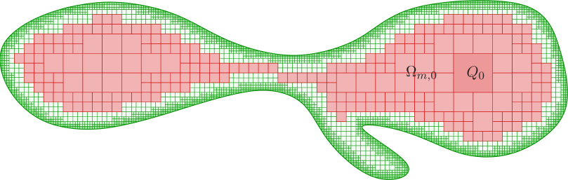
Figure 1. The set $\Omega_{m,\,0}$ is the path-component of the union of cubes of side-length at least $2^{-m}$ that contains $Q_{0}$. In order to have the properties listed in Lemma 2.4 for the subdomain $\Omega_{m}$ we will cut out those parts from $\Omega_{m,\,0}$ whose connection to $Q_{0}$ is blocked by dilated boundary cubes.

Define $\mathcal{W}_{m,\,0}$ to be the collection of the Whitney cubes in $\mathcal{W}$ that are contained in $\Omega_{m,\,0}$. Also let

$$\mathcal{D}_{m,\,0}=\left\{Q_{i}\in\mathcal{W}\colon Q_{i}\subset\Omega_{m,\,0},\,Q_{i}\cap\partial\Omega_{m,\,0}\neq\emptyset\right\}$$

and

$$D_{m,\,0}=\bigcup_{Q_{i}\in\mathcal{D}_{m,\,0}}Q_{i}.$$

Notice that, by definition, any Whitney cube $Q_{j}\in\mathcal{D}_{m,\,0}$ satisfies

$$2^{-m}\leq\ell(Q_{j})<2^{-m+2},$$ (2.1)

and thus there are at most finitely many of them since $\Omega$ is bounded. Up to relabeling all the $Q_{i}$’s in $\mathcal{W}$ we may assume that all the cubes in $\mathcal{D}_{m,\,0}$ are ordered consecutively from $1$ to some finite number $N_{0}$.

Recall the constant $C_{1}$ in Lemma 2.1. We next refine $\Omega_{m,\,0}$ according to the $C_{1}$-ball separation condition in order to obtain the desired set $\Omega_{m}$. It is constructed via an induction argument according to the cubes in $\mathcal{D}_{m,\,0}$.

First for each cube $Q_{j}\in\mathcal{D}_{m,\,0}$, we define $U_{j}=(5\sqrt{n}C_{1})_{\Omega}Q_{j}$. Let $m$ be large enough such that $U_{j}\cap Q_{0}=\emptyset$. For each $Q_{j}$ let $Block_{j}$ (which might be empty) be the union of all the path-components of $\Omega\setminus U_{j}$ not containing $Q_{0}$. Roughly speaking, the set $Block_{j}$ is the collection of points in $\Omega$ whose connection to $Q_{0}$ is blocked by $U_{j}$. As any curve joining $Q_{0}$ and some point outside $\Omega_{m,\,0}$ has to pass through $D_{m,\,0}$, the $C_{1}$-separation condition allows us to conclude that

$$\Omega=\Omega_{m,\,0}\cup\bigcup_{Q_{j}\in\mathcal{D}_{m,\,0}}U_{j}\cup\bigcup_{Q_{j}\in\mathcal{D}_{m,\,0}}Block_{j}.$$ (2.2)

Suppose that there exists $Q_{k}\in\mathcal{D}_{m}$ such that $U_{j}\cap U_{k}=\emptyset$ and $Block_{j}\cap U_{k}\neq\emptyset$. Then by the path-connectedness of $U_{k}\subset\Omega\setminus U_{j}$ and the definition of $Block_{j}$ we conclude that

$$U_{k}\subset Block_{j}.$$ (2.3)

Now let us define

$$\mathcal{W}_{m,\,1}=\left\{Q\in\mathcal{W}_{m,\,0}\colon Q\not\subset\left(Block_{1}\setminus(25\sqrt{n}C_{1})_{\Omega}Q_{1}\right)\right\}\subset\mathcal{W}_{m,\,0},$$

and

$$\Omega_{m,\,1}=\bigcup_{Q\in\mathcal{W}_{m,\,1}}Q\subset\Omega_{m,\,0}.$$

We also define

$$\mathcal{D}_{m,\,1}=\left\{Q_{i}\in\mathcal{D}_{m,\,0}\colon Q_{i}\subset\Omega_{m,\,1},\,Q_{i}\cap\partial\Omega_{m,\,1}\neq\emptyset\right\}.$$

We claim that

$$\Omega=\Omega_{m,\,1}\cup\bigcup_{Q_{j}\in\mathcal{D}_{m,\,1}}U_{j}\cup\bigcup_{Q_{j}\in\mathcal{D}_{m,\,1}}Block_{j}.$$ (2.4)

Indeed comparing to (2.2) we have three cases.

First of all if $y\in Block_{k}$ with $Q_{k}\notin\mathcal{D}_{m,\,1}$, then

$$Q_{k}\subset Block_{1}\setminus(25\sqrt{n}C_{1})_{\Omega}Q_{1}.$$

This with (2.1) gives us $U_{k}\cap U_{1}=\emptyset$, and consequently $U_{k}\subset Block_{1}$ by (2.3). Therefore any curve from $y$ to $Q_{0}$ needs to pass through $U_{1}$ by the definition of $Block_{1}$ and the $C_{1}$-ball-separation condition, and then by definition $y\in Block_{1}$.

Secondly if $y\in U_{k}$ with $Q_{k}\notin\mathcal{D}_{m,\,1}$, then again

$$Q_{k}\subset Block_{1}\setminus(25\sqrt{n}C_{1})_{\Omega}Q_{1}.$$

By the deduction above we similarly conclude that $y\in Block_{1}$.

At last suppose $y\in\Omega_{m,\,0}\setminus\Omega_{m,\,1}$. Then it belongs to some cube $Q$ originally in $\mathcal{W}_{m,\,0}$ but not in $\mathcal{W}_{m,\,1}$. Therefore

$$Q\subset Block_{1}\setminus(25\sqrt{n}C_{1})_{\Omega}Q_{1}.$$

However $Q$ is connected, and by the argument of (2.3) we also conclude that $y\in Block_{1}$. All in all we have shown (2.4).

If $Q_{2}\notin\mathcal{D}_{m,\,1}$, then we just let $\Omega_{m,\,2}=\Omega_{m,\,1}$ and accordingly define $\mathcal{D}_{m,\,2}$ and so on. Otherwise, we apply the procedure above, with $Q_{1}$ replaced by $Q_{2}$ and $Block_{1}$ replaced by $Block_{2}$, to obtain these sets (and collections). We repeat this process for every $Q_{j}$ with $3\leq j\leq N_{0}$. By iteration we finally obtain a set $\Omega_{m}:=\Omega_{m,\,N_{0}}$.

Notice that any Whitney cube in $\mathcal{W}_{m,\,N_{0}}$ intersecting $\partial\Omega_{m}$ is contained in $(60\sqrt{n}C_{1})_{\Omega}Q_{j}$ for some $1\leq j\leq N_{0}$. Thus it has edge length comparable to $2^{-m}$ with the constant only depending on $n$ and $C_{1}$. Hence there exists a constant $M=M(C_{1},\,n)$ such that

$$\Omega_{m}\subset\subset\Omega_{m^{\prime}}$$

whenever $m^{\prime}\geq m+M$. The deduction above together with the fact that $\Omega=\bigcup_{m}\Omega_{m,\,0}$ also gives

$$\Omega=\bigcup_{m}\Omega_{m}.$$

Moreover $\mathcal{D}_{m}:=\mathcal{D}_{m,\,N_{0}}$ consists of cubes from $\mathcal{D}_{m,\,0}$. To conclude, we obtain the following lemma.

Lemma 2.4.

Let $\Omega$ be a bounded domain which is $\delta$-Gromov hyperbolic with respect to the quasihyperbolic metric, $\mathcal{W}=\{Q_{j}\}$ be the collection of Whitney cubes of $\Omega$ and $Q_{0}$ be one of the largest Whitney cubes. Then there exists a sequence of sets $\Omega_{m}\subset\subset\Omega$ such that by setting

$$\mathcal{B}_{m}=\left\{Q_{j}\in\mathcal{W}\colon Q_{j}\subset\Omega_{m},\,Q_{j}\cap\partial\Omega_{m}\neq\emptyset\right\},$$

by letting $U_{j}=(5\sqrt{n}C_{1})_{\Omega}Q_{j}$ for each $Q_{j}\in\mathcal{B}_{m},$ and by finally defining $Block_{j}$ (which might be empty) to be the union of all the path-components of $\Omega\setminus U_{j}$ not containing $Q_{0}$, we have the following properties.

1. Each $\Omega_{m}$ consists of finitely many Whitney cubes and any two of them can be joined by a chain of Whitney cubes in $\Omega$ of edge lengths not less than $2^{-m}$. Moreover $Q_{0}\subset\Omega_{m}$ and there exists a constant $M=M(\delta,\,n)$ such that

   $$\Omega=\bigcup_{m}\Omega_{m},$$

   and

   $$\Omega_{m}\subset\subset\Omega_{m^{\prime}}$$

   for any $m^{\prime}\geq m+M$.

2. For every Whitney cube $Q_{j}\in\mathcal{B}_{m}$ we have $2^{-m}\leq\ell(Q_{j})\lesssim 2^{-m}$. We call such a cube a boundary cube of $\Omega_{m}$.

3. There exists a subcollection $\mathcal{D}_{m}$ of $\mathcal{B}_{m}$ such that for each $Q_{k}\in\mathcal{B}_{m}$ and $Q_{j}\in\mathcal{D}_{m}$

   $$Q_{k}\cap Block_{j}\neq\emptyset\ \Rightarrow\ Q_{k}\subset(60\sqrt{n}C_{1})_{\Omega}Q_{j}.$$

   Moreover $\{(60\sqrt{n}C_{1})_{\Omega}Q_{j}\}_{Q_{j}\in\mathcal{D}_{m}}$ covers all the boundary cubes of $\Omega_{m}$.

4. We have

   $$\Omega=\Omega_{m}\cup\bigcup_{Q_{j}\in\mathcal{D}_{m}}U_{j}\cup\bigcup_{Q_{j}\in\mathcal{D}_{m}}Block_{j}.$$

The property 3) above turns out to be crucial later and it may fail for $\mathcal{B}_{m}$; this is the reason for introducing the subcollection $\mathcal{D}_{m}$ of $\mathcal{B}_{m}$.

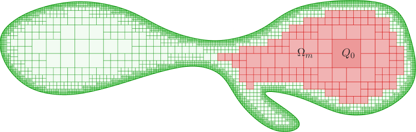
Figure 2. The set $\Omega_{m}$ obtained after the iterative procedure from sets $\Omega_{m,i}$ still contains the cube $Q_{0}$.

2.2. The decomposition of the boundary layer

In this subsection we first decompose $\Omega\setminus\Omega_{m}$ into two main parts $E_{m}$ and $F_{m}$, and then make further decompositions of them.

First of all let

$$E_{m}=\left(\bigcup_{Q_{j}\in\mathcal{D}_{m}}(70\sqrt{n}C_{1})_{\Omega}Q_{j}\right)\setminus\Omega_{m}.$$

Secondly, we denote by $F_{m}$ the rest of $\Omega$, that is,

$$F_{m}=\Omega\setminus(\Omega_{m}\cup E_{m}).$$

Notice that by Lemma 2.4 we have

$${\mathop{\mathrm{missing}}{\,dist\,}}_{\Omega}(F_{m},\,\Omega_{m})\geq 2^{-m},$$

and

$$F_{m}\subset\bigcup_{Q_{j}\in\mathcal{D}_{m}}Block_{j}$$

where the set $Block_{j}$ is defined in Lemma 2.4.

By abuse of notation, we also denote by $E_{m}$ and $F_{m}$ their closures with respect to the topology of $\Omega$, respectively. Observe that the boundary of $(c)_{\Omega}Q$ in $\Omega$ is porous and hence of Lebesgue measure zero,

$$|\partial(c)_{\Omega}Q\cap\Omega|=0,$$ (2.5)

for each $Q\in\mathcal{W}$ and each $c.$ Therefore we have

$$|\Omega_{m}\cap E_{m}|=|E_{m}\cap F_{m}|=0.$$

2.2.1. The decomposition of $E_{m}$

We decompose $E_{m}$ further. Recall that

$$E_{m}\subset\bigcup_{Q_{j}\in\mathcal{D}_{m}}(71\sqrt{n}C_{1})_{\Omega}Q_{j}.$$

Let $V_{j}=(71\sqrt{n}C_{1})_{\Omega}Q_{j}$ for each $Q_{j}\in\mathcal{D}_{m}$. For simplicity we again assume that

$$\mathcal{D}_{m}=\{Q_{1},\,\dots,\,Q_{N}\}$$

with some $N\leq N_{0}$. We claim that for each fixed $V_{j}$,

$$\#\left\{1\leq k\leq N\colon V_{j}\cap V_{k}\neq\emptyset\right\}\leq C(n,\,C_{1}),$$ (2.6)

where $\#$ means the cardinality of the corresponding set. Indeed, if $V_{j}\cap V_{k}\neq\emptyset$, then ${\mathop{\mathrm{missing}}{\,dist\,}}_{\Omega}(Q_{k},\,Q_{j})\lesssim 2^{-m}$ by the definition of $V_{j}$. Then (2.6) follows by the fact that $\ell(Q_{j})\sim 2^{-m}$ with a constant independent of $j$.

Define $S_{1}=V_{1}\cap E_{m}$, and inductively for $j\geq 2$ set

$$S_{j}=\left(V_{j}\setminus\bigcup_{i=1}^{j-1}V_{i}\right)\cap E_{m}.$$

Notice that $S_{j}$ may well be disconnected, or even empty. We replace every $S_{j}$ by its closure with respect to the topology of $\Omega$, and still use the notation $S_{j}$. Notice that after all these changes, $V_{j},\,S_{j}$ still satisfy all the corresponding properties above; especially

$$E_{m}\subset\bigcup_{j}S_{j}.$$

By (2.6) for each $S_{j}$

$$\#\left\{1\leq k\leq N\colon S_{j}\cap S_{k}\neq\emptyset\right\}\leq C(n,\,C_{1}),$$ (2.7)

and the corresponding $Q_{j},\,Q_{k}\in\mathcal{D}_{m}$ satisfy

$${\mathop{\mathrm{missing}}{\,dist\,}}_{\Omega}(Q_{j},\,Q_{k})\lesssim 2^{-m}.$$

Similar reasons also give the fact that

$$\#\left\{k\in\mathbb{N}\colon Q_{j}\in\mathcal{B}_{m},\,Q_{j}\cap S_{k}\neq\emptyset\right\}\leq C(n,\,C_{1}).$$ (2.8)

At last we remark that for any $j,\,k$

$$|S_{j}\cap S_{k}|=0$$

by (2.5). Moreover by the definition of $S_{j}$ we have

$${\mathop{\mathrm{missing}}{\,diam\,}}_{\Omega}(S_{j})\lesssim 2^{-m}.$$ (2.9)

2.2.2. The decomposition of $F_{m}$

Recall that $Q_{0}$ is one of the largest Whitney cubes contained in $\Omega_{m}$, and for each $Q_{j}\in\mathcal{D}_{m}$ we have $U_{j}=(5\sqrt{n}C_{1})_{\Omega}Q_{j}$ and $V_{j}=(71\sqrt{n}C_{1})_{\Omega}Q_{j}$.

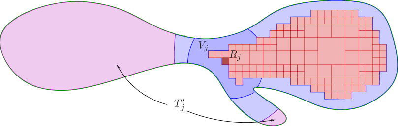
Figure 3. The set $T_{j}^{\prime}$ consist of all the path-components of $F_{m}$ for which the set $U_{j}$ centered at $Q_{j}$ blocks all curves going from the path-component to the cube $Q_{0}$.

To decompose the last part $F_{m}$, we introduce the following notation. Recall the definition of $Block_{j}$ in Lemma 2.4 and define

$$T^{\prime}_{j}=Block_{j}\cap F_{m}.$$

See Figure 3. Certainly $T^{\prime}_{j}$ could be empty. We replace $T^{\prime}_{j}$ by its closure with respect to the topology of $\Omega$ and still denote it by $T^{\prime}_{j}$. Notice that by Lemma 2.4

$$F_{m}=\bigcup_{j}T^{\prime}_{j}.$$

Fix $T^{\prime}_{j}$ and suppose that $T^{\prime}_{j}\cap S_{k}\neq\emptyset$. We claim that $V_{k}\cap V_{j}\neq\emptyset$. Indeed, if $V_{k}\cap V_{j}=\emptyset$, then $V_{k}\cap U_{j}=\emptyset$ and by the path-connectedness of $V_{k}$ any point $y\in T^{\prime}_{j}\cap V_{k}$ can be connected to $Q_{k}\in\mathcal{D}_{m}$ by a path in

$$V_{k}\subset\Omega\setminus U_{j}.$$

If $Q_{k}$ can be connected to $Q_{0}$ via a path in $\Omega\setminus U_{j}$, then $y$ can be connected to $Q_{0}$ via a path in $\Omega\setminus U_{j}$, which leads to a contradiction to the definition of $Block_{j}$, which contains $T^{\prime}_{j}$. Then our claim follows. If $Q_{k}$ cannot be connected to $Q_{0}$ via any path in $\Omega\setminus U_{j}$, then $Q_{k}\subset Block_{j}$, and by Lemma 2.4 we know that

$${\mathop{\mathrm{missing}}{\,dist\,}}_{\Omega}(Q_{k},\,Q_{j})\leq 60\sqrt{n}C_{1}{\mathop{\mathrm{missing}}{\,diam\,}}(Q_{j}).$$

The claim follows from the definition of $V_{j}$ .

Therefore by the proof of (2.6) and the definition of $S_{k}$ we conclude that, for each fixed (non-empty) $T^{\prime}_{j}$,

$$\#\left\{1\leq k\leq N\colon T^{\prime}_{j}\cap S_{k}\neq\emptyset\right\}\leq C(n,\,C_{1}).$$ (2.10)

Also note that if $y\in T^{\prime}_{j}\cap T^{\prime}_{k}$, then the path-component of $T^{\prime}_{j}$ containing $y$ is a subset of $T^{\prime}_{j}\cap T^{\prime}_{k}$ by the definition of $T^{\prime}_{j}$.

We define $T_{1}=T^{\prime}_{1}$, and for $j\geq 2$ set

$$T_{j}=T^{\prime}_{j}\setminus\bigcup_{i=1}^{j-1}T^{\prime}_{i}.$$

We also refer by $T_{j}$ to its closure with respect to the topology of $\Omega$.

According to (2.10) for each fixed non-empty $T_{j}$

$$\#\left\{1\leq k\leq N\colon T_{j}\cap S_{k}\neq\emptyset\right\}\leq C(n,\,C_{1}).$$ (2.11)

Similarly for each fixed $S_{j}$

$$\#\left\{1\leq k\leq N\colon S_{j}\cap T_{k}\neq\emptyset\right\}\leq C(n,\,C_{1}).$$ (2.12)

To conclude from the subsections above, whenever $Q_{j}\cap S_{k}\neq\emptyset$ with $Q_{j}\in\mathcal{B}_{m}$, $S_{j}\cap S_{k}\neq\emptyset$ or $T_{j}\cap S_{k}\neq\emptyset$ we always have the corresponding $Q_{j},\,Q_{k}\in\mathcal{B}_{m}$ satisfying

$${\mathop{\mathrm{missing}}{\,dist\,}}_{\Omega}(Q_{j},\,Q_{k})\lesssim 2^{-m}.$$

This fact with Lemma 2.4 allows us to apply Lemma 2.3 later.

2.3. A partition of unity

We construct a partition of unity in this subsection. To this end, let us introduce the following notation. For a set $A\subset\Omega$, we define

$$\mathcal{N}_{m,\,\Omega}(A)=\left\{x\in\Omega\colon{\mathop{\mathrm{missing}}{\,dist\,}}_{\Omega}(x,\,A)\leq 2^{-m-5}\right\}.$$

Lemma 2.5.

With all the notations above, there are functions $\psi$, $\phi_{j}$ and $\varphi_{j}$ with $1\leq j\leq N$ such that:

1. The function $\psi$ is Lipschitz in $\Omega$, compactly supported in $\Omega_{m}$, $0\leq\psi\leq 1$, and $|\nabla\psi(x)|\lesssim 2^{-m}$.

2. For each $j$, we have $\phi_{j}\in W^{1,\,\infty}(\Omega)$. The support of $\phi_{j}$ is relatively closed in $\Omega$ and contained in $\mathcal{N}_{m,\,\Omega}(S_{j})$, $0\leq\phi_{j}\leq 1$, and $|\nabla\phi_{j}|\lesssim 2^{m}$.

3. For each $j$, we have $\varphi_{j}\in W^{1,\,\infty}(\Omega)$. The support of $\varphi_{j}$ is relatively closed in $\Omega$ and contained in $\mathcal{N}_{m,\,\Omega}(T_{j})$, $0\leq\varphi_{j}\leq 1$, and $|\nabla\varphi_{j}|\lesssim 2^{m}$.

4. $\psi(x)+\sum_{j}\phi_{j}(x)+\sum_{j}\varphi_{j}(x)=1$ for any $x\in\Omega$.

Proof.

First of all we construct cut-off functions for each of our sets via the distance functions with respect to the inner metric. The function $\phi_{j}$ can be defined as

$$\phi_{j}(x)=\max\left\{1-2^{m+6}{\mathop{\mathrm{missing}}{\,dist\,}}_{\Omega}(x,\,S_{j}),\,0\right\},$$

and similarly

$$\varphi_{j}(x)=\max\left\{1-2^{m+6}{\mathop{\mathrm{missing}}{\,dist\,}}_{\Omega}(x,\,T_{j}),\,0\right\}.$$

The function $\psi$ is defined by

$$\psi(x)=\min\left\{2^{m+8}{\mathop{\mathrm{missing}}{\,dist\,}}_{\Omega}(x,\,E_{m}\cup F_{m}),\,1\right\}.$$

It is obvious that these functions satisfy

$$\psi(x)+\sum_{j}\phi_{j}(x)+\sum_{j}\varphi_{j}(x)\geq 1$$

for every $x\in\Omega$.

Note that by the essence of (2.8), (2.7), (2.11) and (2.12) we have for each $Q_{j}\in\mathcal{B}_{m}$

$$\#\left\{1\leq k\leq N\colon,\,Q_{j}\cap\mathcal{N}_{m,\,\Omega}(S_{k})\neq\emptyset\right\}\leq C(n,\,C_{1}),$$ (2.13)

and also for each $Q_{j}\in\mathcal{D}_{m}$

$$\#\left\{1\leq k\leq N\colon\mathcal{N}_{m,\,\Omega}(S_{j})\cap\mathcal{N}_{m,\,\Omega}(S_{k})\neq\emptyset\right\}\leq C(n,\,C_{1}),$$ (2.14)

$$\#\left\{1\leq k\leq N\colon\mathcal{N}_{m,\,\Omega}(S_{j})\cap\mathcal{N}_{m,\,\Omega}(T_{k})\neq\emptyset\right\}\leq C(n,\,C_{1}),$$ (2.15)

$$\#\left\{1\leq k\leq N\colon\mathcal{N}_{m,\,\Omega}(T_{j})\cap\mathcal{N}_{m,\,\Omega}(S_{k})\neq\emptyset\right\}\leq C(n,\,C_{1}).$$ (2.16)

Hence by the decomposition of $\Omega$ we conclude that for any $x\in\Omega$

$$\chi_{\Omega}(x)\leq\Phi(x):=\psi(x)+\sum_{j}\phi_{j}(x)+\sum_{j}\varphi_{j}(x)\lesssim\chi_{\Omega}(x).$$

Therefore, by dividing $\psi,\,\phi_{j},\,\varphi_{j}$ by $\Phi$, respectively, we obtain the desired partition of unity. The new functions, still denoted by $\psi,\,\phi_{j},\,\varphi_{j}$, satisfy the desired gradient control as $\Phi$ is bounded from below and above. ∎

Notice that

$$|\mathcal{N}_{m,\,\Omega}(S_{j})\setminus S_{j}|\lesssim 2^{-mn}$$ (2.17)

by (2.9) uniformly in $j.$ Moreover the proof of (2.10) also shows that there are uniformly finitely many $V_{k}$ such that $V_{k}$ intersects $N_{m,\,\Omega}(T_{j})\setminus T_{j}$. Thus

$$|\mathcal{N}_{m,\,\Omega}(T_{j})\setminus T_{j}|\lesssim 2^{-mn}.$$ (2.18)

Furthermore by an argument similar to the proof of (2.10), for every $1\leq j\leq N$ we conclude that

$$\#\left\{1\leq k\leq N\colon\mathcal{N}_{m,\,\Omega}(T_{j})\cap\mathcal{N}_{m,\,\Omega}(T_{k})\neq\emptyset\right\}\leq C(n,\,C_{1}).$$ (2.19)

3. Proof of Theorem 1.3

Proof of Theorem 1.3.

Fix $\epsilon>0$. Also fix $u\in W^{1,\,p}(\Omega)$ with $1\leq p<\infty$. We may assume that $u$ is smooth and bounded since bounded smooth functions are dense in $W^{1,\,p}(\Omega)$; e.g. see the proof of [11, Lemma 2.6]. We may further assume that $\|u\|_{L^{\infty}(\Omega)}=1$.

Recall that $\Omega=\Omega_{m}\cup E_{m}\cup F_{m}$. Define $D^{\prime}_{m}$ to be the union of those Whitney cubes $Q\in\mathcal{W}$ for which there exists a chain of no more than $M$ Whitney cubes joining $Q$ to some cube in $\mathcal{B}_{m}.$ Here the constant $M$ that depends on $C_{1},\,C_{2},\,n$ will be determined later. Then the quasihyperbolic distance from $Q$ to $\cup_{Q\in\mathcal{B}_{m}}Q$ is uniformly bounded if $Q\subset D^{\prime}_{m}.$ Observe that, for any Whitney cube $Q\subset D^{\prime}_{m}$ we have

$$\ell(Q)\lesssim 2^{-m},$$

with a constant depending on $C_{1},\,C_{2},\,n$. Also notice that Lemma 2.4 implies $|\Omega\setminus\Omega_{m}|\to 0$. Thus for $m\in\mathbb{N}$ large enough we have

$$\|u\|^{p}_{W^{1,\,p}(D^{\prime}_{m}\cup E_{m}\cup F_{m})}\leq\epsilon\ \text{ and }\ |E_{m}\cup F_{m}|\leq\epsilon.$$ (3.1)

Notice that $u|_{\Omega_{m}}\in W^{1,\,\infty}(\Omega_{m})$ since $\Omega_{m}$ is compact and $u$ is smooth. We define a function $u_{m}$ on $\Omega$ by setting

$$u_{m}(x)=u(x)\psi(x)+\sum_{j}a_{j}\phi_{j}(x)+\sum_{j}a_{j}\varphi_{j}(x),$$

where $\varphi(x)$, $\phi_{j}(x)$ and $\psi_{j}(x)$ are the functions in Lemma 2.5 and

$$a_{j}={\hbox to0.0pt{\bf\kern 4.49997pt--\hss}\int}\ignorespaces_{Q_{j}}u(x)\,dx$$

is the integral average over $Q_{j}\in\mathcal{B}_{m}$.

It is obvious that $u_{m}\in W^{1,\,\infty}(\Omega)$ by our construction, since by boundedness of $\Omega$ we only have finitely many $Q_{j}\in\mathcal{B}_{m}$ and Lemma 2.5 gives the estimates on the derivatives. Moreover we have $\|u_{m}\|_{L^{\infty}(\Omega)}\leq 1$ by our assumption, Lemma 2.5 and the definition of $u_{m}$. Hence $\|u_{m}\|_{L^{p}(\Omega\setminus\Omega_{m})}\leq\epsilon$ by (3.1). Consequently, by the definition of $\mathcal{N}_{m,\,\Omega}(\cdot)$ and Lemma 2.5, we only need to show that

$$\int_{(\Omega\setminus\Omega_{m})\cup(\bigcup_{Q\in\mathcal{B}_{m}}Q)}|\nabla u_{m}|^{p}\,dx\lesssim\epsilon.$$

We will show this via the Poincaré inequality, Lemma 2.3 and Lemma 2.5.

We write $G(Q_{j},\,Q_{k})$ for the union of the cubes given by Lemma 2.3 for each pair $Q_{j},\,Q_{k}\in\mathcal{B}_{m}$. Recall that ${\mathop{\mathrm{missing}}{\,dist\,}}_{\Omega}(F_{m},\,\Omega_{m})\geq 2^{-m}.$ Then for any $Q_{j}\in\mathcal{B}_{m}$ with the associated average $a_{j}$, by (2.13), (2.17), Lemma 2.3, Lemma 2.5 and the Poincaré inequality we obtain that

$$\int_{Q_{j}}|\nabla u_{m}|^{p}\,dx\lesssim\int_{Q_{j}}|\nabla(u_{m}-a_{j})|^{p}\,dx$$

$$\lesssim \int_{Q_{j}}|\nabla[(u(x)-a_{j})\psi(x)]|^{p}\,dx+\sum_{\begin{subarray}{c}S_{k}\subset E_{m}\\ Q_{j}\cap\mathcal{N}_{m,\,\Omega}(S_{k})\neq\emptyset\end{subarray}}\int_{Q_{j}}|\nabla[(a_{k}-a_{j})\phi_{k}(x)]|^{p}\,dx$$

$$\lesssim \int_{Q_{j}}|\nabla u|^{p}+|u(x)-a_{j}|^{p}2^{mp}\,dx+\sum_{\begin{subarray}{c}S_{k}\subset E_{m}\\ Q_{j}\cap\mathcal{N}_{m,\,\Omega}(S_{k})\neq\emptyset\end{subarray}}\int_{Q_{j}}|a_{k}-a_{j}|^{p}2^{mp}\,dx$$

$$\lesssim \int_{Q_{j}}|\nabla u|^{p}\,dx+\sum_{\begin{subarray}{c}S_{k}\subset E_{m}\\ Q_{j}\cap\mathcal{N}_{m,\,\Omega}(S_{k})\neq\emptyset\end{subarray}}2^{-m(n-p)}2^{-m(p-n)}\int_{G(Q_{j},\,Q_{k})}|\nabla u|^{p}\,dx$$

$$\lesssim \int_{Q_{j}}|\nabla u(x)|^{p}\,dx+\sum_{\begin{subarray}{c}S_{k}\subset E_{m}\\ Q_{j}\cap\mathcal{N}_{m,\,\Omega}(S_{k})\neq\emptyset\end{subarray}}\int_{G(Q_{j},\,Q_{k})}|\nabla u|^{p}\,dx.$$

Notice that by Lemma 2.3 there are uniformly finitely many cubes contained in the chain $G(Q_{j},\,Q_{k})$ connecting $Q_{j}$ and $Q_{k}$ if $\mathcal{N}_{m,\,\Omega}(S_{k})\cap Q_{j}\neq\emptyset$.

On the other hand recall that $\psi(x)$ is compactly supported in $\Omega_{m}$. Then for each $S_{j}$, Lemma 2.3, (2.9), (2.14), (2.15), (2.17) and the Poincaré inequality give

$$\int_{S_{j}}|\nabla u_{m}|^{p}\,dx\lesssim\int_{S_{j}}|\nabla(u_{m}-a_{j})|^{p}\,dx$$

$$\lesssim \sum_{\begin{subarray}{c}S_{k}\subset E_{m}\\ \mathcal{N}_{m,\,\Omega}(S_{j})\cap\mathcal{N}_{m,\,\Omega}(S_{k})\neq\emptyset\end{subarray}}\int_{S_{j}}|\nabla[(a_{k}-a_{j})\phi_{k}(x)]|^{p}\,dx$$

$$\qquad+\sum_{\begin{subarray}{c}T_{k}\subset F_{m}\\ \mathcal{N}_{m,\,\Omega}(S_{j})\cap\mathcal{N}_{m,\,\Omega}(T_{k})\neq\emptyset\end{subarray}}\int_{S_{j}}|\nabla[(a_{k}-a_{j})\varphi_{k}(x)]|^{p}\,dx$$

$$\lesssim \sum_{\begin{subarray}{c}S_{k}\subset E_{m}\\ \mathcal{N}_{m,\,\Omega}(S_{j})\cap\mathcal{N}_{m,\,\Omega}(S_{k})\neq\emptyset\end{subarray}}\int_{S_{j}}|a_{k}-a_{j}|^{p}2^{mp}\,dx+\sum_{\begin{subarray}{c}T_{k}\subset F_{m}\\ \mathcal{N}_{m,\,\Omega}(S_{j})\cap\mathcal{N}_{m,\,\Omega}(T_{k})\neq\emptyset\end{subarray}}\int_{S_{j}}|a_{k}-a_{j}|^{p}2^{mp}\,dx$$

$$\lesssim \sum_{\begin{subarray}{c}S_{k}\subset E_{m}\\ \mathcal{N}_{m,\,\Omega}(S_{j})\cap\mathcal{N}_{m,\,\Omega}(S_{k})\neq\emptyset\end{subarray}}2^{-m(p-n)}2^{-m(n-p)}\int_{G(Q_{j},\,Q_{k})}|\nabla u|^{p}\,dx$$

$$\qquad+\sum_{\begin{subarray}{c}T_{k}\subset F_{m}\\ \mathcal{N}_{m,\,\Omega}(S_{j})\cap\mathcal{N}_{m,\,\Omega}(T_{k})\neq\emptyset\end{subarray}}2^{-m(p-n)}2^{-m(n-p)}\int_{G(Q_{j},\,Q_{k})}|\nabla u|^{p}\,dx$$

$$\lesssim \sum_{\begin{subarray}{c}S_{k}\subset E_{m}\\ \mathcal{N}_{m,\,\Omega}(S_{j})\cap\mathcal{N}_{m,\,\Omega}(S_{k})\neq\emptyset\end{subarray}}\int_{G(R_{j},\,R_{k})}|\nabla u|^{p}\,dx+\sum_{\begin{subarray}{c}T_{k}\subset F_{m}\\ N_{m,\,\Omega}(S_{j})\cap\mathcal{N}_{m,\,\Omega}(T_{k})\neq\emptyset\end{subarray}}\int_{G(Q_{j},\,Q_{k})}|\nabla u|^{p}\,dx.$$

The calculation for $T_{j}$ is almost the same. Indeed by (2.16), (2.18), (2.19) and the Poincaré inequality

$$\int_{T_{j}}|\nabla u_{m}|^{p}\,dx\lesssim\int_{T_{j}}|\nabla(u_{m}-a_{j})|^{p}\,dx$$

$$\lesssim \sum_{\begin{subarray}{c}S_{k}\subset E_{m}\\ \mathcal{N}_{m,\,\Omega}(T_{j})\cap\mathcal{N}_{m,\,\Omega}(S_{k})\neq\emptyset\end{subarray}}\int_{T_{j}}|\nabla[(a_{k}-a_{j})\phi_{i}(x)]|^{p}\,dx$$

$$\qquad+\sum_{\begin{subarray}{c}T_{k}\subset F_{m}\\ \mathcal{N}_{m,\,\Omega}(T_{j})\cap\mathcal{N}_{m,\,\Omega}(T_{k})\neq\emptyset\end{subarray}}\int_{T_{j}}|\nabla[(a_{k}-a_{j})\phi_{i}(x)]|^{p}\,dx$$

$$\lesssim \sum_{\begin{subarray}{c}S_{k}\subset E_{m}\\ \mathcal{N}_{m,\,\Omega}(T_{j})\cap\mathcal{N}_{m,\,\Omega}(S_{k})\neq\emptyset\end{subarray}}\int_{T_{j}}|a_{k}-a_{j}|^{p}2^{mp}\,dx+\sum_{\begin{subarray}{c}T_{k}\subset F_{m}\\ \mathcal{N}_{m,\,\Omega}(T_{j})\cap\mathcal{N}_{m,\,\Omega}(T_{k})\neq\emptyset\end{subarray}}\int_{T_{j}}|a_{k}-a_{j}|^{p}2^{mp}\,dx$$

$$\lesssim \sum_{\begin{subarray}{c}S_{k}\subset E_{m}\\ \mathcal{N}_{m,\,\Omega}(T_{j})\cap\mathcal{N}_{m,\,\Omega}(S_{k})\neq\emptyset\end{subarray}}2^{-m(p-n)}2^{-m(n-p)}\int_{G(Q_{j},\,Q_{j})}|\nabla u|^{p}\,dx$$

$$\qquad+\sum_{\begin{subarray}{c}T_{k}\subset F_{m}\\ \mathcal{N}_{m,\,\Omega}(T_{j})\cap\mathcal{N}_{m,\,\Omega}(T_{k})\neq\emptyset\end{subarray}}2^{-m(p-n)}2^{-m(n-p)}\int_{G(Q_{j},\,Q_{j})}|\nabla u|^{p}\,dx$$

$$\lesssim \sum_{\begin{subarray}{c}S_{k}\subset E_{m}\\ \mathcal{N}_{m,\,\Omega}(T_{j})\cap\mathcal{N}_{m,\,\Omega}(S_{k})\neq\emptyset\end{subarray}}\int_{G(Q_{j},\,Q_{k})}|\nabla u|^{p}\,dx+\sum_{\begin{subarray}{c}T_{k}\subset F_{m}\\ \mathcal{N}_{m,\,\Omega}(T_{j})\cap\mathcal{N}_{m,\,\Omega}(T_{k})\neq\emptyset\end{subarray}}\int_{G(Q_{j},\,Q_{k})}|\nabla u|^{p}\,dx.$$

By Lemma 2.3, there is a constant $C_{3}=C_{3}(C_{1},\,C_{2},\,n)$ such that, for any chain of cubes $G(Q_{j},\,Q_{k})$ used above the number of cubes involved is uniformly bounded from above by $C_{3}$. This gives us the constant $M$ in the definition of $D^{\prime}_{m}$.

Sum over all the $Q_{j}$’s, $S_{j}$’s and $T_{j}$’s above. Notice that, since the number of Whitney cubes in any chain $G(Q_{j},\,Q_{k})$ above is always uniformly bounded by Lemma 2.3, the Whitney cubes involved in our sums have uniformly finite overlaps. Additionally all the cubes in these chains are contained in $D^{\prime}_{m}$. Thus we obtain (3.1) and conclude the first part of the theorem.

When $\Omega$ is quasiconvex, we immediately have that $C^{\infty}(\mathbb{R}^{n})$ is dense in $W^{1,\,p}(\Omega)$ since every function in $W^{1,\,\infty}(\Omega)$ can then be extended to a global Lipschitz function; by applying suitable cut-off functions and via a diagonal argument we obtain the approximation by smooth functions.

The argument for the Jordan domain case is similar to the proof of [11, Corollary 1.2]. Recall that for any two non-empty subsets $X$ and $Y$ of $\mathbb{R}^{n}$, the Hausdorff distance ${\mathop{\mathrm{missing}}{\,dist\,}}_{\mathrm{H}}(X,\,Y)$ is defined as

$${\mathop{\mathrm{missing}}{\,dist\,}}_{\mathrm{H}}(X,\,Y)=\max\{\,\sup_{x\in X}\inf_{y\in Y}d(x,\,y),\,\sup_{y\in Y}\inf_{x\in X}d(x,\,y)\}.$$

When $\Omega$ is Jordan, we can construct a sequence of Lipschitz domains $\{G_{s}\}_{s=1}^{\infty}$ approaching $\Omega$ in Hausdorff distance such that $\Omega\subset\subset G_{s+1}\subset\subset G_{s}$ and

$${\mathop{\mathrm{missing}}{\,dist\,}}_{\mathrm{H}}(G_{s},\,\partial\Omega)\leq 2^{-s}$$

for each $s\in\mathbb{N}$. For example, by the Morse-Sard theorem we may define $G_{s}$ via the boundary of a suitable lower level set of $d$, where $d$ is a smooth function obtained by applying suitable mollifiers and a partition of unity for $\mathbb{R}^{n}\setminus\Omega$ to the distance function ${\mathop{\mathrm{missing}}{\,dist\,}}(x,\,\Omega)$.

Now fix $m\in\mathbb{N}$ and choose $s$ such that $s\geq 2m$. Then, by the definition of $G_{s},$ the $2C_{1}$-separation condition with respect to $G_{s}$ holds for our original cubes in $\Omega_{m}$. Similarly for points with inner distance smaller than a multiple of $2^{-m}$ in $\Omega_{m}$, the $2C_{2}$-Gehring-Hayman condition with respect to $G_{s}$ still holds. Moreover, the original Whitney cubes contained in $\Omega_{m}$ are also Whitney-type for $G_{s}$ up to a multiplicative constant $2$ in Lemma 2.2. Therefore we may repeat all the arguments above similarly to extend the function $u_{m}$ from $\Omega_{m}$ to $v_{m}\in W^{1,\,p}(G_{s})$, with

$$\|u-v_{m}\|_{W^{1,\,p}(\Omega)}\lesssim\epsilon.$$

Since each $G_{s}$ is a Lipschitz domain, we may extend $v_{m}$ to a global Sobolev function, and then by applying suitable mollifiers and via a diagonal argument we obtain the approximation by global smooth functions. ∎

4. Proof of Theorem 1.1

When $n\geq 3$, unlike in the planar case, simply connectivity does not guarantee that $W^{1,\,\infty}(\Omega)$ be dense in $W^{1,\,p}(\Omega)$ for $1\leq p<\infty$. Indeed, given $1<p<\infty$ there exists a simply connected bounded domain $\Omega\subset\mathbb{R}^{3}$ such that even $W^{1,\,p}(\Omega)$ is not dense in $W^{1,\,q}(\Omega)$ for $1\leq q<p$.

Towards this, let us recall the definition of removable sets. A closed set $E\subset\mathbb{R}^{n}$ with Lebesgue measure zero is said to be removable for $W^{1,\,p}$ if

$$W^{1,\,p}(\mathbb{R}^{n})=W^{1,\,p}(\mathbb{R}^{n}\setminus E)$$

in the sense of sets. In [10, Theorem A], for any $1<p\leq n$, Koskela gave an example of a compact set $E\subset\mathbb{R}^{n}$ which is removable for $W^{1,\,p}$ but not for $W^{1,\,q}$ with $1\leq q<p$. We give a related planar example for every $1<p<\infty$.

Theorem 4.1.

Let $1<p<\infty$. Then there is a compact set $E\subset\mathbb{R}^{2}$ of Lebesgue measure zero such that $E$ is removable for $W^{1,\,q}$ when $p<q<\infty$ but not for $W^{1,\,q}$ when $1\leq q\leq p$.

By taking the union of a suitable collection of scaled and translated copies $E_{i}$ of the above compact sets corresponding to an increasing sequence of $p_{i}$ tending to a fixed $p$ we obtain the following corollary.

Corollary 4.2.

Let $1<p<\infty.$ Then there is a compact set $E\subset\mathbb{R}^{2}$ of Lebesgue measure zero such that $E$ is removable for $W^{1,\,q}$ when $q\geq p$ but not for $W^{1,\,q}$ when $1\leq q<p.$

We divide the proof of Theorem 4.1 into two lemmas.

Lemma 4.3.

Let $1<p\leq 2$. Then there is a compact set $E\subset\mathbb{R}^{2}$ of Lebesgue measure zero such that $E$ is removable for $W^{1,\,q}$ when $p<q<\infty$ but not for $W^{1,\,q}$ when $1\leq q\leq p$.

Proof.

The proof essentially follows from the proof of [10, Theorem A].

We first consider the case where $1<p<2$. By [10, Proposition 2.1, Theorem 2.2, Theorem 2.3] it suffices to construct a Cantor set $E\subset[0,\,1]$ of positive length so that, by letting $I_{j}$ be the complementary intervals of $E$ on $[0,\,1]$ and $\mathscr{H}^{1}$ the $1$-dimensional Hausdorff measure,

$$\sum_{j=1}^{\infty}\mathscr{H}^{1}(I_{j})^{2-p}<\infty,$$

while $E$ is $q$-porous for all $p<q\leq 2$. Recall that $E\subset[0,\,1]$ is $q$-porous if for $\mathscr{H}^{1}$-almost every point $x\in E$ there is a sequence of numbers $r_{i}$ and a constant $C_{x}$ such that $r_{i}\to 0$ as $i\to\infty$, and each interval $[x-r_{i},\,x+r_{i}]$ contains an interval $I_{i}\subset[0,\,1]\setminus E$ with $\mathscr{H}^{1}(I_{i})\geq C_{x}r_{i}^{\frac{1}{2-q}}$.

Towards this construction, we let $0<s<\frac{1}{3}$ be a small constant to be determined momentarily. Out set $E$ is obtained via the following Cantor construction. At the $i$-th step with $i\in\mathbb{N}$ we delete an open interval of length $si^{-\frac{2}{2-p}}2^{-\frac{i+1}{2-p}}$ from the middle of each of the remaining $2^{i}$ closed intervals with equal length, respectively. Then E is defined as the intersection of all these closed intervals, and $s$ is chosen such that

$$\sum_{i}s2^{i}i^{-\frac{2}{2-p}}2^{-\frac{i+1}{2-p}}<1.$$

Thus $E$ has positive length, and it is not difficult to check that $E$ has the desired properties.

When $p=2$ we similarly construct $E$ by removing intervals of length $s2^{-i}\exp(-2^{i})$ with sufficiently small (and fixed) $s$ at $i$-th step. Then by the proof of [10, Theorem A] and [10, Theorem 3.1], $E$ is not $q$-removable for any $1<q\leq 2$. The removability of $E$ for $q>2$ comes from [10, Proposition 2.1] again. ∎

Lemma 4.4.

Let $2<p<\infty$. Then there is a compact set $E\subset\mathbb{R}^{2}$ of Lebesgue measure zero such that $E$ is removable for $W^{1,\,q}$ when $p<q<\infty$ but not for $W^{1,\,q}$ when $1\leq q\leq p$.

Proof.

We separate our proof into three steps.

Step 1: The construction of $E$. The set $E$ is defined as a product set $C\times F$, where $C\subset\mathbb{R}$ is a Cantor set of Hausdorff dimension less than $1$ and $F\subset\mathbb{R}$ is a Cantor set with positive Lebesgue measure, called a fat Cantor set.

Let us start with the construction of $C$. Given a sequence $\{\lambda_{i}\}_{i\in\mathbb{N}_{+}}$ with $0<\lambda_{i}<\frac{1}{2}$, we build a symmetric Cantor set with $\lambda_{i}$ as the contraction ratio at step $i$. More precisely, define

$$C=\bigcap_{i=0}^{\infty}C_{i},$$

where $C_{0}=I_{0,1}=[0,1]$ and $C_{i}$ with $i\geq 1$ are defined iteratively as follows: When $I_{i,j}=[a,b]$ has been defined, let $I_{i+1,2j-1}=[a,a+\lambda_{i}|a-b|]$ and $I_{i+1,2j}=[b-\lambda_{i}|a-b|,b]$. This is well-defined as $\lambda_{i}<\frac{1}{2}$. Then we set

$$C_{i}=\bigcup_{j=1}^{2^{i}}I_{i,j}.$$

For the fat Cantor set $F$, likewise we associate it with a sequence of positive real numbers $(\beta_{i})_{i=1}^{\infty}$ such that

$$\beta_{i}=(1-\lambda_{i+1})P_{i}$$

where $P_{i}=\lambda_{1}\lambda_{2}\cdots\lambda_{i}$, and $\lambda_{i}$ are from the previous paragraph. Clearly

$$\sum_{i=1}^{\infty}\beta_{i}<1$$ (4.1)

as $\lambda_{i}<1$. The numbers $\beta_{i}$ denote the lengths of the disjoint open intervals removed from the unit interval. To be more specific, we define the approximating sequence $F_{i}\subset\mathbb{R}$ with respect to $\beta_{i}$ in the following way. Let $F_{0}=[0,1]$. Then iteratively, at step $n$, we replace one of the largest remaining intervals $[a,b]$ of the set $F_{n-1}$ by the set

$$\left[a,a+r\right]\cup\left[a+r+\beta_{n},b\right],\quad\text{where}\quad r=\frac{1}{2}\left(b-a-\sum_{i=n}^{\infty}\beta_{i}\right)$$ (4.2)

and obtain $F_{n}$ in this way. We claim that, there is always one interval in $F_{n}$ that has length strictly larger than $\sum_{i=n+1}^{\infty}\beta_{i}$. If so, then $F$ is well-defined.

Indeed when $n=0$ our claim follows immediately (4.1). Then under the induction assumption that there is an interval $[a,\,b]\subset F_{n-1}$ satisfying $b-a>\sum_{i=n}^{\infty}\beta_{i}$, we further have that at the $n$-th step by (4.2) there is an interval with length

$$b-a-r-\beta_{n}=\frac{1}{2}\left(b-a-\beta_{n}+\sum_{i=n+1}^{\infty}\beta_{i}\right)>\sum_{i=n+1}^{\infty}\beta_{i},$$

where the last inequality comes from the induction assumption. Therefore the largest interval in $F_{n}$ has length strictly larger than $\sum_{i=n+1}^{\infty}\beta_{i}$. Thus our claim follows. Moreover the length of the largest remaining interval in $F_{n}$ goes to zero as $n\to\infty$ by (4.2). Thus $F$ is a topological Cantor set. The fact that $\mathscr{H}^{1}(F)>0$ comes from (4.1).

Step 2: The unremovability of $E$ for $q\leq p$. Fix $p>2$ and a set $E=C\times F$ from the Step 1, with the sequence $\{\lambda_{i}\}$ to be determined later. Let $1\leq q\leq p$. We define a function $v\in W^{1,\,q}(\mathbb{R}^{2}\setminus E)$ such that it cannot be extended to $W^{1,\,q}(\mathbb{R}^{2})$. To do this, we first construct a function $u\in L^{\infty}(\mathbb{R}^{2}\setminus E)$ with $\nabla u\in L^{q}(\mathbb{R}^{2}\setminus E)$.

Let $u(x,\,y)=0$ if $x<0$ and $u(x,\,y)=1$ if $x>1$. For each $y\in F$ further define

$$u(x,\,y)=\frac{2j-1}{2^{i+1}}\quad\text{ for $\ x\in I_{i,\,j}\setminus(I_{i+1,\,2j-1}\cup I_{i+1,\,2j})$},$$

where $i\in\mathbb{N},\,1\leq j\leq 2^{i}.$ Then for $y\in F$, $u(x,\,y)$ is a Cantor step function with respect to $x$ if we extend it continuously. In Figure 4 we give an example of such a function.

Next we define $u(x,\,y)$ for $y\not\in F$. For $(x,\,y)\in[0,\,1]^{2}\setminus E$ and ${\mathop{\mathrm{missing}}{\,dist\,}}(y,\,F)\leq{\mathop{\mathrm{missing}}{\,dist\,}}(x,\,C)$ we also set

$$u(x,\,y)=\frac{2j-1}{2^{i+1}}\quad\text{ for $\ x\in I_{i,\,j}\setminus(I_{i+1,\,2j-1}\cup I_{i+1,\,2j})$},$$

where $i\in\mathbb{N},\,1\leq j\leq 2^{i}.$ Then for fixed $y_{0}\notin F$, on the horizontal line $y=y_{0}$ we have already defined the function $u$ up to finitely many open intervals. We then simply define $u$ as an affine function on each remaining interval so that it is continuous on this line. Then $u$ is defined in $\mathbb{R}^{2}\setminus E$, and the set

$$\left\{(x,\,y)\colon u(x,\,y)=\frac{2j-1}{2^{i+1}}\right\}$$

has Lipschitz boundary.

We claim that $u$ is also continuous in $\mathbb{R}^{2}\setminus E$. Indeed if ${\mathop{\mathrm{missing}}{\,dist\,}}(y,\,F)<{\mathop{\mathrm{missing}}{\,dist\,}}(x,\,C)$, then by definition $u$ is locally constant and hence certainly continuous. For the remaining case where $0\neq{\mathop{\mathrm{missing}}{\,dist\,}}(y,\,F)\geq{\mathop{\mathrm{missing}}{\,dist\,}}(x,\,C)$, there is an open interval $I$ such that $y\in I$, $I\cap F=\emptyset$, and for every $y_{0}\in I$ the function $u(x,\,y_{0})$ is Lipschitz with the constant depending only on ${\mathop{\mathrm{missing}}{\,dist\,}}(y_{0},\,F)$ (as $E$ is already fixed). Then for any such an $x$, in the vertical direction $u$ is also continuous since the affine-extension is done with respect to domains where $u$ is locally constant and whose boundary is a $1$-Lipschitz graph. Consequently, $u$ is even locally Lipschitz. Hence $u$ is a continuous function.

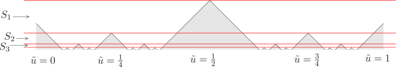
Figure 4. An illustration of the definition of $u$ for $\lambda_{i}=\frac{1}{3}$. On the $x$-axis the function $u$ is defined as the Cantor step function. The constant regions are extended to the complement as shown by the gray areas. For any horizontal line there are finitely many open intervals where the function is not defined by the previous extension. On each such interval we extend it as an affine function. We then estimate $|\nabla u|$ separately on each horizontal strip $S_{i}$.

We next estimate the Sobolev-norm of $u$. First up to a suitable translation we consider $u$ in a strip $S_{i}$ which is defined as

$$S_{i}=\mathbb{R}\times\left[\frac{1}{2}(1-\lambda_{i+1})P_{i},\frac{1}{2}(1-\lambda_{i})P_{i-1}\right],$$

and is a part of $\mathbb{R}^{2}\setminus E$ (up to a suitable translation). Also recall that $P_{i}=\lambda_{1}\lambda_{2}\cdots\lambda_{i}.$ Then each $S_{i}$ minus the triangles where the function is defined as constant has at most $2^{i}$ connected components $K$.

Up to another translation, each component $K$ equals

$$\left\{(x,y)\in\mathbb{R}^{2}\colon|x|<y,\,\frac{1}{2}(1-\lambda_{i+1})P_{i}<y<\frac{1}{2}(1-\lambda_{i})P_{i-1}\right\}$$

and up to adding a constant the function $u$ restricted on it is defined as

$$\tilde{u}(x,y)=2^{-i-1}\frac{x}{y};$$

see Figure 5. Thus $|\nabla\tilde{u}|\lesssim 2^{-i}P_{i}^{-1}$ in the strip $S_{i}$. Since each of the $2^{i}$ components $K$ have width and height comparable to $P_{i}$, we get

$$\int_{S_{i}}|\nabla\tilde{u}|^{q}\lesssim 2^{i}P_{i}^{2}\left(2^{-i}P_{i}^{-1}\right)^{q}=2^{i(1-q)}P_{i}^{2-q}.$$

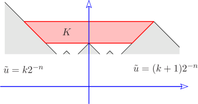
Figure 5. Each strip $S_{i}$ consists of $2^{i}$ connected components outside the regions where $\tilde{u}$ was initially defined as constant. Such a component $K$ is drawn here in the case $\lambda_{i}=\frac{1}{3}$. Also the choice of the coordinates used in the estimate is indicated in the figure.

Let us recall that $\beta_{i}=(1-\lambda_{i+1})P_{i}$. This implies that we only have copies of $S_{i}$ in $\mathbb{R}\times(F_{j-1}\setminus F_{j})$ with $i\geq j$. Consequently we have

$$\int_{\mathbb{R}^{2}\setminus E}|\nabla u|^{q}\lesssim\sum_{j=1}^{\infty}\sum_{i=j}^{\infty}2\int_{S_{i}}|\nabla\tilde{u}|^{q}\lesssim\sum_{i=1}^{\infty}2i\int_{S_{i}}|\nabla\tilde{u}|^{q}\lesssim\sum_{i=1}^{\infty}i2^{i(1-q)}P_{i}^{2-q}.$$ (4.3)

By Hölder’s inequality and the fact that $E$ is compact, it suffices to check the non-removability for the case $q=p$.

Choose $\lambda_{i}$ in such a way that

$$2^{i(1-p)}P_{i}^{2-p}=\frac{1}{i^{3}}$$ (4.4)

for all $i$ large enough. That is,

$$\lambda_{i}=\min\left\{\frac{1}{3},\,\frac{P_{i}}{P_{i-1}}\left(\frac{(i-1)^{3}2^{(i-1)(1-p)}}{i^{3}2^{i(1-p)}}\right)^{\frac{1}{2-p}}\right\}=\min\left\{\frac{1}{3},\,2^{\frac{p-1}{2-p}}\left(\frac{i}{i-1}\right)^{\frac{3}{p-2}}\right\}.$$

Observe that $\lambda_{i}\sim 2^{\frac{p-1}{2-p}}$ with the constant independent of $i$. With this choice

$$\sum_{i=1}^{\infty}i2^{i(1-p)}P_{i}^{2-p}=\sum_{i=1}^{\infty}\frac{1}{i^{2}}<\infty.$$

Therefore by (4.3) we conclude that $\nabla u\in L^{p}(\mathbb{R})$.

By letting

$$v=u\varphi,$$

where $\varphi\in C^{\infty}_{c}(\mathbb{R}^{2})$ has support in $[-1,\,2]^{2}$ and satisfies $\varphi(x)=1$ for $x\in[0,\,1]^{2}$, we have $v\in W^{1,\,p}(\mathbb{R}^{2}\setminus E)$. However $v$ cannot be extended to a function in $W^{1,\,p}(\mathbb{R}^{2}).$ Indeed, by the Sobolev embedding theorem for $p>2,$ the precise representative of an extension $w\in W^{1,\,p}(\mathbb{R}^{2})$ would continuous, while by definition the extension of $v$ is a Cantor function (multiplied by a smooth function) when restricted to $y=y_{0}$ for $y_{0}\in F$ with $|F|>0$. This would contradict the fact that the precise representative of a Sobolev function is absolutely continuous along almost every line parallel to the coordinate axes; see [6, 4.5.3, 4.9.2].

Step 3: The removability of $E$ for $q>p$. We claim that, for the set $E$ defined above, for every two points $z_{1},\,z_{2}\in\mathbb{R}^{2}\setminus E$ there is a curve $\gamma\subset\mathbb{R}^{2}\setminus E$ such that

$$\int_{\gamma}{\mathop{\mathrm{missing}}{\,dist\,}}(z,\,E)^{\frac{1}{1-q}}\,ds(z)\leq C(p,\,q)|z_{1}-z_{2}|^{\frac{q-2}{q-1}}.$$ (4.5)

If so, then by [13, Theorem 1.1] (or by [9]), we conclude that any function in $W^{1,\,q}(\mathbb{R}^{2}\setminus E)$ can be extended to $W^{1,\,q}(\mathbb{R}^{2})$. Since the Lebesgue measure of $E$ is zero, it follows that $W^{1,\,q}(\mathbb{R}^{2}\setminus E)=W^{1,\,q}(\mathbb{R}^{2})$ and hence $E$ is removable for $W^{1,\,q}(\mathbb{R}^{2})$.

Now let us show the claim. We only consider the case where $z_{1},\,z_{2}\in[0,\,1]^{2}$, as the general case can be easily reduced to it. For any $z_{1},\,z_{2}\in[0,\,1]^{2}\setminus E$, we write $z_{1}=(x_{1},\,y_{1})$ and $z_{2}=(x_{2},\,y_{2})$. First we may assume that $y_{1},\,y_{2}\notin F$. Indeed if $y_{1}\in F$ then $x_{1}\notin C$. Then there is a removed interval $I\subset[0,\,1]$ (in the construction of $C$) containing $x_{1}$. Find a point $x\in I$ such that

$$3|x-x_{1}|\leq\min\{|z_{1}-z_{2}|,\,{\mathop{\mathrm{missing}}{\,diam\,}}(I)\}\ \text{ and }\ 3{\mathop{\mathrm{missing}}{\,dist\,}}(x,\,C)\geq\min\{|z_{1}-z_{2}|,\,{\mathop{\mathrm{missing}}{\,diam\,}}(I)\};$$

the existence of such an $x$ follows from the triangle inequality. Let $w_{1}=(x,\,y_{1})$. Next since $F$ is topologically a Cantor set, as $y_{1}\in F$ one can find a point $z_{1}^{\prime}=(x,\,y_{1}^{\prime})$ such that $3|y_{1}-y_{1}^{\prime}|\leq|z_{1}-z_{2}|$ and $y_{1}^{\prime}\notin F$. Then the curve consisting of the two line segments $[z_{1},\,w_{1}]$ and $[w_{1},\,z_{1}^{\prime}]$ satisfies

$$\int_{[z_{1},\,w_{1}]\cup[w_{1},\,z_{1}^{\prime}]}{\mathop{\mathrm{missing}}{\,dist\,}}(z,\,E)^{\frac{1}{1-q}}\,ds(z)\lesssim\int_{0}^{|z_{1}-z_{2}|}t^{\frac{1}{1-q}}\,dt+|z_{1}-z_{2}|^{\frac{2-q}{1-q}}\lesssim|z_{1}-z_{2}|^{\frac{q-2}{q-1}},$$

with the constant depending only on $q$. We may also apply a similar argument for $z_{2}$. Thus our assumption is legitimate.

Under such an assumption we are going to construct the curve connecting $z_{1},\,z_{2}$. Recall that $\lambda_{i}\sim 2^{\frac{p-1}{2-p}}$ and $P_{i}=\lambda_{1}\lambda_{2}\cdots\lambda_{i}$. Then there is a natural number $n$ such that $P_{n+1}\leq|z_{1}-z_{2}|\leq P_{n}$. Notice that there is an interval $I_{0}\in\{I_{n,\,k}\}_{k=1}^{2^{n}}$ such that

$$\max\{{\mathop{\mathrm{missing}}{\,dist\,}}(I_{0},\,z_{1}),\,{\mathop{\mathrm{missing}}{\,dist\,}}(I_{0},\,z_{2})\}\lesssim|z_{1}-z_{2}|\ \text{ and }\ {\mathop{\mathrm{missing}}{\,diam\,}}(I_{0})=P_{n}$$

with the constant depend only on $p$ by the Cantor construction. Denote by $x_{0}$ the middle point of such an interval. Let $\gamma=[z_{1},\,(x_{0},\,y_{1})]\cup[(x_{0},\,y_{1}),\,(x_{0},\,y_{2})]\cup[(x_{0},\,y_{2}),\,z_{2}]$ be the curve joining $z_{1},\,z_{2}$ and consisting of three line segments; see Figure 6. We show that $\gamma$ is the desired curve.

Figure 6. We connect any two points $z_{1},z_{2}\in\mathbb{R}^{2}\setminus E$ (up to a negligible error near the end-points) with a curve consisting of a vertical part $\gamma_{\text{vert}}=[(x_{0},\,y_{1}),\,(x_{0},\,y_{2})]$ and two horizontal parts $\gamma_{\text{hor}}^{1}=[z_{1},\,(x_{0},\,y_{1})]$, $\gamma_{\text{hor}}^{2}=[(x_{0},\,y_{2}),\,z_{2}]$. The desired estimate on the vertical part comes from the almost self-similarity of the Cantor set $C$ with dimension strictly less than $1$, whereas for the horizontal parts we have to make a bit more careful estimate.

In fact for the vertical part $[(x_{0},\,y_{1}),\,(x_{0},\,y_{2})]$, as $x_{0}$ is the middle point of $I_{0}$ with ${\mathop{\mathrm{missing}}{\,diam\,}}(I_{0})=P_{n}$ and $\lambda_{i}\sim 2^{\frac{p-1}{2-p}}$, we have

$$\int_{[(x_{0},\,y_{1}),\,(x_{0},\,y_{2})]}{\mathop{\mathrm{missing}}{\,dist\,}}(z,\,E)^{\frac{1}{1-q}}\,ds(z)\lesssim|z_{1}-z_{2}|^{\frac{q-2}{q-1}},$$

with the constant depending only on $p$ and $q$. Hence it suffices for us to consider the horizontal ones.

First of all

$$\int_{[z_{1},\,(x_{0},\,y_{1})]}{\mathop{\mathrm{missing}}{\,dist\,}}(z,E)^{\frac{1}{1-q}}\,ds(z) \lesssim\sum_{i=n}^{\infty}2^{i-n}\int_{0}^{P_{i}}t^{\frac{1}{1-q}}\ dt\lesssim\sum_{i=n}^{\infty}2^{i-n}P_{i}^{\frac{q-2}{q-1}}$$

$$\lesssim|z_{1}-z_{2}|^{\frac{q-2}{q-1}}\sum_{i=n}^{\infty}2^{i-n}\left(\frac{P_{i}}{P_{n}}\right)^{\frac{q-2}{q-1}}.$$

Therefore we are left with estimating the last sum in the above expression. This sum is bounded from above independently of $n$, since

$$\sum_{i=n}^{\infty}2^{i-n}\left(\frac{P_{i}}{P_{n}}\right)^{\frac{q-2}{q-1}} =\sum_{i=n}^{\infty}2^{i-n}\left(\frac{i^{\frac{3}{p-2}}2^{-i\frac{p-1}{p-2}}}{n^{\frac{3}{p-2}}2^{-n\frac{p-1}{p-2}}}\right)^{\frac{q-2}{q-1}}=\sum_{i=n}^{\infty}\left(\frac{i}{n}\right)^{\frac{3}{p-2}\cdot\frac{q-2}{q-1}}2^{(i-n)\left(1-\frac{p-1}{p-2}\cdot\frac{q-2}{q-1}\right)}$$

$$\leq\sum_{i=1}^{\infty}i^{\frac{3}{p-2}\cdot\frac{q-2}{q-1}}2^{i\left(1-\frac{p-1}{p-2}\cdot\frac{q-2}{q-1}\right)}<\infty,$$

where we have used the assumption $q>p$ to have convergence of the last sum via the fact that $\frac{p-1}{p-2}\cdot\frac{q-2}{q-1}>1.$ The estimate for $[(x_{0},\,y_{2}),\,z_{2}]$ is similar. Hence we have shown the claim, and then the second part of the theorem follows. ∎

Proof of Theorem 1.1.

Let

$$\Omega=A\times(0,\,0.5]\cup(-1,\,2)^{2}\times(0.5,\,1):=((-1,\,2)^{2}\setminus E)\times(0,\,0.5]\cup(-1,\,2)^{2}\times(0.5,\,1),$$

where $E\subset(-1,\,2)^{2}$ is compact and removable for $W^{1,\,q}$ for all $p<q<\infty$ but not for $W^{1,\,p}$. Such a set $E$ exists by Theorem 4.1 (scale and translate if necessary).

Let $u(x,\,y)\in W^{1,\,p}(A)$, and $\hat{u}(x,\,y,\,z)=u(x,\,y)\kappa(z)$ for $0\leq z\leq 1$, where $\kappa(z)$ is a smooth function with $\kappa(z)=1$ if $0\leq z\leq\frac{1}{4}$, $0\leq\kappa\leq 1$, $|\nabla\kappa(z)|\leq 10$ and $\kappa(z)=0$ if $\frac{3}{4}\leq z\leq 1$. By definition $\hat{u}\in W^{1,\,p}(\Omega)$.

Note that removability is a local question. Namely $E$ is removable for $W^{1,\,p}$ if and only if for each $x\in E$ there is $r>0$ such that

$$W^{1,\,p}(B(x,\,r)\setminus E)=W^{1,\,p}(B(x,\,r));$$

see e.g. [10]. Hence if $\hat{u}$ can be approximated by $\{\hat{u}_{n}\}$ in the $W^{1,\,p}$-norm with $\hat{u}_{n}\in W^{1,\,q}(\Omega)$, then by Fubini’s theorem and the fact that $E$ is removable for $W^{1,\,q}$, for almost every $0\leq z\leq\frac{1}{4}$ we get a sequence, denoted by $u_{n}\in W^{1,\,q}((-1,\,2)^{2})\subset W^{1,\,p}((-1,\,2)^{2})$, approaching some $\widetilde{u}$ in $W^{1,\,p}((-1,\,2)^{2})$. Note that $\widetilde{u}$ coincides with $u$ on $A$. This then contradicts the unremovability of $E$ since we chose $u$ arbitrarily; notice that $E$ has $2$-Lebesgue measure zero.

We finally show that $\Omega$ is homeomorphic to a ball via a locally bi-Lipschitz map. Towards this, for $w=(x,\,y,\,z)\in\Omega$ define

$$f_{1}(w)=f_{1}(x,\,y,\,z)=(x,\,y,\,z{\mathop{\mathrm{missing}}{\,dist\,}}(w,\,E\times(0,\,0.5]))$$

for $w=(x,\,y,\,z)\in\Omega.$ Then $f_{1}$ is locally bi-Lipschitz, and $f_{1}$ is a homeomorphism as it fixes the first two coordinates and is a homeomorphism with respect to the third one. Moreover, $f_{1}(\Omega)$ is a Lipschitz domain as the bottom of $\Omega$ is mapped to a square in the $xy$-plane and $f_{1}$ bi-Lipschitz on the rest of the boundary of $\Omega.$ Hence there is another (locally) bi-Lipschitz homeomorphism $f_{2}$ mapping $f_{1}(\Omega)$ onto the unit ball. Letting $f=f_{2}\circ f_{1}$ we conclude that $\Omega$ is locally bi-Lipschitz homeomorphic to a ball. ∎

References

- [1] R. A. Adams, J. J. F. Fournier, Sobolev spaces. Second edition. Pure and Applied Mathematics, 140. Elsevier/Academic Press, Amsterdam, 2003.
- [2] L. Ambrosio, N. Fusco, D. Pallara, Functions of bounded variation and free discontinuity problems. Oxford Mathematical Monographs. The Clarendon Press, Oxford University Press, New York, 2000.
- [3] Z. M. Balogh, S. M. Buckley, Geometric characterizations of Gromov hyperbolicity. Invent. Math. 153 (2003), no. 2, 261–301.
- [4] M. Bonk, J. Heinonen, P. Koskela, Uniformizing Gromov hyperbolic spaces. Astérisque No. 270 (2001), viii+99 pp.
- [5] S. Buckley, P. Koskela, Sobolev-Poincaré implies John. Math. Res. Lett. 2 (1995), no. 5, 577–593.
- [6] L. C. Evans, R. F. Gariepy, Measure theory and fine properties of functions. Studies in Advanced Mathematics. CRC Press, Boca Raton, FL, 1992.
- [7] F. W. Gehring, W. K. Hayman, An inequality in the theory of conformal mapping. J. Math. Pures Appl. (9) 41 1962 353–361.
- [8] A. Giacomini, P. Trebeschi, A density result for Sobolev spaces in dimension two, and applications to stability of nonlinear Neumann problems, J. Differential Equations 237 (2007), no. 1, 27–60.
- [9] P. Koskela, Extensions and imbeddings, J. Funct. Anal. 159 (1998), 1–15.
- [10] P. Koskela, Removable sets for Sobolev spaces. Ark. Mat. 37 (1999), no. 2, 291–304.
- [11] P. Koskela, Y. R.-Y. Zhang, A density problem for Sobolev spaces on planar domains. Arch. Ration. Mech. Anal. DOI: 10.1007/s00205-016-0994-y.
- [12] J. L. Lewis, Approximation of Sobolev functions in Jordan domains. Ark. Mat. 25 (1987), no. 2, 255–264.
- [13] P. Shvartsman, On Sobolev extension domains in , J. Funct. Anal. 258 (2010), no. 7, 2205–2245.
- [14] E. M. Stein, Singular integrals and differentiability properties of functions. Princeton University Press, Princeton, New Jersey, 1970.
- [15] W. P. Ziemer, Weakly differentiable functions. Sobolev spaces and functions of bounded variation. Graduate Texts in Mathematics, 120. Springer-Verlag, New York, 1989.