A Simple and Provable Algorithm for Sparse Diagonal CCA

Abstract

Given two sets of variables, derived from a common set of samples, sparse Canonical Correlation Analysis (CCA) seeks linear combinations of a small number of variables in each set, such that the induced canonical variables are maximally correlated. Sparse CCA is NP-hard.

We propose a novel combinatorial algorithm for sparse diagonal CCA, i.e., sparse CCA under the additional assumption that variables within each set are standardized and uncorrelated. Our algorithm operates on a low rank approximation of the input data and its computational complexity scales linearly with the number of input variables. It is simple to implement, and parallelizable. In contrast to most existing approaches, our algorithm administers precise control on the sparsity of the extracted canonical vectors, and comes with theoretical data-dependent global approximation guarantees, that hinge on the spectrum of the input data. Finally, it can be straightforwardly adapted to other constrained variants of CCA enforcing structure beyond sparsity.

We empirically evaluate the proposed scheme and apply it on a real neuroimaging dataset to investigate associations between brain activity and behavior measurements.

appendixAppendix References

1 Introduction

One of the key objectives in cognitive neuroscience is to localize cognitive processes in the brain, and understand their role in human behavior, as measured by psychological scores and physiological measurements (Posner et al., 1988). This mapping may be investigated by using functional neuroimaging techniques to measure brain activation during carefully designed experimental tasks (Poldrack, 2006). Following the experimental manipulation, a joint analysis of brain activation and behavioral measurements across subjects can reveal associations that exist between the two (Berman et al., 2006).

Similarly, in genetics and molecular biology, several studies involve the joint analysis of multiple assays performed on a single group of patients (Pollack et al., 2002; Morley et al., 2004; Stranger et al., 2007). If DNA variants and gene expression measurements are simultaneously available for a set of tissue samples, a natural objective is to identify correlations between the expression levels of gene subsets and variation in the related genes.

Canonical Correlation Analysis (CCA) (Hotelling, 1936) is a classic method for discovering such linear relationships across two sets of variables and has been extensively used to investigate associations between multiple views of the same set of observations; e.g., see (Deleus & Van Hulle, 2011; Li et al., 2012; Smith et al., 2015) in neuroscience. Given two datasets $\mathbf{X}$ and $\mathbf{Y}$ of dimensions $k\times m$ and $k\times n$, respectively, on $k$ common samples, CCA seeks linear combinations of the original variables of each type that are maximally correlated. More formally, the objective is to compute a pair of canonical vectors (or weights) $\mathbf{u}$ and $\mathbf{v}$ such that the canonical variables $\mathbf{X}\mathbf{u}$ and $\mathbf{Y}\mathbf{v}$ achieve the maximum possible correlation:

$$\max_{\mathbf{u},~{}\mathbf{v}\neq 0}\frac{\mathbf{u}^{{\top}}\mathbf{\Sigma}_{{\mathrm{XY}}}\mathbf{v}}{\mathopen{}\mathclose{{}\left(\mathbf{u}^{{\top}}\mathbf{\Sigma}_{{\mathrm{XX}}}\mathbf{u}}\right)^{\nicefrac{{1}}{{2}}}\mathopen{}\mathclose{{}\left(\mathbf{v}^{{\top}}\mathbf{\Sigma}_{{\mathrm{YY}}}\mathbf{v}}\right)^{\nicefrac{{1}}{{2}}}}.$$ (1)

The optimal canonical pair can be computed via a generalized eigenvalue decomposition involving the empirical estimates of the (cross-) covariance matrices in (1).

Imaging and behavioral measurements in cognitive neuroscience, similar to genomic data in bioinformatics, typically involve hundreds of thousands of variables with only a limited number of samples. In that case, the CCA objective in (1) is ill-posed; it is always possible to design canonical variables for which the factors in the denominator vanish, irrespective of the data. Model regularization via constraints such as sparsity, not only improves the interpretability of the extracted canonical vectors, but is critical for enabling the recovery of meaningful results.

Sparse CCA seeks to maximize the correlation between subsets of variables of each type, while performing variable selection. We consider the following sparse diagonal CCA (dCCA) problem, similar to (Witten et al., 2009):

$$\max_{\mathbf{u}\in\mathcal{U},\mathbf{v}\in\mathcal{V}}\mathbf{u}^{{\top}}\mathbf{\Sigma_{{\mathrm{X}\mathrm{Y}}}}\mathbf{v},$$ (2)

where

$$\mathcal{U}=\mathopen{}\mathclose{{}\left\{\mathbf{u}\in\mathbb{R}^{m}:\|\mathbf{u}\|_{2}=1,\|\mathbf{u}\|_{0}\leq s_{x}}\right\},$$ (3)

$$\mathcal{V}=\mathopen{}\mathclose{{}\left\{\mathbf{v}\in\mathbb{R}^{n}:\|\mathbf{v}\|_{2}=1,\|\mathbf{v}\|_{0}\leq s_{y}}\right\},$$

for given parameters $s_{x}$ and $s_{y}$. The $m\times n$ argument $\mathbf{\Sigma_{\mathrm{X}\mathrm{Y}}}=\mathbf{X}^{{\top}}\mathbf{Y}$ is the empirical estimation of the cross-covariance matrix between the variables in the two views $\mathbf{X}$ and $\mathbf{Y}$, and it is the input to the optimization problem. Note that besides the introduced sparsity requirement, (2) is obtained from (1) treating the covariance matrices $\mathbf{\Sigma}_{{\mathrm{XX}}}$ and $\mathbf{\Sigma}_{{\mathrm{YY}}}$ as identity matrices, which is common in high dimensions  (Dudoit et al., 2002; Tibshirani et al., 2003). Equivalently, we implicitly assume that the original variables within each view are standardized and uncorrelated.

The maximization in (2) is a sparse Singular Value Decomposition (SVD) problem. Disregarding the $\ell_{0}$ cardinality constraint, although the objective is non-convex, the optimal solution of (2) can be easily computed, as it coincides with the leading singular vectors of the input matrix $\mathbf{\Sigma_{{\mathrm{X}\mathrm{Y}}}}$. The constraint on the number of nonzero entries of $\mathbf{u}$ and $\mathbf{v}$, however, renders the problem NP-hard, as it can be shown by a reduction to the closely related sparse PCA problem; see Appendix 6. Several heuristics have been developed to obtain an approximate solution (see Section 1.2).

Finally, we note that sparsity alone may be insufficient to obtain interpretable results; genes participate in groups in biological pathways, and brain activity tends to be localized forming connected components over an underlying network. If higher order structural information is available on a physical system, it is meaningful incorporate that in the optimization (2). We can then consider Structured variants of diagonal CCA (2), by appropriately modifying the feasible regions $\mathcal{U},\mathcal{V}$ in (3) to reflect the desired structure.

1.1 Our contributions

We present a novel and efficient combinatorial algorithm for sparse diagonal CCA in (2). The main idea is to reduce the exponentially large search space of candidate supports of the canonical vectors, by exploring a low-dimensional principal subspace of the input data. Our algorithm runs in polynomial time –in fact linear– in the dimension of the input. It administers precise control over the sparsity of the extracted canonical vectors and can extract components for multiple sparsity values on a single run. It is simple and trivially parallelizable; we empirically demonstrate that it achieves an almost linear speedup factor in the number of available processing units.

The algorithm is accompanied with theoretical data-dependent global approximation guarantees with respect to the CCA objective (2); this is the first approach with this kind of global guarantees. The latter depend on the rank $r$ of the low-dimensional space and the spectral decay of the input matrix $\mathbf{\Sigma_{{\mathrm{X}\mathrm{Y}}}}$. The main weakness is an exponential dependence of the computational complexity on the accuracy parameter $r$. In practice, however, disregarding the theoretical approximation guarantees, our algorithm can be executed for any allowable time window.

Finally, we note that our approach is similar to that of (Asteris et al., 2014) for sparse PCA. The latter has a similar formulation with (2) but is restricted to a positive semidefinite argument $\mathbf{\Sigma_{{\mathrm{X}\mathrm{Y}}}}$. Our main technical contribution is extending those algorithmic ideas and developing theoretical approximation guarantees for the bilinear maximization (2), where the input matrix can be arbitrary.

1.2 Related Work

Sparse CCA is closely related to sparse PCA; the latter can be formulated as in (2) but the argument $\mathbf{\Sigma_{{\mathrm{X}\mathrm{Y}}}}$ is replaced by a positive semidefinite matrix. There is a large volume of work on sparse PCA –see (Zou et al., 2006; Amini & Wainwright, 2008) and references therein– but these methods cannot be generalized to the CCA problem. One exception is the work of (d’Aspremont et al., 2007) where the authors discuss extensions to the “non-square case”. Their approach relies on a semidefinite relaxation.

References to sparsity in CCA date back to (Thorndike, 1976) and (Thompson, 1984) who identified the importance of sparsity regularization to obtain meaningful results However, no specific algorithm was proposed. Several subsequent works considered a penalized version of the CCA problem in (1), typically under a Langrangian formulation involving a convex relaxation of the $\ell_{0}$ cardinality constraint (Torres et al., 2007; Hardoon & Shawe-Taylor, 2007, 2011). (Chu et al., 2013) characterize the solutions of the unconstrained problem and formulate convex $\ell_{1}$ minimization problems to seek sparse solutions in that set. (Sriperumbudur et al., 2009) consider a constrained generalized eigenvalue problem, which partially captures sparse CCA, and frame it as a difference-of-convex functions program. (Wiesel et al., 2008) proposed an efficient greedy procedure that gradually expands the supports of the canonical vectors. Unlike other methods, this greedy approach allows precise control of the sparsity of the extracted components.

(Witten et al., 2009; Parkhomenko et al., 2009) formulate sparse CCA as the optimization (2) and in particular considered an $\ell_{1}$ relaxation of the $\ell_{0}$ cardinality constraint. They suggest an alternating minization approach exploiting the bi-convex nature of the relaxed problem, solving a lasso regression in each step. The same approach is followed in (Waaijenborg et al., 2008) combining $\ell_{2}$ and $\ell_{1}$ regularizers similarly to the elastic net approach for sparse PCA (Zou & Hastie, 2005). Similar approaches have appeared in the literature for sparse SVD (Yang et al., 2011; Lee et al., 2010). A common weakness in these approaches is the lack of precise control over sparsity: the mapping between the regularization parameters and the number of nonzero entries in the extracted components is highly nonlinear. Further, such methods usually lack provable non-asymptotic approximation guarantees. Beyond sparsity, (Witten et al., 2009; Witten & Tibshirani, 2009) discuss alternative penalizations such as fused lasso to impose additional structure, while (Chen et al., 2012) introduce a group-lasso to promote sparsity with structure.

Finally, although a review of CCA applications is beyond the scope of this manuscript, we simply note that CCA is considered a promising approach for scientific research as evidenced by several recent works in the literature, e.g, in neuroscience (Rustandi et al., 2009; Deleus & Van Hulle, 2011; Li et al., 2012; Lin et al., 2014; Smith et al., 2015).

2 SpanCCA: An Algorithm for Sparse Diagonal CCA

We begin this section with a brief discussion of the problem and the key ideas behind our approach. Next, we provide an overview of SpanCCA and the accompanying approximation guarantees and conclude with a short analysis.

2.1 Intuition

The hardness of the sparse CCA problem (2) lies in the detection of the optimal supports for the canonical vectors. In the unconstrained problem, where only a unit $\ell_{2}$-norm constraint is imposed on $\mathbf{u}$ and $\mathbf{v}$, the optimal CCA pair coincides with the top singular vectors of the input argument $\mathbf{\Sigma_{{\mathrm{X}\mathrm{Y}}}}$. In the sparse variant, if the optimal supports for $\mathbf{u}$ and $\mathbf{v}$ were known, computing the optimal solution would be straightforward: the nonzero subvectors of $\mathbf{u}$ and $\mathbf{v}$ would coincide with the leading singular vectors of the $s_{x}\times s_{y}$ submatrix of $\mathbf{\Sigma_{{\mathrm{X}\mathrm{Y}}}}$, indexed by the two support sets. Hence, the bottleneck lies in determining the optimal supports for $\mathbf{u}$ and $\mathbf{v}$.

Exhaustive search  A straightforward, brute-force approach is to exhaustively consider all possible supports for $\mathbf{u}$ and $\mathbf{v}$; for each candidate pair solve the unconstrained CCA problem on the restricted input, and determine the supports for which the objective (2) is maximized. Albeit optimal, this procedure is intractable as the number of candidate supports $\binom{m}{s_{x}}\binom{n}{s_{y}}$ is overwhelming even for small values of $s_{x}$ and $s_{y}$.

Thresholding  On the other hand, a feasible pair of sparse canonical vectors $\mathbf{u}$, $\mathbf{v}$ can be extracted by hard-thresholding the solution to the unconstrained problem, i.e., computing the leading singular vectors $\mathbf{u}$, $\mathbf{v}$ of $\mathbf{\Sigma_{{\mathrm{X}\mathrm{Y}}}}$, suppressing to zero all but the $s_{x}$ and $s_{y}$ largest in magnitude entries, respectively, and rescaling to obtain a unit $\ell_{2}$-norm solution. Essentially, this heuristic resorts to unconstrained CCA for a guided selection of the sparse support.

Proposed method  Our sparse CCA algorithm covers the ground between these two approaches. Instead of relying on the solution to the unconstrained problem for the choice of the sparse supports, it explores a principal subspace of the input matrix $\mathbf{\Sigma_{{\mathrm{X}\mathrm{Y}}}}$, spanned by its leading ${r\geq 1}$ singular vector pairs. For ${r=1}$, its output coincides with that of the thresholding approach, while for ${r=\min\{{m,n\}}}$ it approximates that of exhaustive search.

Effectively, we solve (2) on a rank-$r$ approximation of the input $\mathbf{\Sigma_{{\mathrm{X}\mathrm{Y}}}}$. The key observation is that the low inner dimension of the argument matrix can be exploited to substantially reduce the search space: our algorithm identifies an (approximately) optimal pair of supports for the low rank sparse CCA problem, without considering the entire collection of possible supports of cardinalities $s_{x}$ and $s_{y}$.

2.2 Overview and Guarantees

SpanCCA is outlined in Algorithm 1. The first step is to compute a rank-$r$ approximation $\mathbf{B}$ of the input $\mathbf{\Sigma_{{\mathrm{X}\mathrm{Y}}}}$, where $r$ is an accuracy input parameter, via the truncated singular value decomposition (SVD) of $\mathbf{\Sigma_{{\mathrm{X}\mathrm{Y}}}}$. From that point on, the algorithm operates exclusively on $\mathbf{B}$ effectively solving a low-rank sparse diagonal CCA problem:

$$\max_{\mathbf{u}\in\mathcal{U},\mathbf{v}\in\mathcal{V}}\quad \mathbf{u}^{\top}\mathbf{B}\mathbf{v},$$ (4)

where ${\mathcal{U}\subseteq\mathbb{S}_{2}^{m-1}}$ and ${\mathcal{V}\subseteq\mathbb{S}_{2}^{n-1}}$ are defined in (3). As we discuss in the next section, we can consider other constrained variants of CCA on potentially arbitrary, non-convex sets. We do require, however, that there exist procedures to (at least approximately) solve the maximizations

$$\mathsf{P}_{\mathcal{U}}(\mathbf{a}){\triangleq}\operatorname*{arg\,max}_{\mathbf{u}\in\mathcal{U}}\;\mathbf{a}^{{\top}}\mathbf{u},$$ (5)

$$\mathsf{P}_{\mathcal{V}}(\mathbf{b}){\triangleq}\operatorname*{arg\,max}_{\mathbf{v}\in\mathcal{V}}\;\mathbf{b}^{{\top}}\mathbf{v},$$ (6)

for any given vectors ${\mathbf{a}\in\mathbb{R}^{m\times 1}}$ and ${\mathbf{b}\in\mathbb{R}^{n\times 1}}$. Fortunately, this is the case for the sets of sparse unit $\ell_{2}$-norm vectors. Algorithm 2 outlines an efficient $O(m)$ procedure that given $\mathbf{a}\in\mathbb{R}^{m\times 1}$ computes an exact solution to (5) with at most $s\leq m$ nonzero entries: first it determines the $s$ largest (in magnitude) entries of $\mathbf{a}$ (breaking ties arbitrarily), it zeroes out the remaining entries and re-scales the output to meet the $\ell_{2}$-norm requirement.

The main body of Algorithm 1 consists of a single iteration. In the $i$th round, it independently samples a point, or equivalently direction, $\mathbf{c}_{i}$ from the $r$-dimensional unit $\ell_{2}$ sphere and uses it to appropriately sample a point $\mathbf{a}_{i}$ in the range of $\mathbf{B}$. The latter is then used to compute a feasible solution pair $\mathbf{u}_{i}$, $\mathbf{v}_{i}$ via a two-step procedure: first the algorithm computes $\mathbf{u}_{i}$ by “projecting” $\mathbf{a}_{i}$ onto $\mathcal{U}$ invoking Alg. 2 as a subroutine to solve maximization (5), and then computes $\mathbf{v}_{i}$ by projecting $\mathbf{b}_{i}=\mathbf{B}^{{\top}}\mathbf{u}_{i}$ onto $\mathcal{V}$ in a similar fashion. The algorithm repeats this procedure for $\mathrm{T}$ rounds and outputs the pair that achieves the maximum objective value in (4). We emphasize that consecutive rounds are completely independent and can be executed in parallel.

Algorithm 1 SpanCCA

0:  : ${\mathbf{\Sigma_{{\mathrm{X}\mathrm{Y}}}}}$, a real $m\times n$ matrix.      $r\in\mathbb{N}_{+}$, the rank of the approximation to be used.      $\mathrm{T}\in\mathbb{N}_{+}$, the number of samples/iterations.

0:  $\mathbf{u}_{\sharp}\in\mathcal{U}$, $\mathbf{v}_{\sharp}\in\mathcal{V}$

1:  ${\mathbf{U},\mathbf{\Sigma},\mathbf{V}\leftarrow\texttt{SVD}({\mathbf{\Sigma_{{\mathrm{X}\mathrm{Y}}}}},r)}$ { ${\mathbf{B}\leftarrow\mathbf{U}\mathbf{\Sigma}\mathbf{V}^{{\top}}}$ }

2:  for $i=1,\ldots,T$ do

3:     $\mathbf{c}_{i}\leftarrow\texttt{randn(r)}$ {$\sim{}\mathcal{N}(\mathbf{0},\mathbf{I}_{r\times r})$}

4:     $\mathbf{c}_{i}\leftarrow\mathbf{c}_{i}/\|\mathbf{c}_{i}\|_{2}$

5:     $\mathbf{a}_{i}\leftarrow{\mathbf{U}}{\mathbf{\Sigma}}\mathbf{c}_{i}$ {$\mathbf{a}_{i}\in\mathbb{R}^{m}$}

6:     $\mathbf{u}_{i}\leftarrow\operatorname*{arg\,max}_{\mathbf{u}\in\mathcal{U}}\mathbf{a}_{i}^{{\top}}\mathbf{u}$ {$\mathsf{P}_{\mathcal{U}}(\cdot)$}

7:     $\mathbf{b}_{i}\leftarrow\mathbf{V}\mathbf{\Sigma}\mathbf{U}^{{\top}}\mathbf{u}_{i}$ {$\mathbf{b}_{i}\in\mathbb{R}^{n}$}

8:     $\mathbf{v}_{i}\leftarrow\operatorname*{arg\,max}_{\mathbf{v}\in\mathcal{V}}\mathbf{b}_{i}^{{\top}}\mathbf{v}$ {$\mathsf{P}_{\mathcal{V}}(\cdot)$}

9:     $\text{obj}_{i}\leftarrow\mathbf{b}_{i}^{{\top}}\mathbf{v}_{i}$

10:  end for

11:  $i_{0}\leftarrow\arg\max_{\begin{subarray}{c}i\in[T]\end{subarray}}\text{obj}_{i}$

12:  $(\mathbf{u}_{\sharp},\mathbf{v}_{\sharp})\leftarrow(\mathbf{u}_{i_{0}},\mathbf{v}_{i_{0}})$

Algorithm 2 $\mathsf{P}_{\mathcal{U}}(\cdot)$ for $\mathcal{U}{\triangleq}\bigl{\{}\mathbf{u}\in\mathbb{S}_{2}^{m-1}:\|\mathbf{u}\|_{0}\leq s\bigr{\}}$

0:  : $\mathbf{a}\in\mathbb{R}^{d\times 1}$.

0:  $\mathbf{u}_{0}=\operatorname*{arg\,max}_{\mathbf{u}\in\mathcal{U}}\mathbf{a}^{{\top}}\mathbf{u}$

1:  $\mathbf{u}_{0}\leftarrow\mathbf{0}_{d\times 1}$

2:  $t\leftarrow$ index of $s$th order element of $\texttt{abs}(\mathbf{a})$

3:  $\mathcal{I}\leftarrow\{i:\lvert a_{i}\rvert\geq\lvert a_{t}\rvert\}$

4:  $\mathbf{u}_{0}[i]\leftarrow\mathbf{a}[i],\forall i\in\mathcal{I}$

5:  $\mathbf{u}_{0}\leftarrow\mathbf{u}_{0}/\|\mathbf{u}_{0}\|_{2}$

For a sufficiently large number $\mathrm{T}$ of rounds (or samples) the procedure guarantees that the output pair will be approximately optimal in terms of the objective for the low-rank problem (4). That, it turn, translates to approximation guarantees for the full-rank sparse CCA problem (2):

Theorem 1.

For any real ${m\times n}$ matrix $\mathbf{\Sigma_{{\mathrm{X}\mathrm{Y}}}}$, $\epsilon\in(0,1)$, and $r\leq\max\{m,n\}$, Algorithm 1 with input $\mathbf{\Sigma_{{\mathrm{X}\mathrm{Y}}}}$, $r$, and $\mathrm{T}=\widetilde{O}\bigl{(}2^{r\cdot\log_{2}(\nicefrac{{2}}{{\epsilon}})}\bigr{)}$ outputs $\mathbf{u}_{\sharp}\in\mathcal{U}$ and $\mathbf{v}_{\sharp}\in\mathcal{V}$ such that

$$\mathbf{u}_{\sharp}^{{\top}}\mathbf{\Sigma_{{\mathrm{X}\mathrm{Y}}}}\mathbf{v}_{\sharp}\geq\mathbf{u}_{\star}^{{\top}}\mathbf{\Sigma_{{\mathrm{X}\mathrm{Y}}}}\mathbf{v}_{\star}-\epsilon\cdot\sigma_{1}(\mathbf{\Sigma_{{\mathrm{X}\mathrm{Y}}}})-2\sigma_{r+1}(\mathbf{\Sigma_{{\mathrm{X}\mathrm{Y}}}}),$$

in time $\mathrm{T}_{{\mathsf{SVD}}}(r)+O\mathopen{}\bigl{(}\mathrm{T}\cdot\bigl{(}\mathrm{T}_{\mathcal{U}}+\mathrm{T}_{\mathcal{V}}+r\cdot\max\{m,n\}\bigr{)}\bigr{)}$.

Here, $\mathbf{u}_{\star}$ and $\mathbf{v}_{\star}$ denote the unknown optimal pair of canonical vectors satisfying the desired constraints. $\mathrm{T}_{{\mathsf{SVD}}}(r)$ denotes the time to compute the rank-$r$ truncated SVD of the input $\mathbf{\Sigma_{{\mathrm{X}\mathrm{Y}}}}$, while $\mathrm{T}_{\mathcal{U}}$ and $\mathrm{T}_{\mathcal{V}}$ denote the time required to compute the maximizations (5) and (6), respectively, which in the case of Alg. 2 are linear in the dimensions $m$ and $n$.

The first term in the additive error is due to the sampling approach of Alg. 1. The second term is due to the fact that the algorithm operates on the rank-$r$ surrogate matrix $\mathbf{B}$. Theorem 1 establishes a trade-off between the computational complexity of Alg. 1 and the quality of the approximation guarantees: the latter improves as $r$ increases, but the former depends exponentially in $r$.

Finally, in the special case where we impose sparsity constraints on only one of the two variables, say $\mathbf{u}$, while allowing the second variable, here $\mathbf{v}$, to be any vector with unit $\ell_{2}$ norm, we obtain stronger guarantees.

Theorem 2.

If $\mathcal{V}=\{\mathbf{v}:\|\mathbf{v}\|_{2}=1\}$, i.e., if no constraint is imposed on variable $\mathbf{v}$ besides unit length, then Algorithm 1 under the same configuration as that in Theorem 1 outputs $\mathbf{u}_{\sharp}\in\mathcal{U}$ and $\mathbf{v}_{\sharp}\in\mathcal{V}$ such that

$$\mathbf{u}_{\sharp}^{{\top}}\mathbf{\Sigma_{{\mathrm{X}\mathrm{Y}}}}\mathbf{v}_{\sharp}\geq(1-\epsilon)\cdot\mathbf{u}_{\star}^{{\top}}\mathbf{\Sigma_{{\mathrm{X}\mathrm{Y}}}}\mathbf{v}_{\star}-2\cdot\sigma_{r+1}(\mathbf{\Sigma_{{\mathrm{X}\mathrm{Y}}}}).$$

Theorem 2 implies that due to the flexibility in the choice of the canonical vector $\mathbf{v}$, Alg. 1 solves the low-rank problem (4) within a multiplicative $(1-\epsilon)$-factor from the optimal; the extra additive error term is once again due to the fact that the algorithm operates on the rank-$r$ approximation $\mathbf{B}$ instead of the original input $\mathbf{\Sigma_{{\mathrm{X}\mathrm{Y}}}}$. In this case, the optimal choice of $\mathbf{v}$ in (6) is just a scaled version of the argument $\mathbf{b}$. Finally, we note that if constraints need to be applied on $\mathbf{v}$ instead of $\mathbf{u}$, then the same guarantees can be obtained by applying Algorithm 1 on $\mathbf{\Sigma_{{\mathrm{X}\mathrm{Y}}}}^{{\top}}$. A formal proof for Theorem 2 is provided in the Appendix, Sec. 7.

Overall, SpanCCA is simple to implement and is trivially parallelizable: the main iteration can be split across and arbitrary number of processing units achieving a potentially linear speedup. It is the first algorithm for sparse diagonal CCA with data-dependent global approximation guarantees. As discussed in Theorem 1, the input accuracy parameter $r$ establishes a trade-off between the running time and the tightness of the theoretical guarantees. Its complexity scales linearly in the dimensions of the input for any constant $r$, but admittedly becomes prohibitive even for moderate values of $r$. In practice, if the spectrum of the data exhibits sharp decay, we may be able to obtain useful approximation guarantees even for small values of $r$ such as $2$ or $3$. Moreover, disregarding the theoretical guarantees, the algorithm can always be executed for any rank $r$ and an arbitrary number of iterations $\mathrm{T}$. In Section 4, we empirically show that moderate values for $r$ and $\mathrm{T}$ can potentially achieve better solutions compared to state of the art. We note, however, that the tuning of those parameters needs to be investigated.

2.3 Analysis

Let $\mathbf{B}=\mathbf{U}\mathbf{\Sigma}\mathbf{V}^{{\top}}$, and $\mathbf{u}_{{\mathtt{(B)}}},\mathbf{v}_{{\mathtt{(B)}}}$ be a pair that maximizes –not necessarily uniquely– the objective $\mathbf{u}^{{\top}}\mathbf{B}\mathbf{v}$ in (4) over all feasible solutions. We assume that $\mathbf{u}_{{\mathtt{(B)}}}^{{\top}}\mathbf{B}\mathbf{v}_{{\mathtt{(B)}}}>0$. Define the $r\times 1$ vector $\mathbf{c}_{{\mathtt{(B)}}}{\triangleq}\mathbf{V}^{{\top}}\mathbf{v}_{{\mathtt{(B)}}}$ and let $\rho$ denote its $\ell_{2}$ norm. Then, $0<\rho\leq 1$; the upper bound follows from the fact that the $r$ columns of $\mathbf{V}$ are orthonormal and ${\|\mathbf{v}_{{\mathtt{(B)}}}\|_{2}=1}$, while the lower follows by the aforementioned assumption. Finally, define $\overline{\mathbf{c}}_{{\mathtt{(B)}}}=\mathbf{c}_{{\mathtt{(B)}}}/\rho$, the projection of $\mathbf{c}_{{\mathtt{(B)}}}$ on the unit $\ell_{2}$-sphere $\mathbb{S}_{2}^{r-1}$.

Def. 1.

For any $\epsilon\in(0,1)$, an $\epsilon$-net of $\mathbb{S}_{2}^{r-1}$ is a finite collection $N$ of points in $\mathbb{R}$ such that for any $\mathbf{c}\in\mathbb{S}_{2}^{r-1}$, $N$ contains a point $\mathbf{c}\prime$ such that $\|\mathbf{c}\prime-\mathbf{c}\|\leq\epsilon$.

Lemma 2.1 ((Vershynin, 2010), Lemma 5.2).

For any $\epsilon\in(0,1)$, there exists an $\epsilon$-net of $\mathbb{S}_{2}^{r-1}$ equipped with the Euclidean metric, with at most $\mathopen{}\mathclose{{}\left(1+\nicefrac{{2}}{{\epsilon}}}\right)^{r}$ points.

Algorithm 1 runs in an iteration with $\mathrm{T}$ rounds. In each round, it independently samples a point $\mathbf{c}_{i}$ from $\mathbb{S}_{2}^{r-1}$, by randomly generating a vector according to a spherical Gaussian distribution and appropriately scaling its length. Based on Lemma 2.1 and elementary counting arguments, for sufficiently large $\mathrm{T}$ the collection of sampled points forms a $\epsilon$-net of $\mathbb{S}_{2}^{r-1}$ with high probability:

Lemma 2.2.

For any $\epsilon,\delta\in(0,1)$, a set of $\mathrm{T}={O\mathopen{}\bigl{(}r(\nicefrac{{\epsilon}}{{4}})^{-r}\cdot\ln{\nicefrac{{4}}{{{\epsilon}\cdot{\delta}}}}\bigr{)}}$ randomly and independently drawn points uniformly distributed on $\mathbb{S}_{2}^{r-1}$ suffices to construct an $\nicefrac{{\epsilon}}{{2}}$-net of $\mathbb{S}_{2}^{r-1}$ with probability at least $1-\delta$.

It follows that there exists $i_{\star}\in[\mathrm{T}]$ such that

$$\|\mathbf{c}_{i_{\star}}-\overline{\mathbf{c}}_{{\mathtt{(B)}}}\|_{2}\leq\epsilon/2.$$ (7)

In the $i_{\star}$th round, the algorithm samples the point $\mathbf{c}_{i_{\star}}$ and computes a feasible pair $(\mathbf{u}_{i_{\star}},\mathbf{v}_{i_{\star}})$ via the two step maximization procedure, that is,

$$\mathbf{u}_{i_{\star}}{\triangleq}\operatorname*{arg\,max}_{\mathbf{u}\in\mathcal{U}}\mathbf{u}^{{\top}}\mathbf{U}\mathbf{\Sigma}\mathbf{c}_{i_{\star}}\;\text{and}\;\mathbf{v}_{i_{\star}}{\triangleq}\operatorname*{arg\,max}_{\mathbf{v}\in\mathcal{V}}\mathbf{u}_{i_{\star}}^{{\top}}\mathbf{\Sigma_{{\mathrm{X}\mathrm{Y}}}}\mathbf{v}.$$

We have:

$${\mathbf{u}}_{{\mathtt{(B)}}}^{{\top}}\mathbf{B}{\mathbf{v}}_{{\mathtt{(B)}}} =\rho\cdot\mathbf{u}_{{\mathtt{(B)}}}^{{\top}}\mathbf{U}\mathbf{\Sigma}\overline{\mathbf{c}}_{{\mathtt{(B)}}}$$

$$=\rho\cdot\mathbf{u}_{{\mathtt{(B)}}}^{{\top}}\mathbf{U}\mathbf{\Sigma}\mathbf{c}_{i_{\star}}+\rho\cdot\mathbf{u}_{{\mathtt{(B)}}}^{{\top}}\mathbf{U}\mathbf{\Sigma}\bigl{(}\overline{\mathbf{c}}_{{\mathtt{(B)}}}-\mathbf{c}_{i_{\star}}\bigr{)}$$

$$\leq\rho\cdot\mathbf{u}_{i_{\star}}^{{\top}}\mathbf{U}\mathbf{\Sigma}\mathbf{c}_{i_{\star}}+\rho\cdot\mathbf{u}_{{\mathtt{(B)}}}^{{\top}}\mathbf{U}\mathbf{\Sigma}\bigl{(}\overline{\mathbf{c}}_{{\mathtt{(B)}}}-\mathbf{c}_{i_{\star}}\bigr{)}$$

$$\leq\rho\cdot\mathbf{u}_{i_{\star}}^{{\top}}\mathbf{U}\mathbf{\Sigma}\mathbf{c}_{i_{\star}}+\tfrac{\epsilon}{2}\cdot\sigma_{1}(\mathbf{\Sigma_{{\mathrm{X}\mathrm{Y}}}}).$$ (8)

The first step follows by the definition of $\overline{\mathbf{c}}_{{\mathtt{(B)}}}$ and the second by linearity. The first inequality follows from the fact that $\mathbf{u}_{i_{\star}}$ maximizes the first term over all $\mathbf{u}\in\mathcal{U}$. The last inequality follows straightforwardly from the fact that $\|\mathbf{u}_{{\mathtt{(B)}}}\|_{2}=1$ and $\rho\leq 1$ (see Lemma 8.8). Using similar arguments,

$$\rho\cdot\mathbf{u}_{i_{\star}}^{{\top}}\mathbf{U}\mathbf{\Sigma}\mathbf{c}_{i_{\star}} =\mathbf{u}_{i_{\star}}^{{\top}}\mathbf{U}\mathbf{\Sigma}\mathbf{V}^{{\top}}\mathbf{v}_{{\mathtt{(B)}}}+\rho\cdot\mathbf{u}_{i_{\star}}^{{\top}}\mathbf{U}\mathbf{\Sigma}\mathopen{}\mathclose{{}\left(\mathbf{c}_{i_{\star}}-\overline{\mathbf{c}}_{{\mathtt{(B)}}}}\right)$$

$$\leq\mathbf{u}_{i_{\star}}^{{\top}}\mathbf{B}\mathbf{v}_{i_{\star}}+\tfrac{\epsilon}{2}\cdot\sigma_{1}(\mathbf{\Sigma_{{\mathrm{X}\mathrm{Y}}}}).$$ (9)

The inequality follows by the fact that $\mathbf{v}_{i_{\star}}$ maximizes the inner product with $\mathbf{B}^{{\top}}\mathbf{u}_{i_{\star}}$ over all ${\mathbf{v}\in\mathcal{V}}$, as well as that $\|\mathbf{u}_{{\mathtt{(B)}}}\|_{2}=1$ and $\rho\leq 1$. Combining (8) and (9), we obtain

$$\mathbf{u}_{i_{\star}}^{{\top}}\mathbf{B}\mathbf{v}_{i_{\star}}\geq\mathbf{u}_{{\mathtt{(B)}}}^{{\top}}\mathbf{B}\mathbf{v}_{{\mathtt{(B)}}}-\epsilon\cdot\sigma_{1}(\mathbf{\Sigma_{{\mathrm{X}\mathrm{Y}}}}).$$ (10)

Algorithm 1 computes multiple candidate solution pairs and outputs the pair $(\mathbf{u}_{\sharp},\mathbf{v}_{\sharp})$ that achieves the maximum objective value. The latter is at least as high as that achieved by $(\mathbf{u}_{i_{\star}},\mathbf{v}_{i_{\star}})$.

Inequality (10) establishes an approximation guarantee for the low-rank problem (4). Those can be translated to guarantees on the original problem with input argument $\mathbf{\Sigma_{{\mathrm{X}\mathrm{Y}}}}$. Let $\mathbf{u}_{\star}$ and $\mathbf{v}_{\star}$ denote the (unknown) optimal solution of the sparse CCA problem (2). By the definition of $\mathbf{u}_{{\mathtt{(B)}}}$ and $\mathbf{v}_{{\mathtt{(B)}}}$, it follows that

$$\mathbf{u}_{{\mathtt{(B)}}}^{{\top}}\mathbf{B}\mathbf{v}_{{\mathtt{(B)}}}\geq\mathbf{u}_{\star}^{{\top}}\mathbf{B}\mathbf{v}_{\star} =\mathbf{u}_{\star}^{{\top}}\mathbf{\Sigma_{{\mathrm{X}\mathrm{Y}}}}\mathbf{v}_{\star}-\mathbf{u}_{\star}^{{\top}}(\mathbf{\Sigma_{{\mathrm{X}\mathrm{Y}}}}-\mathbf{B})\mathbf{v}_{\star}$$

$$\geq\mathbf{u}_{\star}^{{\top}}\mathbf{\Sigma_{{\mathrm{X}\mathrm{Y}}}}\mathbf{v}_{\star}-\sigma_{r+1}(\mathbf{\Sigma_{{\mathrm{X}\mathrm{Y}}}}).$$ (11)

Similarly,

$$\mathbf{u}_{\sharp}^{{\top}}\mathbf{\Sigma_{{\mathrm{X}\mathrm{Y}}}}\mathbf{v}_{\sharp} =\mathbf{u}_{\sharp}^{{\top}}\mathbf{B}\mathbf{v}_{\sharp}-\mathbf{u}_{\sharp}^{{\top}}(\mathbf{B}-\mathbf{\Sigma_{{\mathrm{X}\mathrm{Y}}}})\mathbf{v}_{\sharp}$$

$$\geq\mathbf{u}_{\sharp}^{{\top}}\mathbf{B}\mathbf{v}_{\sharp}-\sigma_{r+1}(\mathbf{\Sigma_{{\mathrm{X}\mathrm{Y}}}}).$$ (12)

Combining (11) and (12) with (10), we obtain the approximation guarantees of Theorem 1.

The running time of Algorithm 1 follows straightforwardly by inspection. The algorithm first computes the truncated singular value decomposition of inner dimension $r$ in time denoted by $\mathrm{T}_{\texttt{SVD}}(r)$. Subsequently, it performs $\mathrm{T}$ iterations. The cost of each iteration is determined by the cost of the matrix-vector multiplications and the running times $\mathrm{T}_{\mathcal{U}}$ and $\mathrm{T}_{\mathcal{V}}$ of the operators $\mathsf{P}_{\mathcal{U}}(\cdot)$ and $\mathsf{P}_{\mathcal{V}}(\cdot)$. Note that matrix multiplications can exploit the available matrix decomposition and are performed in time ${r\cdot\max\{m,n\}}$. Substituting the value of $\mathrm{T}$ with that specified in Lemma 2.2 completes the proof of Thm. 1. The proof of Theorem 2 follows a similar path; see Appendix Sec. 7.

3 Beyond Sparsity: Structured CCA

While enforcing sparsity results in succinct models, the latter may fall short in capturing the true interactions in a physical system, especially when the number of samples is limited. Incorporating additional prior structural information can improve interpretability; e.g., (Du et al., 2014) argue that a structure-aware sparse CCA incorporating group-like structure obtains biologically more meaningful results, while (Lin et al., 2014) demonstrated that group prior knowledge improved performance compared to standard sparse CCA in a task of identifying brain regions susceptible to schizophrenia. Several works suggest using structure-inducing regularizers to promote smoothness (Witten et al., 2009; Chen et al., 2013; Kobayashi, 2014) or group sparse structure (Chu et al., 2013) in CCA.

Our sparse CCA algorithm and its theoretical approximation guarantees in Theorems 1 and 2 extend straightforwardly to constraints beyond sparsity. The only assumption on the feasible sets $\mathcal{U}$ and $\mathcal{V}$ is that there exist tractable procedures $\mathsf{P}_{\mathcal{U}}$ and $\mathsf{P}_{\mathcal{V}}$ that solve the constrained maximizations (5) and  (6), respectively. The specific structure of the feasible sets only manifests itself through these subroutines, e.g., Alg. 2 for the case of sparsity constraints. Therefore, Alg. 1 can be straightforwardly adapted to any structural constraint for which the aforementioned conditions are satisfied.

In fact, observe that under the unit $\ell_{2}$ restriction on the feasible vectors, the maximizations in (5) and (6) are equivalent to computing the Euclidean projection of a given real vector on the (nonconvex) sets $\mathcal{U}$ and $\mathcal{V}$. Such exact or approximate projection procedures exist for several interesting constraints beyond sparsity such as smooth or group sparsity (Huang et al., 2011; Baldassarre et al., 2013; Kyrillidis et al., 2015), sparsity constraints onto norm balls (Kyrillidis et al., 2012), or even sparsity patterns guided by underlying graphs (Hegde et al., 2015; Asteris et al., 2015).

4 Experiments

We empirically evaluate our algorithm on two real datasets: i) a publicly available breast cancer dataset (Chin et al., 2006), also used in the evaluation of (Witten et al., 2009), and ii) a neuroimaging dataset obtained from the Human Connectome Project (Van Essen et al., 2013) on which we investigate associations between brain activation and behavior measurements.

4.1 Breast Cancer Dataset

The breast cancer dataset (Chin et al., 2006) consists of gene expression and DNA copy number measurements on a set of $89$ tissue samples. Among others, it contains a $89\times 2149$ matrix (DNA) with CGH spots for each sample and a $89\times 19672$ matrix (RNA) of genes, along with information for the chromosomal locations of each CGH spot and each gene. As described in (Witten et al., 2009), this dataset can be used to perform integrative analysis of gene expression and DNA copy number data, and in particular to identify sets of genes that have expression that is correlated with a set of chromosomal gains or losses.

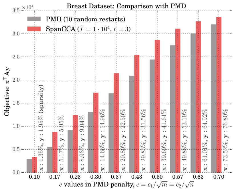
	Avg Exec. Time	Configuration
PMD	$\sim 44$ seconds	$10$ rand. restarts
SpanCCA	$\sim 24$ seconds	$T=10^{4}$, $r=3$.

Figure 1: Comparison of SpanCCA and the PMD algorithm (Witten et al., 2009). We configure PMD with $\ell_{1}$-norm thresholds $c_{1}=c\cdot\sqrt{m}$ and $c_{2}=c\cdot\sqrt{n}$, and consider various values of the constant $c\in(0,1)$. For each $c$, we run PMD $10$ times, select the canonical vectors $\mathbf{x}$, $\mathbf{y}$ that achieve the highest objective value and count their nonzero entries (depicted as percentage of the corresponding dimension). Finally, we run our SpanCCA algorithm with ${T=10^{4}}$ and ${r=3}$, using the latter as target sparsities, and compare the objective values achieved by the two methods. Execution times remain approximately the same for all target sparsity values (equiv. all $c$).

We run our algorithm on the breast cancer dataset and compare the output with the PMD algorithm of (Witten et al., 2009); PMD is regarded as state of the art by practitioners and has been used –in its original form or slightly modified– in several neuroscience and biomedical applications; see also Section 1.2. The input to both algorithms is the $m\times n$ matrix $\mathbf{\Sigma_{{\mathrm{X}\mathrm{Y}}}}=\mathbf{X}^{{\top}}\mathbf{Y}$ (${m=2149}$, ${n=19672}$), where $\mathbf{X}$ and $\mathbf{Y}$ are obtained from the aforementioned DNA and RNA matrices upon feature standardization. Recall that PMD is an iterative, alternating optimization scheme, where the sparsity of the extracted components $\mathbf{x}$ and $\mathbf{y}$ is implicitly controlled by enforcing upper bounds $c_{1}$ and $c_{2}$ on their $\ell_{1}$ norm, respectively, with $1\leq c_{1}\leq\sqrt{m}$ and $1\leq c_{2}\leq\sqrt{n}$. Here, for simplicity, we set ${c_{1}=c\sqrt{m}}$ and ${c_{2}=c\sqrt{n}}$ and consider multiple values of the constant $c$ in $(0,1)$. Note that under this configuration, for any given value of $c$, we expect that the extracted components will be approximately equally sparse, relatively to their dimension.

For each $c$, we first run the PMD algorithm $10$ times with random initializations, determine the pair of components $\mathbf{x}$ and $\mathbf{y}$ that achieves the highest objective value, and count the number of nonzero entries of both components as a percentage of their corresponding dimension. Subsequently, we run SpanCCA (Alg. 1) with parameters ${T=10^{4}}$, ${r=3}$, and target sparsity equal to that of the former PMD output. Recall that our algorithm administers precise control on the number of nonzero entries of the extracted components.

Figure 1 depicts the objective value achieved by the two algorithms, as well as the corresponding sparsity level of the extracted components. SpanCCA achieves a higher objective value in all cases. Finally, note that under the above configuration, both algorithms run for a few seconds per target sparsity, with SpanCCA running approximately half the time of PMD.

4.2 Brain Imaging Dataset

We analyzed functional statistical maps and behavioral variables from $497$ subjects available from the Human Connectome Project (HCP) (Van Essen et al., 2013). The HCP consists of high-quality imaging and behavioral data, collected from a large sample of healthy adult subjects, motivated by the goal of advancing knowledge between human brain function and its association to behavior. We apply our algorithm to investigate the shared co-variation between patterns of brain activity as measured by the experimental tasks, and behavioral variables. We selected the same subset of behavioral variables examined by (Smith et al., 2015), which include scores from psychological tests, physiological measurements, and self reported behavior questionnaires ($\mathbf{Y}$ dataset with dimensions $497\times 38$).

For each subject, we collected statistical maps corresponding to “$n$-back” task. These statistical maps summarize the activation of each voxel in response to the experimental manipulation. In the “$n$-back” task, designed to measure working memory, items are presented one at a time and subjects identify each item that repeats relative to the item that occurred $n$ items before. Further details on all tasks and variables are available in the HCP documentation (Van Essen et al., 2013).

We used the pre-computed 2back - 0back statistical contrast maps provided by the HCP. Standard preprocessing included motion correction, image registration to the MNI template (for comparison across subjects), and general linear model analysis, resulting in $91\times 109\times 91$ voxels. Voxels are then resampled to $61\times 73\times 61$ using the nilearn python package and applying standard brain masks, resulting in $65598$ voxels after masking non-grey matter regions. ($\mathbf{X}$ dataset with dimensions $497\times 65598$).

We apply our SpanCCA algorithm on the HCP data with arbitrarily selected parameters ${\mathrm{T}}=10^{6}$ and $r=5$. We set the target sparsity at $15\%$ for each canonical vector. Figure 2 depicts the brain regions and the behavioral factors corresponding to the nonzero weights of the extracted canonical pair. The map identifies a set of fronto-parietal regions known to be involved in executive function and working memory, which are the major functions isolated by the 2 back - 0-back contrast. In addition, it identifies deactivation in the default mode areas (medial prefrontal and parietal), which is also associated with engagement of difficult cognitive functions. The behavioral variables associated with activation of this network are all related to various aspects of intelligence; the Penn Matrix Reasoning Test (PMAT24, a measure of fluid intelligence), picture vocabulary (PicVocab, a measure of language comprehension), and reading ability (ReadEng).

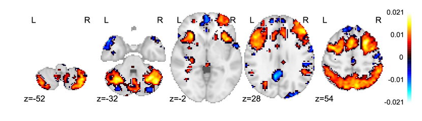
Behavioral Factor & Weight PMAT24_A_CR $0.487$ PicVocab_AgeAdj $0.448$ ReadEng_AgeAdj $0.440$ PicVocab_Unadj $0.433$ ReadEng_Unadj $0.426$

Figure 2: Brain regions and behavioral factors selected by the sparse left and right canonical vectors extracted by our SpanCCA algorithm. Target sparsity is set at $15\%$ for each canonical vector and SpanCCA is configured to run for ${\mathrm{T}}=10^{6}$ samples operating on a rank $r=5$ approximation of the input data. The map identifies a set of fronto-parietal regions known to be involved in executive function and working memory and deactivation in the default mode areas (medial prefrontal and parietal), which is also associated with engagement of difficult cognitive functions. The behavioral variables identified to be positively correlated with the activation of this network are all related to various aspects of intelligence.

Parallelization

To speed up execution, our prototypical Python implementation of SpanCCA exploits the multiprocessing module: $\mathrm{N}$ independent worker processes are spawned, and each one independently performs $\mathrm{T}/\mathrm{N}$ rounds of the main iteration of Alg. 1 returning a single canonical vector pair. The main process collects and compares the candidate pairs to determine the final output.

To demonstrate the parallelizability of our algorith, we run SpanCCA for the aforementioned task on the brain imaging data for various values of the number $\mathrm{N}$ of workers on a single server with $36$ physical processing cores and approximately $250\mathrm{Gb}$ of main memory. In Figure 3 (top panel), we plot the run time with respect to the number of workers used. The bottom panel depicts the achieved speedup factor: using the execution time on $5$ worker processes as a reference value, the speedup factor is the ratio of the execution time on $5$ processes over that on $\mathrm{N}$. As expected, the algorithm achieved a speedup factor that grows almost linearly in the number of available processors.

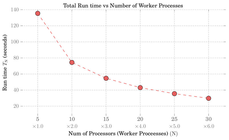
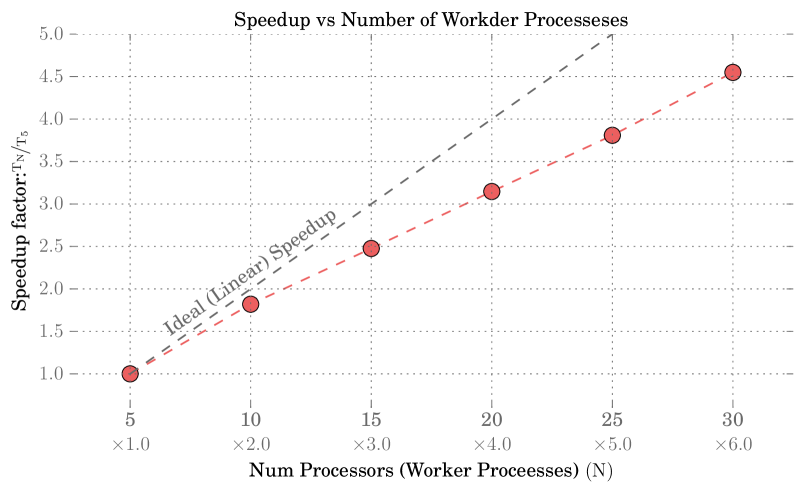
Figure 3: Speedup factors and corresponding total execution time, achieved by the prototypical parallel implementation of SpannCCA (Alg. 1) as a function of the number of worker processes or equivalently the number of processors used. Depicted values are medians over $20$ executions, each with ${T=10^{5}}$ and $r=5$, on the $65598\times 38$ example discussed in section 4.2. A speedup factory approximately linear in the number of workers is achieved.

5 Discussion

We presented a novel combinatorial algorithm for the sparse diagonal CCA problem and other constrained variants, with provable data-dependent global approximation guarantees and several attractive properties: the algorithm is simple, embarrassingly parallelizable, with complexity that scales linearly in the dimension of the input data, while it administers precise control on the sparsity of the extracted canonical vectors. Further it can accommodate additional structural constraints by plugging in a suitable “projection” subroutine.

Several directions remain open. We addressed the question of computing a single pair of sparse canonical vectors. Numerically, multiple pairs can be computed successively employing an appropriate deflation step. However, determining the kind of deflation most suitable for the application at hand, as well as the sparsity level of each component can be a challenging task, leaving a lot of room for research.

6 Hardness

We provide a proof for the NP-hardness of the constrained (and specifically sparse) CCA problem via a reduction from sparse PCA. Recall that sparse PCA is the following optimization problem:

$$\max_{\begin{subarray}{c}\mathbf{x}:\|\mathbf{x}\|_{0}=k\\ \|\mathbf{x}\|_{2}=1\end{subarray}}\mathbf{x}^{{\top}}\mathbf{A}\mathbf{x},$$ (13)

where $k$ is a given parameter and $\mathbf{A}$ a given $n\times n$ positive semidefinite (PSD) matrix.

We show that the sparse PCA problem (13) reduces to the sparse CCA problem (2) and in particular the maximization

$$\max_{\begin{subarray}{c}\mathbf{x}:\|\mathbf{x}\|_{0}=k,\|\mathbf{x}\|_{2}=1\\ \mathbf{y}:\|\mathbf{y}\|_{0}=k,\|\mathbf{y}\|_{2}=1\end{subarray}}\mathbf{x}^{{\top}}\mathbf{A}\mathbf{y}.$$ (14)

The only difference between (13) and (14) is that in the latter the optimal values for the two variables $\mathbf{x}$ and $\mathbf{y}$ may be different. If we add the constraint $\mathbf{x}=\mathbf{y}$ in  (14), then then two maximizations are identical. We show that this is not necessary: since $\mathbf{A}$ is PSD, the optimal solution of (14) will inherently satisfy $\mathbf{x}=\mathbf{y}$, and in turn the two maximizations are equivalent.

Let $\mathbf{U},\mathbf{\Lambda}$ be the eigenvalue decomposition of $\mathbf{A}$: the $n\times n$ matrix $\mathbf{U}$ contains the eigenvectors, while the $n\times n$ diagonal $\mathbf{\Lambda}$ contains the eigenvalues $\lambda_{1},\ldots,\lambda_{n}\geq 0$ in decreasing order. Let ($\mathbf{x}_{\star}$, $\mathbf{y}_{\star}$) be the optimal solution of (14). Further, let $\overline{\mathbf{x}}=\mathbf{U}^{{\top}}\mathbf{x}_{\star}$, and $\overline{\mathbf{y}}=\mathbf{U}^{{\top}}\mathbf{y}_{\star}$. Then,

$$\mathbf{x}_{\star}^{{\top}}\mathbf{A}\mathbf{y}_{\star}=\mathbf{x}_{\star}^{{\top}}\mathbf{U}\mathbf{\Lambda}\mathbf{U}^{{\top}}\mathbf{y}_{\star}=\overline{\mathbf{x}}^{{\top}}\mathbf{\Lambda}\overline{\mathbf{y}}=\sum_{i=1}^{n}\overline{x}_{i}\overline{y}_{i}\lambda_{i}.$$ (15)

Theorem 3 (Weighted Cauchy-Schwarz inequality; cvetkovski:inequalities, Theorem 10.1).

Let $a_{i},b_{i}\in\mathbb{R}$ be real numbers and let ${m_{i}\in\mathbb{R}^{+}}$, $i=1,2,\ldots,n$. Then,

$$\mathopen{}\mathclose{{}\left(\sum_{i=1}^{n}a_{i}b_{i}m_{i}}\right)^{2}\leq\mathopen{}\mathclose{{}\left(\sum_{i=1}^{n}a_{i}^{2}m_{i}}\right)\mathopen{}\mathclose{{}\left(\sum_{i=1}^{n}b_{i}^{2}m_{i}}\right).$$

Equality occurs if and only if $\tfrac{a_{1}}{b_{2}}=\ldots=\tfrac{a_{n}}{b_{n}}$.

By Theorem 3,

$$\mathopen{}\mathclose{{}\left(\mathbf{x}_{\star}^{{\top}}\mathbf{A}\mathbf{y}_{\star}}\right)^{2}\leq\mathopen{}\mathclose{{}\left(\sum_{i=1}^{n}\overline{x}_{i}^{2}\lambda_{i}}\right)\mathopen{}\mathclose{{}\left(\sum_{i=1}^{n}\overline{y}_{i}^{2}\lambda_{i}}\right),$$

with equality if and only if there exists a constant $c\in\mathbb{R}$ such that $\overline{\mathbf{x}}=c\cdot\overline{\mathbf{y}}$, and taking into account that both $\overline{\mathbf{x}}$ and $\overline{\mathbf{y}}$ are unit norm vectors, it follows that $\overline{\mathbf{x}}=\overline{\mathbf{y}}$. Finally, since $\mathbf{U}$ is a full rank matrix (in fact orthonormal basis of $\mathbb{R}^{n}$), it follows that $\mathbf{x}_{\star}=\mathbf{y}_{\star}$ must hold.

7 Proofs

For the remainder of this section, we define

$$\mathopen{}\mathclose{{}\left(\mathbf{u}_{\star},\mathbf{v}_{\star}}\right){\triangleq}\operatorname*{arg\,max}_{\mathbf{u}\in\mathcal{U},\mathbf{v}\in\mathcal{V}}\mathbf{u}^{{\top}}\mathbf{\Sigma_{{\mathrm{X}\mathrm{Y}}}}\mathbf{v},$$

i.e., $\mathbf{u}_{\star},\mathbf{v}_{\star}$ is a feasible pair that maximizes –not necessarily uniquely– the objective. Here, $\mathbf{\Sigma_{{\mathrm{X}\mathrm{Y}}}}$ is a given $m\times n$ real matrix, which plays the role of Further, we assume that there exists procedures to compute the exact soluton to $\mathsf{P}_{\mathcal{U}}(\cdot)$ and $\mathsf{P}_{\mathcal{V}}(\cdot)$ in (5) and (6), running in time $\mathrm{T}_{\mathcal{U}}$ and $\mathrm{T}_{\mathcal{V}}$, respectively. The following results can be easily adapted for the case where these procedures yield approximate solutions.

Lemma 7.3.

For any real ${m\times n}$ matrix $\mathbf{\Sigma_{{\mathrm{X}\mathrm{Y}}}}$ with $\text{rank}(\mathbf{\Sigma_{{\mathrm{X}\mathrm{Y}}}})=r\leq\max\{m,n\}$ and $\epsilon\in(0,1)$, Algorithm 1 with input $\mathbf{\Sigma_{{\mathrm{X}\mathrm{Y}}}}$, $r$, and $T=\widetilde{O}\bigl{(}2^{r\cdot\log_{2}(\nicefrac{{2}}{{\epsilon}})}\bigr{)}$ outputs $\mathbf{u}_{\sharp}\in\mathcal{U}$ and $\mathbf{v}_{\sharp}\in\mathcal{V}$ such that

$$\mathbf{u}_{\sharp}^{{\top}}\mathbf{\Sigma_{{\mathrm{X}\mathrm{Y}}}}\mathbf{v}_{\sharp}\geq\mathbf{u}_{\star}^{{\top}}\mathbf{\Sigma_{{\mathrm{X}\mathrm{Y}}}}\mathbf{v}_{\star}-\epsilon\cdot\sigma_{1}(\mathbf{\Sigma_{{\mathrm{X}\mathrm{Y}}}}),$$

in time $\mathrm{T}_{{\mathsf{SVD}}}(r)+O\mathopen{}\bigl{(}T\cdot\bigl{(}\mathrm{T}_{\mathcal{U}}+\mathrm{T}_{\mathcal{V}}+r\cdot\max\{m,n\}\bigr{)}\bigr{)}$.

Proof.

In the sequel, $\mathbf{U}$, $\mathbf{\Sigma}$ and $\mathbf{V}$ are used to denote the $r$-truncated singular value decomposition of $\mathbf{\Sigma_{{\mathrm{X}\mathrm{Y}}}}$. Note that the lemma assumes that the accuracy parameter $r$ is equal to the rank of the input matrix $\mathbf{\Sigma_{{\mathrm{X}\mathrm{Y}}}}$ and hence ${\mathbf{\Sigma_{{\mathrm{X}\mathrm{Y}}}}=\mathbf{U}\mathbf{\Sigma}\mathbf{V}^{{\top}}}$.

Recall that $\mathbf{u}_{\star},\mathbf{v}_{\star}$ is a pair —not necessarily unique— that maximizes the objective $\mathbf{u}^{{\top}}\mathbf{\Sigma_{{\mathrm{X}\mathrm{Y}}}}\mathbf{v}$ over all feasible solutions. Define $\mathbf{c}_{\star}{\triangleq}\mathbf{V}^{{\top}}\mathbf{v}_{\star}$. Note that $\mathbf{c}_{\star}$ is a vector in $\mathbf{R}^{r\times 1}$ with $\|\mathbf{c}_{\star}\|_{2}\leq 1$ since the $r$ columns of $\mathbf{V}$ are orthonormal and ${\|\mathbf{v}_{\star}\|_{2}=1}$. Finally, let $\overline{\mathbf{c}}_{\star}{\triangleq}\mathbf{c}_{\star}/\|\mathbf{c}_{\star}\|_{2}$. Note that $\|\mathbf{c}_{\star}\|_{2}>0$ since by assumption $\mathbf{u}_{\star}^{{\top}}\mathbf{\Sigma_{{\mathrm{X}\mathrm{Y}}}}\mathbf{v}_{\star}>0$.

Algorithm 1 operates in an iterative fashion. In each iteration, it independently considers a point $\mathbf{c}$ selected randomly and uniformly from the $r$-dimensional $\ell_{2}$-unit sphere $\mathbb{S}_{2}^{r-1}$ and generates a candidate solution pair at each point. For $\mathrm{T}=\widetilde{O}\bigl{(}2^{r\cdot\log_{2}(\nicefrac{{2}}{{\epsilon}})}\bigr{)}$, the collection of randomly sampled poins forms an $\nicefrac{{\epsilon}}{{2}}$-net for $\mathbb{S}_{2}^{r-1}$. By definition, the $\nicefrac{{\epsilon}}{{2}}$-net contains a point $\widetilde{\mathbf{c}}\in\mathbb{R}^{r\times 1}$, such that

$$\|\widetilde{\mathbf{c}}-\overline{\mathbf{c}}_{\star}\|_{2}\leq\epsilon/2.$$ (16)

Let $(\widetilde{\mathbf{u}},\widetilde{\mathbf{v}})$ be the candidate solution pair computed at $\widetilde{\mathbf{c}}$ by the two step maximization procedure, i.e., let

$$\widetilde{\mathbf{u}}\;{\triangleq}\;\operatorname*{arg\,max}_{\mathbf{u}\in\mathcal{U}}\mathbf{u}^{{\top}}\mathbf{U}\mathbf{\Sigma}\widetilde{\mathbf{c}}$$ (17)

and

$$\widetilde{\mathbf{v}}\;{\triangleq}\;\operatorname*{arg\,max}_{\mathbf{v}\in\mathcal{V}}\widetilde{\mathbf{u}}^{{\top}}\mathbf{\Sigma_{{\mathrm{X}\mathrm{Y}}}}\mathbf{v}.$$ (18)

By the definition of $\mathbf{c}_{\star}$, and letting $\rho{\triangleq}\|\mathbf{c}_{\star}\|_{2}$

$${\mathbf{u}}_{\star}^{{\top}}\mathbf{\Sigma_{{\mathrm{X}\mathrm{Y}}}}{\mathbf{v}}_{\star} =\mathbf{u}_{\star}^{{\top}}\mathbf{U}\mathbf{\Sigma}\mathbf{c}_{\star}$$

$$=\rho\cdot\mathbf{u}_{\star}^{{\top}}\mathbf{U}\mathbf{\Sigma}\overline{\mathbf{c}}_{\star}$$

$$=\rho\cdot\mathbf{u}_{\star}^{{\top}}\mathbf{U}\mathbf{\Sigma}\widetilde{\mathbf{c}}+\rho\cdot\mathbf{u}_{\star}^{{\top}}\mathbf{U}\mathbf{\Sigma}\bigl{(}\overline{\mathbf{c}}_{\star}-\widetilde{\mathbf{c}}\bigr{)}$$

$$\leq\rho\cdot\widetilde{\mathbf{u}}^{{\top}}\mathbf{U}\mathbf{\Sigma}\widetilde{\mathbf{c}}+\rho\cdot\mathbf{u}_{\star}^{{\top}}\mathbf{U}\mathbf{\Sigma}\bigl{(}\overline{\mathbf{c}}_{\star}-\widetilde{\mathbf{c}}\bigr{)}$$

$$\leq\rho\cdot\widetilde{\mathbf{u}}^{{\top}}\mathbf{U}\mathbf{\Sigma}\widetilde{\mathbf{c}}+\tfrac{\epsilon}{2}\cdot\sigma_{1}(\mathbf{\Sigma_{{\mathrm{X}\mathrm{Y}}}}).$$ (19)

The first inequality follows from the fact that $\widetilde{\mathbf{u}}$ by definition maximizes the first term over all $\mathbf{u}\in\mathcal{U}$. The last inequality is due to Lemma 8.8 and the fact that $\|\mathbf{u}_{\star}\|_{2}=1$ and $\rho\leq 1$. We further upper bound the right hand side of (19) as follows:

$$\rho\cdot\widetilde{\mathbf{u}}^{{\top}}\mathbf{U}\mathbf{\Sigma}\widetilde{\mathbf{c}}$$

$$=\rho\cdot\widetilde{\mathbf{u}}^{{\top}}\mathbf{U}\mathbf{\Sigma}\overline{\mathbf{c}}_{\star}+\rho\cdot\widetilde{\mathbf{u}}^{{\top}}\mathbf{U}\mathbf{\Sigma}\mathopen{}\mathclose{{}\left(\widetilde{\mathbf{c}}-\overline{\mathbf{c}}_{\star}}\right)$$

$$=\widetilde{\mathbf{u}}^{{\top}}\mathbf{U}\mathbf{\Sigma}\mathbf{c}_{\star}+\rho\cdot\widetilde{\mathbf{u}}^{{\top}}\mathbf{U}\mathbf{\Sigma}\mathopen{}\mathclose{{}\left(\widetilde{\mathbf{c}}-\overline{\mathbf{c}}_{\star}}\right)$$

$$=\widetilde{\mathbf{u}}^{{\top}}\mathbf{U}\mathbf{\Sigma}\mathbf{V}^{{\top}}\mathbf{v}_{\star}+\rho\cdot\widetilde{\mathbf{u}}^{{\top}}\mathbf{U}\mathbf{\Sigma}\mathopen{}\mathclose{{}\left(\widetilde{\mathbf{c}}-\overline{\mathbf{c}}_{\star}}\right)$$

$$\leq\widetilde{\mathbf{u}}^{{\top}}\mathbf{U}\mathbf{\Sigma}\mathbf{V}^{{\top}}\widetilde{\mathbf{v}}+\rho\cdot\widetilde{\mathbf{u}}^{{\top}}\mathbf{U}\mathbf{\Sigma}\mathopen{}\mathclose{{}\left(\widetilde{\mathbf{c}}-\overline{\mathbf{c}}_{\star}}\right)$$ (20)

$$\leq\widetilde{\mathbf{u}}^{{\top}}\mathbf{\Sigma_{{\mathrm{X}\mathrm{Y}}}}\widetilde{\mathbf{v}}+\tfrac{\epsilon}{2}\cdot\sigma_{1}(\mathbf{\Sigma_{{\mathrm{X}\mathrm{Y}}}}).$$ (21)

Inequality (20) follows by the fact that $\widetilde{\mathbf{v}}$ by definition (18) maximizes the bilinear term $\mathbf{u}^{{\top}}\mathbf{\Sigma_{{\mathrm{X}\mathrm{Y}}}}\mathbf{v}$ over all ${\mathbf{v}\in\mathcal{V}}$ when $\mathbf{u}=\widetilde{\mathbf{u}}$. The last inequality is once again due to Lemma 8.8 and the fact that $\|\mathbf{u}_{\star}\|_{2}=1$ and $\rho\leq 1$. Combining (19) and (21), we obtain

$$\widetilde{\mathbf{u}}^{{\top}}\mathbf{\Sigma_{{\mathrm{X}\mathrm{Y}}}}\widetilde{\mathbf{v}}\geq\mathbf{u}_{\star}^{{\top}}\mathbf{\Sigma_{{\mathrm{X}\mathrm{Y}}}}\mathbf{v}_{\star}-\epsilon\cdot\sigma_{1}(\mathbf{\Sigma_{{\mathrm{X}\mathrm{Y}}}}).$$

Algorithm 1 computes multiple candidate solution pairs and outputs the one that maximizes the objective. Therefore, the output pair $(\mathbf{u}_{\sharp},\mathbf{v}_{\sharp})$ must achieve a value as least as high as that achieved by $(\widetilde{\mathbf{u}},\widetilde{\mathbf{v}})$, which implies the desired guarantee.

The running time of Algorithm 1 follows straightforwardly by inspection. The algorithm first computes the truncated singular value decomposition of inner dimension $r$ in time denoted by $\mathrm{T}_{\texttt{SVD}}(r)$. Subsequently, it performs $T$ iterations. The cost of each iteration is determined by the cost of the matrix-vector multiplications and the running times $\mathrm{T}_{\mathcal{U}}$ and $\mathrm{T}_{\mathcal{V}}$ of the operators $\mathsf{P}_{\mathcal{U}}(\cdot)$ and $\mathsf{P}_{\mathcal{V}}(\cdot)$. Note that matrix multiplications can exploit the available singular value decomposition of $\mathbf{\Sigma_{{\mathrm{X}\mathrm{Y}}}}$ and are performed in time ${r\cdot\max\{m,n\}}$. Substituting the value of $\mathrm{T}$, completes the proof. ∎

Theorem 1.

For any real ${m\times n}$ matrix $\mathbf{\Sigma_{{\mathrm{X}\mathrm{Y}}}}$, $\epsilon\in(0,1)$, and $r\leq\max\{m,n\}$, Algorithm 1 with input $\mathbf{\Sigma_{{\mathrm{X}\mathrm{Y}}}}$, $r$, and $T=\widetilde{O}\bigl{(}2^{r\cdot\log_{2}(\nicefrac{{2}}{{\epsilon}})}\bigr{)}$ outputs $\mathbf{u}_{\sharp}\in\mathcal{U}$ and $\mathbf{v}_{\sharp}\in\mathcal{V}$ such that

$$\mathbf{u}_{\sharp}^{{\top}}\mathbf{\Sigma_{{\mathrm{X}\mathrm{Y}}}}\mathbf{v}_{\sharp}\geq\mathbf{u}_{\star}^{{\top}}\mathbf{\Sigma_{{\mathrm{X}\mathrm{Y}}}}\mathbf{v}_{\star}-\epsilon\cdot\sigma_{1}(\mathbf{\Sigma_{{\mathrm{X}\mathrm{Y}}}})-2\cdot\sigma_{r+1}(\mathbf{\Sigma_{{\mathrm{X}\mathrm{Y}}}}),$$

in time $\mathrm{T}_{{\mathsf{SVD}}}(r)+O\mathopen{}\bigl{(}T\cdot\bigl{(}\mathrm{T}_{\mathcal{U}}+\mathrm{T}_{\mathcal{V}}+r\cdot\max\{m,n\}\bigr{)}\bigr{)}$.

Proof.

Recall that Algorithm 1 with input an $m\times n$ matrix $\mathbf{\Sigma_{{\mathrm{X}\mathrm{Y}}}}$ and accuracy parameter $r$, first computes a rank-$r$ truncated singular value decomposition $\mathbf{U}$, $\mathbf{\Sigma}$, $\mathbf{V}$ and operates on that principal subspace of $\mathbf{\Sigma_{{\mathrm{X}\mathrm{Y}}}}$. Let $\mathbf{B}$ be the $m\times n$ best rank-$r$ approximation of $\mathbf{\Sigma_{{\mathrm{X}\mathrm{Y}}}}$ under the spectral norm. Then $\mathbf{B}=\mathbf{U}\mathbf{\Sigma}\mathbf{V}^{{\top}}$. One can easily verify that running Algorithm 1 with input $\mathbf{\Sigma_{{\mathrm{X}\mathrm{Y}}}}$ and accuracy parameter $r$, is equivalent to applying the algorithm on $\mathbf{B}$ with the same parameters.

By Lemma 7.3, Algorithm 1 outputs $\mathbf{u}_{\sharp},\mathbf{v}_{\sharp}$ such that

$$\mathbf{u}_{\sharp}^{{\top}}\mathbf{B}\mathbf{v}_{\sharp}\geq\widehat{\mathbf{u}}_{\star}^{{\top}}\mathbf{B}\widehat{\mathbf{v}}_{\star}-\epsilon\cdot\sigma_{1}(\mathbf{B}),$$ (22)

where

$$\mathopen{}\mathclose{{}\left(\widehat{\mathbf{u}}_{\star},\widehat{\mathbf{v}}_{\star}}\right){\triangleq}\operatorname*{arg\,max}_{\mathbf{u}\in\mathcal{U},\mathbf{v}\in\mathcal{V}}\mathbf{u}^{{\top}}\mathbf{B}\mathbf{v}$$

is a pair that optimally solves the maximization on the rank-$r$ matrix $\mathbf{B}$. By the optimality of the pair $\widehat{\mathbf{u}}_{\star},\widehat{\mathbf{v}}_{\star}$ for the rank-$r$ problem, it follows that

$$\widehat{\mathbf{u}}_{\star}^{{\top}}\mathbf{B}\widehat{\mathbf{v}}_{\star}\geq\mathbf{u}_{\star}^{{\top}}\mathbf{B}\mathbf{v}_{\star}.$$ (23)

Recall that $\mathbf{u}_{\star}$, $\mathbf{v}_{\star}$ is the pair that optimally solves the maximization on the original input matrix $\mathbf{\Sigma_{{\mathrm{X}\mathrm{Y}}}}$. Further,

$$\mathbf{u}_{\star}^{{\top}}\mathbf{B}\mathbf{v}_{\star} =\mathbf{u}_{\star}^{{\top}}\mathbf{\Sigma_{{\mathrm{X}\mathrm{Y}}}}\mathbf{v}_{\star}-\mathbf{u}_{\star}^{{\top}}(\mathbf{\Sigma_{{\mathrm{X}\mathrm{Y}}}}-\mathbf{B})\mathbf{v}_{\star}$$

$$\geq\mathbf{u}_{\star}^{{\top}}\mathbf{\Sigma_{{\mathrm{X}\mathrm{Y}}}}\mathbf{v}_{\star}-\bigl{\lvert}\mathbf{u}_{\star}^{{\top}}(\mathbf{\Sigma_{{\mathrm{X}\mathrm{Y}}}}-\mathbf{B})\mathbf{v}_{\star}\bigr{\rvert}$$

$$\geq\mathbf{u}_{\star}^{{\top}}\mathbf{\Sigma_{{\mathrm{X}\mathrm{Y}}}}\mathbf{v}_{\star}-\sigma_{r+1}(\mathbf{\Sigma_{{\mathrm{X}\mathrm{Y}}}}).$$ (24)

Combining (24) with (22) and (23),

$$\mathbf{u}_{\sharp}^{{\top}}\mathbf{B}\mathbf{v}_{\sharp}\geq\mathbf{u}_{\star}^{{\top}}\mathbf{\Sigma_{{\mathrm{X}\mathrm{Y}}}}\mathbf{v}_{\star}-\sigma_{r+1}(\mathbf{\Sigma_{{\mathrm{X}\mathrm{Y}}}})-\epsilon\cdot\sigma_{1}(\mathbf{B}).$$

Finally,

$$\mathbf{u}_{\sharp}^{{\top}}\mathbf{B}\mathbf{v}_{\sharp} =\mathbf{u}_{\sharp}^{{\top}}\mathbf{\Sigma_{{\mathrm{X}\mathrm{Y}}}}\mathbf{v}_{\sharp}-\mathbf{u}_{\sharp}^{{\top}}(\mathbf{\Sigma_{{\mathrm{X}\mathrm{Y}}}}-\mathbf{B})\mathbf{v}_{\sharp}$$

$$\leq\mathbf{u}_{\sharp}^{{\top}}\mathbf{\Sigma_{{\mathrm{X}\mathrm{Y}}}}\mathbf{v}_{\sharp}+\bigl{\lvert}\mathbf{u}_{\sharp}^{{\top}}(\mathbf{\Sigma_{{\mathrm{X}\mathrm{Y}}}}-\mathbf{B})\mathbf{v}_{\sharp}\bigr{\rvert}.$$

$$\leq\mathbf{u}_{\sharp}^{{\top}}\mathbf{\Sigma_{{\mathrm{X}\mathrm{Y}}}}\mathbf{v}_{\sharp}+\sigma_{r+1}(\mathbf{\Sigma_{{\mathrm{X}\mathrm{Y}}}}).$$ (25)

Combining with the previous inequality, we obtain

$$\mathbf{u}_{\sharp}^{{\top}}\mathbf{\Sigma_{{\mathrm{X}\mathrm{Y}}}}\mathbf{v}_{\sharp}\geq\mathbf{u}_{\star}^{{\top}}\mathbf{\Sigma_{{\mathrm{X}\mathrm{Y}}}}\mathbf{v}_{\star}-2\cdot\sigma_{r+1}(\mathbf{\Sigma_{{\mathrm{X}\mathrm{Y}}}})-\epsilon\cdot\sigma_{1}(\mathbf{B}).$$

Noting that ${\sigma_{1}(\mathbf{B})=\sigma_{1}(\mathbf{\Sigma_{{\mathrm{X}\mathrm{Y}}}})}$ completes the proof of the approximation guarantee. The running time of the algorithm is established in Lemma 7.3. ∎

Lemma 7.4.

For any real ${m\times n}$ matrix $\mathbf{\Sigma_{{\mathrm{X}\mathrm{Y}}}}$ with $\text{rank}(\mathbf{\Sigma_{{\mathrm{X}\mathrm{Y}}}})=r\leq\max\{m,n\}$ and $\epsilon\in(0,1)$, if $\mathcal{V}=\mathopen{}\mathclose{{}\left\{\mathbf{v}~{}:~{}\|\mathbf{v}\|_{2}=1}\right\}$, then Algorithm 1 with input $\mathbf{\Sigma_{{\mathrm{X}\mathrm{Y}}}}$, $r$, and $\mathrm{T}=\widetilde{O}\bigl{(}2^{r\cdot\log_{2}(\nicefrac{{2}}{{\epsilon}})}\bigr{)}$ outputs $\mathbf{u}_{\sharp}\in\mathcal{U}$ and $\mathbf{v}_{\sharp}\in\mathcal{V}$ such that

$$\mathbf{u}_{\sharp}^{{\top}}\mathbf{\Sigma_{{\mathrm{X}\mathrm{Y}}}}\mathbf{v}_{\sharp}\geq(1-\epsilon)\cdot\mathbf{u}_{\star}^{{\top}}\mathbf{\Sigma_{{\mathrm{X}\mathrm{Y}}}}\mathbf{v}_{\star}$$

in time $\mathrm{T}_{{\mathsf{SVD}}}(r)+O\mathopen{}\bigl{(}\mathrm{T}\cdot\bigl{(}\mathrm{T}_{\mathcal{U}}+\mathrm{T}_{\mathcal{V}}+r\cdot\max\{m,n\}\bigr{)}\bigr{)}$.

Proof.

The lemma focuses on the special case where the feasible region for the variable $\mathbf{v}$ coincides with the set of vectors with unit $\ell_{2}$ norm, i.e.,

$$\mathcal{V}=\{\mathbf{v}:\|\mathbf{v}\|_{2}=1\}.$$ (26)

The feasible region $\mathcal{U}$ for $\mathbf{u}$ is arbitrary, assuming once again that there exists an efficient operator $\mathsf{P}_{\mathcal{U}}(\cdot)$.

By the Cauchy-Schwarz inequality, for any $\mathbf{u}_{0}\in\mathbb{R}^{m\times 1}$,

$$\mathbf{u}_{0}^{{\top}}\mathbf{\Sigma_{{\mathrm{X}\mathrm{Y}}}}\mathbf{v} \leq\|\mathbf{u}_{0}^{{\top}}\mathbf{\Sigma_{{\mathrm{X}\mathrm{Y}}}}\|_{2},\quad\forall\mathbf{v}\in\mathcal{V}.$$ (27)

In fact, equality is achieved when $\mathbf{v}$ is aligned with $\mathbf{\Sigma_{{\mathrm{X}\mathrm{Y}}}}^{{\top}}\mathbf{u}_{0}$, i.e., for $\mathbf{v}=\mathbf{\Sigma_{{\mathrm{X}\mathrm{Y}}}}^{{\top}}\mathbf{u}_{0}/\|\mathbf{\Sigma_{{\mathrm{X}\mathrm{Y}}}}^{{\top}}\mathbf{u}_{0}\|_{2}\in\mathcal{V}$. In turn, for any $\mathbf{u}_{0}\in\mathbb{R}^{m\times 1}$,

$$\max_{\mathbf{v}\in\mathcal{V}}\mathbf{u}_{0}^{{\top}}\mathbf{\Sigma_{{\mathrm{X}\mathrm{Y}}}}\mathbf{v} =\mathbf{u}_{0}^{{\top}}\mathbf{\Sigma_{{\mathrm{X}\mathrm{Y}}}}\mathbf{\Sigma_{{\mathrm{X}\mathrm{Y}}}}^{{\top}}\mathbf{u}_{0}/\|\mathbf{\Sigma_{{\mathrm{X}\mathrm{Y}}}}^{{\top}}\mathbf{u}_{0}\|_{2}$$

$$=\|\mathbf{\Sigma_{{\mathrm{X}\mathrm{Y}}}}^{{\top}}\mathbf{u}_{0}\|_{2}$$

$$=\|\mathbf{V}\mathbf{\Sigma}\mathbf{U}^{{\top}}\mathbf{u}_{0}\|_{2}$$

$$=\|\mathbf{\Sigma}\mathbf{U}^{{\top}}\mathbf{u}_{0}\|_{2},$$ (28)

where the last equality follows from the fact that the $r$ columns of $\mathbf{V}$ are orthonormal.

We now proceed in a fashion very similar to that in the proof of Lemma 7.3. Recall that $\mathbf{u}_{\star},\mathbf{v}_{\star}$ is a pair that maximizes –not necessarily uniquely– the objective $\mathbf{u}^{{\top}}\mathbf{\Sigma_{{\mathrm{X}\mathrm{Y}}}}\mathbf{v}$ over all feasible solutions, and define $\mathbf{c}_{\star}{\triangleq}\mathbf{V}^{{\top}}\mathbf{v}_{\star}$. Note that here,

$$\mathbf{c}_{\star}{\triangleq}\mathbf{V}^{{\top}}\mathbf{v}_{\star} =\mathbf{V}^{{\top}}\mathbf{\Sigma_{{\mathrm{X}\mathrm{Y}}}}^{{\top}}\mathbf{u}_{\star}/\|\mathbf{\Sigma_{{\mathrm{X}\mathrm{Y}}}}^{{\top}}\mathbf{u}_{\star}\|_{2}$$

$$=\mathbf{\Sigma}\mathbf{U}^{{\top}}\mathbf{u}_{\star}/\|\mathbf{V}\mathbf{\Sigma}\mathbf{U}^{{\top}}\mathbf{u}_{\star}\|_{2}$$

$$=\mathbf{\Sigma}\mathbf{U}^{{\top}}\mathbf{u}_{\star}/\|\mathbf{\Sigma}\mathbf{U}^{{\top}}\mathbf{u}_{\star}\|_{2}$$ (29)

and hence, $\|\mathbf{c}_{\star}\|_{2}=1$. Following similar reasoning as in the proof of Lemma 7.3, Algorithm 1 considers a point $\widetilde{\mathbf{c}}\in\mathbb{R}^{r\times 1}$, such that

$$\|\widetilde{\mathbf{c}}-\overline{\mathbf{c}}_{\star}\|_{2}\leq\epsilon.$$

Let $(\widetilde{\mathbf{u}},\widetilde{\mathbf{v}})$ be the candidate solution pair computed at $\widetilde{\mathbf{c}}$ by the two step maximization procedure. We have,

$${\mathbf{u}}_{\star}^{{\top}}\mathbf{\Sigma_{{\mathrm{X}\mathrm{Y}}}}{\mathbf{v}}_{\star} =\mathbf{u}_{\star}^{{\top}}\mathbf{U}\mathbf{\Sigma}\mathbf{c}_{\star}$$

$$=\mathbf{u}_{\star}^{{\top}}\mathbf{U}\mathbf{\Sigma}\widetilde{\mathbf{c}}+\mathbf{u}_{\star}^{{\top}}\mathbf{U}\mathbf{\Sigma}\bigl{(}\mathbf{c}_{\star}-\widetilde{\mathbf{c}}\bigr{)}$$

$$\leq\widetilde{\mathbf{u}}^{{\top}}\mathbf{U}\mathbf{\Sigma}\widetilde{\mathbf{c}}+\|\mathbf{u}_{\star}^{{\top}}\mathbf{U}\mathbf{\Sigma}\|_{2}\|\mathbf{c}_{\star}-\widetilde{\mathbf{c}}\|_{2}$$

$$\leq\widetilde{\mathbf{u}}^{{\top}}\mathbf{U}\mathbf{\Sigma}\widetilde{\mathbf{c}}+\epsilon\cdot\|\mathbf{u}_{\star}^{{\top}}\mathbf{U}\mathbf{\Sigma}\|_{2}.$$ (30)

where the first inequality follows from the fact that $\widetilde{\mathbf{u}}$ by definition maximizes the first term at $\widetilde{\mathbf{c}}$ over all $\mathbf{u}\in\mathcal{U}$ and the Cauchy-Schwarz inequality. The key difference from the proof of Lemma 7.3, is that the term $\|\mathbf{u}_{\star}^{{\top}}\mathbf{U}\mathbf{\Sigma}\|_{2}$ in the right-hand side coincides with the optimal objective value ${\mathbf{u}}_{\star}^{{\top}}\mathbf{\Sigma_{{\mathrm{X}\mathrm{Y}}}}{\mathbf{v}}_{\star}$ as follows from (28). For comparison, note that in the proof of Lemma 7.3 it was loosely upper bounded by ${\sigma_{1}(\mathbf{\Sigma_{{\mathrm{X}\mathrm{Y}}}})}$. Continuing from (30),

$$\mathopen{}\mathclose{{}\left(1-\epsilon}\right)\cdot{\mathbf{u}}_{\star}^{{\top}}\mathbf{\Sigma_{{\mathrm{X}\mathrm{Y}}}}{\mathbf{v}}_{\star} \leq\widetilde{\mathbf{u}}^{{\top}}\mathbf{U}\mathbf{\Sigma}\widetilde{\mathbf{c}}.$$ (31)

But, once again by the Cauchy-Schwarz inequality,

$$\widetilde{\mathbf{u}}^{{\top}}\mathbf{U}\mathbf{\Sigma}\widetilde{\mathbf{c}} \leq\|\widetilde{\mathbf{u}}^{{\top}}\mathbf{U}\mathbf{\Sigma}\|_{2}\|\widetilde{\mathbf{c}}\|_{2}$$

$$=\|\widetilde{\mathbf{u}}^{{\top}}\mathbf{U}\mathbf{\Sigma}\|_{2}$$ (32)

and by (28),

$$\widetilde{\mathbf{u}}^{{\top}}\mathbf{U}\mathbf{\Sigma}\widetilde{\mathbf{c}} =\max_{\mathbf{v}\in\mathcal{V}}\widetilde{\mathbf{u}}^{{\top}}\mathbf{\Sigma_{{\mathrm{X}\mathrm{Y}}}}\mathbf{v}=\widetilde{\mathbf{u}}^{{\top}}\mathbf{\Sigma_{{\mathrm{X}\mathrm{Y}}}}\widetilde{\mathbf{v}}.$$ (33)

Combining (33) with (31),

$$\widetilde{\mathbf{u}}^{{\top}}\mathbf{\Sigma_{{\mathrm{X}\mathrm{Y}}}}\widetilde{\mathbf{v}}\geq(1-\epsilon)\cdot\mathbf{u}_{\star}^{{\top}}\mathbf{\Sigma_{{\mathrm{X}\mathrm{Y}}}}\mathbf{v}_{\star}$$ (34)

Recalling that Algorithm 1 outputs the candidate pair that maximizes the objective among all computed feasible points implies the desired result. ∎

Theorem 2.

For any real ${m\times n}$ matrix $\mathbf{\Sigma_{{\mathrm{X}\mathrm{Y}}}}$ and $\epsilon\in(0,1)$, if $\mathcal{V}=\mathopen{}\mathclose{{}\left\{\mathbf{v}~{}:~{}\|\mathbf{v}\|_{2}=1}\right\}$, then Algorithm 1 with input $\mathbf{\Sigma_{{\mathrm{X}\mathrm{Y}}}}$, $r$, and $T=\widetilde{O}\bigl{(}2^{r\cdot\log_{2}(\nicefrac{{2}}{{\epsilon}})}\bigr{)}$ outputs $\mathbf{u}_{\sharp}\in\mathcal{U}$ and $\mathbf{v}_{\sharp}\in\mathcal{V}$ such that

$$\mathbf{u}_{\sharp}^{{\top}}\mathbf{\Sigma_{{\mathrm{X}\mathrm{Y}}}}\mathbf{v}_{\sharp}\geq(1-\epsilon)\cdot\mathbf{u}_{\star}^{{\top}}\mathbf{\Sigma_{{\mathrm{X}\mathrm{Y}}}}\mathbf{v}_{\star}-2\cdot\sigma_{r+1}(\mathbf{\Sigma_{{\mathrm{X}\mathrm{Y}}}})$$

in time $\mathrm{T}_{{\mathsf{SVD}}}(r)+O\mathopen{}\bigl{(}T\cdot\bigl{(}\mathrm{T}_{\mathcal{U}}+\mathrm{T}_{\mathcal{V}}+r\cdot\max\{m,n\}\bigr{)}\bigr{)}$.

Proof.

The Theorem follows from Lemma 7.4. The proof is similar to that of Theorem 1. The main difference lies in substituting (22) with

$$\mathbf{u}_{\sharp}^{{\top}}\mathbf{B}\mathbf{v}_{\sharp}\geq(1-\epsilon)\cdot\mathbf{u}_{{(B)}\star}^{{\top}}\mathbf{B}\mathbf{v}_{{(B)}\star}.$$ (35)

The remainder of the proof easily follows. ∎

8 Auxiliary Lemmata

Lemma 8.5.

Let $a_{1},\ldots,a_{n}$ and $b_{1},\ldots,b_{n}$ be $2n$ real numbers and let $p$ and $q$ be two numbers such that ${1/p}+{1/q}=1$ and $p>1$. We have

$$\bigl{\lvert}\sum_{i=1}^{n}a_{i}b_{i}\bigr{\rvert}\leq\bigl{(}\sum_{i=1}^{n}\lvert a_{i}\rvert^{p}\bigr{)}^{1/p}\cdot\bigl{(}\sum_{i=1}^{n}\lvert b_{i}\rvert^{q}\bigr{)}^{1/q}.$$

Lemma 8.6.

For any $\mathbf{A},\mathbf{B}\in\mathbb{R}^{n\times k}$,

$$\bigl{\lvert}\langle\mathbf{A},\mathbf{B}\rangle\bigr{\rvert}{\triangleq}\bigl{\lvert}{\textsc{Tr}}\bigl{(}\mathbf{A}^{{\top}}\mathbf{B}\bigr{)}\bigr{\rvert}\leq\|\mathbf{A}\|_{{\textnormal{\tiny{F}}}}\|\mathbf{B}\|_{{\textnormal{\tiny{F}}}}.$$

Proof.

Treating $\mathbf{A}$ and $\mathbf{B}$ as vectors, the lemma follows immediately from Lemma 8.5 for $p=q=2$. ∎

Lemma 8.7.

For any two real matrices $\mathbf{A}$ and $\mathbf{B}$ of appropriate dimensions,

$$\|\mathbf{A}\mathbf{B}\|_{{\textnormal{\tiny{F}}}}\leq\min\mathopen{}\bigl{\{}\|\mathbf{A}\|_{2}\|\mathbf{B}\|_{{\textnormal{\tiny{F}}}},\;\|\mathbf{A}\|_{{\textnormal{\tiny{F}}}}\|\mathbf{B}\|_{2}\bigr{\}}.$$

Proof.

Let $\mathbf{b}_{i}$ denote the $i$th column of $\mathbf{B}$. Then,

$$\|\mathbf{A}\mathbf{B}\|_{{\textnormal{\tiny{F}}}}^{2} =\sum_{i}\|\mathbf{A}\mathbf{b}_{i}\|_{2}^{2}\leq\sum_{i}\|\mathbf{A}\|_{2}^{2}\|\mathbf{b}_{i}\|_{2}^{2}$$

$$=\|\mathbf{A}\|_{2}^{2}\sum_{i}\|\mathbf{b}_{i}\|_{2}^{2}=\|\mathbf{A}\|_{2}^{2}\|\mathbf{B}\|_{{\textnormal{\tiny{F}}}}^{2}.$$

Similarly, using the previous inequality,

$$\|\mathbf{A}\mathbf{B}\|_{{\textnormal{\tiny{F}}}}^{2}=\|\mathbf{B}^{{\top}}\mathbf{A}^{{\top}}\|_{{\textnormal{\tiny{F}}}}^{2}\leq\|\mathbf{B}^{{\top}}\|_{2}^{2}\|\mathbf{A}^{{\top}}\|_{{\textnormal{\tiny{F}}}}^{2}=\|\mathbf{B}\|_{2}^{2}\|\mathbf{A}\|_{{\textnormal{\tiny{F}}}}^{2}.$$

The desired result follows combining the two upper bounds. ∎

Lemma 8.8.

For any real $m\times k$ matrix $\mathbf{X}$, $m\times n$ matrix $\mathbf{A}$, and $n\times k$ matrix $\mathbf{Y}$,

$$\bigl{\lvert}{\textsc{Tr}}\bigl{(}\mathbf{X}^{{\top}}\mathbf{A}\mathbf{Y}\bigr{)}\bigr{\rvert}\leq\|\mathbf{X}\|_{{\textnormal{\tiny{F}}}}\cdot\|\mathbf{A}\|_{2}\cdot\|\mathbf{Y}\|_{{\textnormal{\tiny{F}}}}.$$

Proof.

We have

$$\bigl{\lvert}{\textsc{Tr}}\bigl{(}\mathbf{X}^{{\top}}\mathbf{A}\mathbf{Y}\bigr{)}\bigr{\rvert}\leq\|\mathbf{X}\|_{{\textnormal{\tiny{F}}}}\cdot\|\mathbf{A}\mathbf{Y}\|_{{\textnormal{\tiny{F}}}}\leq\|\mathbf{X}\|_{{\textnormal{\tiny{F}}}}\cdot\|\mathbf{A}\|_{2}\cdot\|\mathbf{Y}\|_{{\textnormal{\tiny{F}}}},$$

with the first inequality following from Lemma 8.6 on $\lvert\langle\mathbf{X},\,\mathbf{A}\mathbf{Y}\rangle\rvert$ and the second from Lemma 8.7. ∎

Lemma 8.9.

For any real $m\times n$ matrix $\mathbf{A}$, and pair of $m\times k$ matrix $\mathbf{X}$ and $n\times k$ matrix $\mathbf{Y}$ such that $\mathbf{X}^{{\top}}\mathbf{X}=\mathbf{I}_{k}$ and $\mathbf{Y}^{{\top}}\mathbf{Y}=\mathbf{I}_{k}$ with $k\leq\min\{{m},\;{n}\}$, the following holds:

$$\bigl{\lvert}{\textsc{Tr}}\bigl{(}\mathbf{X}^{{\top}}\mathbf{A}\mathbf{Y}\bigr{)}\bigr{\rvert}\leq\sqrt{k}\cdot\bigl{(}\sum_{i=1}^{k}\sigma_{i}^{2}\bigl{(}\mathbf{A}\bigr{)}\bigr{)}^{1/2}.$$

Proof.

By Lemma 8.6,

$$\lvert\langle\mathbf{X},\,\mathbf{A}\mathbf{Y}\rangle\rvert =\bigl{\lvert}{\textsc{Tr}}\bigl{(}\mathbf{X}^{{\top}}\mathbf{A}\mathbf{Y}\bigr{)}\bigr{\rvert}$$

$$\leq\|\mathbf{X}\|_{{\textnormal{\tiny{F}}}}\cdot\|\mathbf{A}\mathbf{Y}\|_{{\textnormal{\tiny{F}}}}=\sqrt{k}\cdot\|\mathbf{A}\mathbf{Y}\|_{{\textnormal{\tiny{F}}}}.$$

where the last inequality follows from the fact that $\|\mathbf{X}\|_{{\textnormal{\tiny{F}}}}^{2}={\textsc{Tr}}\bigl{(}\mathbf{X}^{{\top}}\mathbf{X}\bigr{)}={\textsc{Tr}}\bigl{(}\mathbf{I}_{k}\bigr{)}=k$. Further, for any $\mathbf{Y}$ such that $\mathbf{Y}^{T}\mathbf{Y}=\mathbf{I}_{k}$,

$$\|\mathbf{A}\mathbf{Y}\|_{{\textnormal{\tiny{F}}}}^{2}\leq\max_{\begin{subarray}{c}\widehat{\mathbf{Y}}\in\mathbb{R}^{n\times k}\\ \widehat{\mathbf{Y}}^{{\top}}\widehat{\mathbf{Y}}=\mathbf{I}_{k}\end{subarray}}\|\mathbf{A}\widehat{\mathbf{Y}}\|_{{\textnormal{\tiny{F}}}}^{2}=\sum_{i=1}^{k}\sigma_{i}^{2}(\mathbf{A}).$$ (36)

Combining the two inequalities, the result follows. ∎

Lemma 8.10.

For any real $m\times n$ matrix $\mathbf{A}$, and any $k\leq\min\{{m},\;{n}\}$,

$$\max_{\begin{subarray}{c}{\mathbf{Y}}\in\mathbb{R}^{n\times k}\\ {\mathbf{Y}}^{{\top}}{\mathbf{Y}}=\mathbf{I}_{k}\end{subarray}}\|\mathbf{A}{\mathbf{Y}}\|_{{\textnormal{\tiny{F}}}}=\mathopen{}\mathclose{{}\left(\sum_{i=1}^{k}\sigma_{i}^{2}(\mathbf{A})}\right)^{1/2}.$$

The above equality is realized when the $k$ columns of $\mathbf{Y}$ coincide with the $k$ leading right singular vectors of $\mathbf{A}$.

Proof.

Let $\mathbf{U}\mathbf{\Sigma}\mathbf{V}^{{\top}}$ be the singular value decomposition of $\mathbf{A}$; $\mathbf{U}$ and $\mathbf{V}$ are $m\times m$ and $n\times n$ unitary matrices respectively, while $\Sigma$ is a diagonal matrix with $\Sigma_{jj}=\sigma_{j}$, the $j$th largest singular value of $\mathbf{A}$, $j=1,\ldots,d$, where $d{\triangleq}\min\{{m},{n}\}$. Due to the invariance of the Frobenius norm under unitary multiplication,

$$\|\mathbf{A}\mathbf{Y}\|_{{\textnormal{\tiny{F}}}}^{2}=\|\mathbf{U}\mathbf{\Sigma}\mathbf{V}^{{\top}}\mathbf{Y}\|_{{\textnormal{\tiny{F}}}}^{2}=\|\mathbf{\Sigma}\mathbf{V}^{{\top}}\mathbf{Y}\|_{{\textnormal{\tiny{F}}}}^{2}.$$ (37)

Continuing from (37),

$$\|\mathbf{\Sigma}\mathbf{V}^{{\top}}\mathbf{Y}\|_{{\textnormal{\tiny{F}}}}^{2} ={\textsc{Tr}}\bigl{(}\mathbf{Y}^{{\top}}\mathbf{V}\mathbf{\Sigma}^{2}\mathbf{V}^{{\top}}\mathbf{Y}\bigr{)}$$

$$=\sum_{i=1}^{k}\mathbf{y}_{i}^{{\top}}\mathopen{}\mathclose{{}\left(\sum_{j=1}^{d}\sigma_{j}^{2}\cdot\mathbf{v}_{j}\mathbf{v}_{j}^{{\top}}}\right)\mathbf{y}_{i}$$

$$=\sum_{j=1}^{d}\sigma_{j}^{2}\cdot\sum_{i=1}^{k}\mathopen{}\mathclose{{}\left(\mathbf{v}_{j}^{{\top}}\mathbf{y}_{i}}\right)^{2}.$$

Let $z_{j}{\triangleq}\sum_{i=1}^{k}\bigl{(}\mathbf{v}_{j}^{{\top}}\mathbf{y}_{i}\bigr{)}^{2}$, $j=1,\ldots,d$. Note that each individual $z_{j}$ satisfies

$$0\leq z_{j}{\triangleq}\sum_{i=1}^{k}\bigl{(}\mathbf{v}_{j}^{{\top}}\mathbf{y}_{i}\bigr{)}^{2}\leq\|\mathbf{v}_{j}\|^{2}=1,$$

where the last inequality follows from the fact that the columns of $\mathbf{Y}$ are orthonormal. Further,

$$\sum_{j=1}^{d}z_{j} =\sum_{j=1}^{d}\sum_{i=1}^{k}\bigl{(}\mathbf{v}_{j}^{{\top}}\mathbf{y}_{i}\bigr{)}^{2}=\sum_{i=1}^{k}\sum_{j=1}^{d}\bigl{(}\mathbf{v}_{j}^{{\top}}\mathbf{y}_{i}\bigr{)}^{2}$$

$$=\sum_{i=1}^{k}\|\mathbf{y}_{i}\|^{2}=k.$$

Combining the above, we conclude that

$$\|\mathbf{A}\mathbf{Y}\|_{{\textnormal{\tiny{F}}}}^{2}=\sum_{j=1}^{d}\sigma_{j}^{2}\cdot z_{j}\leq\sigma_{1}^{2}+\ldots+\sigma_{k}^{2}.$$ (38)

Finally, it is straightforward to verify that if $\mathbf{y}_{i}=\mathbf{v}_{i}$, $i=1,\ldots,k$, then (38) holds with equality. ∎

cca icml2016

References

• Amini & Wainwright (2008) Amini, Arash A and Wainwright, Martin J. High-dimensional analysis of semidefinite relaxations for sparse principal components. In Information Theory, 2008. ISIT 2008. IEEE International Symposium on, pp.  2454–2458. IEEE, 2008.
• Asteris et al. (2014) Asteris, Megasthenis, Papailiopoulos, Dimitris, and Dimakis, Alexandros. Nonnegative sparse PCA with provable guarantees. In Proceedings of the 31st International Conference on Machine Learning (ICML-14), pp.  1728–1736, 2014.
• Asteris et al. (2015) Asteris, Megasthenis, Kyrillidis, Anastasios, Dimakis, Alex, Yi, Han-Gyol, and Chandrasekaran, Bharath. Stay on path: Pca along graph paths. In Proceedings of the 32nd International Conference on Machine Learning (ICML-15), volume 37. JMLR Workshop and Conference Proceedings, 2015.
• Bach et al. (2012) Bach, Francis, Jenatton, Rodolphe, Mairal, Julien, Obozinski, Guillaume, et al. Structured sparsity through convex optimization. Statistical Science, 27(4):450–468, 2012.
• Baldassarre et al. (2013) Baldassarre, Luca, Bhan, Nirav, Cevher, Volkan, Kyrillidis, Anastasios, and Satpathi, Siddhartha. Group-sparse model selection: Hardness and relaxations. arXiv preprint arXiv:1303.3207, 2013.
• Baraniuk et al. (2010) Baraniuk, Richard G, Cevher, Volkan, Duarte, Marco F, and Hegde, Chinmay. Model-based compressive sensing. Information Theory, IEEE Transactions on, 56(4):1982–2001, 2010.
• Berman et al. (2006) Berman, Marc G, Jonides, John, and Nee, Derek Evan. Studying mind and brain with fmri. Social cognitive and affective neuroscience, 1(2):158–161, 2006.
• Chen et al. (2013) Chen, Jun, Bushman, Frederic D, Lewis, James D, Wu, Gary D, and Li, Hongzhe. Structure-constrained sparse canonical correlation analysis with an application to microbiome data analysis. Biostatistics, 14(2):244–258, 2013.
• Chen et al. (2012) Chen, Xi, Liu, Han, and Carbonell, Jaime G. Structured sparse canonical correlation analysis. In International Conference on Artificial Intelligence and Statistics, pp.  199–207, 2012.
• Chin et al. (2006) Chin, Koei, DeVries, Sandy, Fridlyand, Jane, Spellman, Paul T, Roydasgupta, Ritu, Kuo, Wen-Lin, Lapuk, Anna, Neve, Richard M, Qian, Zuwei, Ryder, Tom, et al. Genomic and transcriptional aberrations linked to breast cancer pathophysiologies. Cancer cell, 10(6):529–541, 2006.
• Chu et al. (2013) Chu, Delin, Liao, Li-Zhi, Ng, Michael K, and Zhang, Xiaowei. Sparse canonical correlation analysis: new formulation and algorithm. Pattern Analysis and Machine Intelligence, IEEE Transactions on, 35(12):3050–3065, 2013.
• d’Aspremont et al. (2007) d’Aspremont, Alexandre, El Ghaoui, Laurent, Jordan, Michael I, and Lanckriet, Gert RG. A direct formulation for sparse pca using semidefinite programming. SIAM review, 49(3):434–448, 2007.
• Deleus & Van Hulle (2011) Deleus, Filip and Van Hulle, Marc M. Functional connectivity analysis of fmri data based on regularized multiset canonical correlation analysis. Journal of Neuroscience methods, 197(1):143–157, 2011.
• Du et al. (2014) Du, Lei, Yan, Jingwen, Kim, Sungeun, Risacher, Shannon L, Huang, Heng, Inlow, Mark, Moore, Jason H, Saykin, Andrew J, and Shen, Li. A novel structure-aware sparse learning algorithm for brain imaging genetics. In Medical Image Computing and Computer-Assisted Intervention, pp.  329–336. Springer, 2014.
• Dudoit et al. (2002) Dudoit, Sandrine, Fridlyand, Jane, and Speed, Terence P. Comparison of discrimination methods for the classification of tumors using gene expression data. Journal of the American statistical association, 97(457):77–87, 2002.
• Halko et al. (2011) Halko, Nathan, Martinsson, Per-Gunnar, and Tropp, Joel A. Finding structure with randomness: Probabilistic algorithms for constructing approximate matrix decompositions. SIAM review, 53(2):217–288, 2011.
• Hardoon & Shawe-Taylor (2007) Hardoon, David R and Shawe-Taylor, John. Technical report, university college london (ucl). 2007.
• Hardoon & Shawe-Taylor (2011) Hardoon, David R and Shawe-Taylor, John. Sparse canonical correlation analysis. Machine Learning, 83(3):331–353, 2011.
• Hegde et al. (2015) Hegde, Chinmay, Indyk, Piotr, and Schmidt, Ludwig. A nearly-linear time framework for graph-structured sparsity. In Proceedings of The 32nd International Conference on Machine Learning, pp.  928–937, 2015.
• Hotelling (1936) Hotelling, Harold. Relations between two sets of variates. Biometrika, pp.  321–377, 1936.
• Huang et al. (2011) Huang, Junzhou, Zhang, Tong, and Metaxas, Dimitris. Learning with structured sparsity. The Journal of Machine Learning Research, 12:3371–3412, 2011.
• Kobayashi (2014) Kobayashi, Takumi. S3cca: Smoothly structured sparse cca for partial pattern matching. In Pattern Recognition (ICPR), 22nd International Conference on, pp.  1981–1986. IEEE, 2014.
• Kyrillidis & Cevher (2012) Kyrillidis, Anastasios and Cevher, Volkan. Combinatorial selection and least absolute shrinkage via the clash algorithm. In Information Theory Proceedings (ISIT), 2012 IEEE International Symposium on, pp.  2216–2220. IEEE, 2012.
• Kyrillidis et al. (2012) Kyrillidis, Anastasios, Puy, Gilles, and Cevher, Volkan. Hard thresholding with norm constraints. In 2012 IEEE International Conference on Acoustics, Speech and Signal Processing (ICASSP), number EPFL-CONF-183061, pp.  3645–3648. Ieee, 2012.
• Kyrillidis et al. (2015) Kyrillidis, Anastasios, Baldassarre, Luca, El Halabi, Marwa, Tran-Dinh, Quoc, and Cevher, Volkan. Structured sparsity: Discrete and convex approaches. In Compressed Sensing and its Applications, pp.  341–387. Springer, 2015.
• Lee et al. (2010) Lee, Mihee, Shen, Haipeng, Huang, Jianhua Z, and Marron, JS. Biclustering via sparse singular value decomposition. Biometrics, 66(4):1087–1095, 2010.
• Li et al. (2012) Li, Yi-Ou, Eichele, Tom, Calhoun, Vince D, and Adali, Tulay. Group study of simulated driving fmri data by multiset canonical correlation analysis. Journal of signal processing systems, 68(1):31–48, 2012.
• Lin et al. (2014) Lin, Dongdong, Calhoun, Vince D, and Wang, Yu-Ping. Correspondence between fmri and snp data by group sparse canonical correlation analysis. Medical image analysis, 18(6):891–902, 2014.
• Morley et al. (2004) Morley, Michael, Molony, Cliona M, Weber, Teresa M, Devlin, James L, Ewens, Kathryn G, Spielman, Richard S, and Cheung, Vivian G. Genetic analysis of genome-wide variation in human gene expression. Nature, 430(7001):743–747, 2004.
• Parkhomenko et al. (2009) Parkhomenko, Elena, Tritchler, David, and Beyene, Joseph. Sparse canonical correlation analysis with application to genomic data integration. Statistical Applications in Genetics and Molecular Biology, 8(1):1–34, 2009.
• Poldrack (2006) Poldrack, Russell A. Can cognitive processes be inferred from neuroimaging data? Trends in cognitive sciences, 10(2):59–63, 2006.
• Pollack et al. (2002) Pollack, Jonathan R, Sørlie, Therese, Perou, Charles M, Rees, Christian A, Jeffrey, Stefanie S, Lonning, Per E, Tibshirani, Robert, Botstein, David, Børresen-Dale, Anne-Lise, and Brown, Patrick O. Microarray analysis reveals a major direct role of dna copy number alteration in the transcriptional program of human breast tumors. Proceedings of the National Academy of Sciences, 99(20):12963–12968, 2002.
• Posner et al. (1988) Posner, Michael I, Petersen, Steven E, Fox, Peter T, and Raichle, Marcus E. Localization of cognitive operations in the human brain. Science, 240(4859):1627–1631, 1988.
• Rustandi et al. (2009) Rustandi, Indrayana, Just, Marcel Adam, and Mitchell, Tom. Integrating multiple-study multiple-subject fmri datasets using canonical correlation analysis. In Proceedings of the MICCAI 2009 Workshop: Statistical modeling and detection issues in intra-and inter-subject functional MRI data analysis, 2009.
• Smith et al. (2015) Smith, Stephen M, Nichols, Thomas E, Vidaurre, Diego, Winkler, Anderson M, Behrens, Timothy EJ, Glasser, Matthew F, Ugurbil, Kamil, Barch, Deanna M, Van Essen, David C, and Miller, Karla L. A positive-negative mode of population covariation links brain connectivity, demographics and behavior. Nature neuroscience, 18(11):1565–1567, 2015.
• Sriperumbudur et al. (2009) Sriperumbudur, Bharath, Torres, David, and Lanckriet, Gert. A DC programming approach to the sparse generalized eigenvalue problem. arXiv preprint arXiv:0901.1504, 2009.
• Stranger et al. (2007) Stranger, Barbara E, Forrest, Matthew S, Dunning, Mark, Ingle, Catherine E, Beazley, Claude, Thorne, Natalie, Redon, Richard, Bird, Christine P, de Grassi, Anna, Lee, Charles, et al. Relative impact of nucleotide and copy number variation on gene expression phenotypes. Science, 315(5813):848–853, 2007.
• Thompson (1984) Thompson, Bruce. Canonical correlation analysis: Uses and interpretation. Number 47. Sage, 1984.
• Thorndike (1976) Thorndike, Robert M. Correlational procedures for research. Wiley, 1976.
• Tibshirani et al. (2003) Tibshirani, Robert, Hastie, Trevor, Narasimhan, Balasubramanian, and Chu, Gilbert. Class prediction by nearest shrunken centroids, with applications to dna microarrays. Statistical Science, pp.  104–117, 2003.
• Torres et al. (2007) Torres, David A, Turnbull, Douglas, Barrington, Luke, and Lanckriet, Gert RG. Identifying words that are musically meaningful. In ISMIR, volume 7, pp.  405–410, 2007.
• Van Essen et al. (2013) Van Essen, David C, Smith, Stephen M, Barch, Deanna M, Behrens, Timothy EJ, Yacoub, Essa, Ugurbil, Kamil, Consortium, WU-Minn HCP, et al. The wu-minn human connectome project: an overview. Neuroimage, 80:62–79, 2013.
• Vershynin (2010) Vershynin, Roman. Introduction to the non-asymptotic analysis of random matrices. arXiv preprint arXiv:1011.3027, 2010.
• Waaijenborg et al. (2008) Waaijenborg, Sandra, Verselewel de Witt Hamer, Philip C, and Zwinderman, Aeilko H. Quantifying the association between gene expressions and dna-markers by penalized canonical correlation analysis. Statistical Applications in Genetics and Molecular Biology, 7(1), 2008.
• Wiesel et al. (2008) Wiesel, Ami, Kliger, Mark, and Hero III, Alfred O. A greedy approach to sparse canonical correlation analysis. arXiv preprint arXiv:0801.2748, 2008.
• Witten & Tibshirani (2009) Witten, Daniela M and Tibshirani, Robert J. Extensions of sparse canonical correlation analysis with applications to genomic data. Statistical applications in genetics and molecular biology, 8(1):1–27, 2009.
• Witten et al. (2009) Witten, Daniela M, Tibshirani, Robert, and Hastie, Trevor. A penalized matrix decomposition, with applications to sparse principal components and canonical correlation analysis. Biostatistics, pp.  kxp008, 2009.
• Yang et al. (2011) Yang, Dan, Ma, Zongming, and Buja, Andreas. A sparse SVD method for high-dimensional data. arXiv preprint arXiv:1112.2433, 2011.
• Zou & Hastie (2005) Zou, Hui and Hastie, Trevor. Regularization and variable selection via the elastic net. Journal of the Royal Statistical Society: Series B (Statistical Methodology), 67(2):301–320, 2005.
• Zou et al. (2006) Zou, Hui, Hastie, Trevor, and Tibshirani, Robert. Sparse principal component analysis. Journal of computational and graphical statistics, 15(2):265–286, 2006.