Singular ridge regression with homoscedastic residuals: generalization error with estimated parameters

Abstract

This paper characterizes the conditional distribution properties of the finite sample ridge regression estimator and uses that result to evaluate total regression and generalization errors that incorporate the inaccuracies committed at the time of parameter estimation. The paper provides explicit formulas for those errors. Unlike other classical references in this setup, our results take place in a fully singular setup that does not assume the existence of a solution for the non-regularized regression problem. In exchange, we invoke a conditional homoscedasticity hypothesis on the regularized regression residuals that is crucial in our developments.

Key Words: ridge regression, singular regression, training error, testing error, generalization error, regularization methods, high-dimensional regression.

1 Introduction

The ridge regression [Tikh 43, Tikh 63, Hoer 70] has been introduced as a regularization method to estimate the unknown matrix $B$ in the linear regression model $\mathbf{y}=B^{\top}\mathbf{x}+\boldsymbol{\varepsilon},$ when the covariance matrix of the explanatory variables $\Sigma_{\bf x}:={\rm Cov}({\bf x},{\bf x})\in\mathbb{S}_{p}$ is singular or poorly conditioned and, therefore, the standard least squares estimator is ill-defined. The ridge regularization method produces an estimate $\widehat{B}_{\lambda}$ ($\lambda$ is a regularization strength that we introduce later on) whose properties are always formulated in terms of the coefficient $B$ that is assumed to solve the least squares problem. Nevertheless, there are many applications in biology, medicine, physics, engineering, or machine learning (see, for instance, [Gema 92]) in which an underlying linear model with a $B$ that solves the least squares problem does not exist and only a regularized version of it with parameter $B_{\lambda}$ is available. This is always the case in high-dimensional problems in which the number of covariates $p$ exceeds the sample size $N$ or whenever there is quasi-collinearity among some of the explanatory variables.

In this paper we place ourselves in that fully singular situation and nevertheless, we manage to establish the conditional distribution properties of the finite sample ridge regression estimator $\widehat{B}_{\lambda}$ directly in terms of $B_{\lambda}$ without using the least squares coefficient $B$, whose existence is not needed. These results require that certain hypotheses on the conditional homoscedasticity of the regularized regression residuals hold.

The second main contribution of this paper consists of using the properties of this estimator to write down explicit expressions that evaluate the regression (also called training) and the generalization (also called testing) errors committed by a regularized regression model. We recall that the regression or training error is the one committed by the regularized regression model when calculated with the finite sample that has been used to obtain the estimate $\widehat{B}_{\lambda}$ of the regression coefficient ${B}_{\lambda}$; for the generalization or testing error we keep $\widehat{B}_{\lambda}$ and we compute the error committed by the corresponding regression model using another sample that may have different size or even different statistical properties. In both cases our error formulas incorporate the error committed at the time of parameter estimation using the finite training sample.

The paper is structured in two main sections. The first one is Section 2 that contains a description of our setup and the hypotheses that we invoke. It also presents the properties of the ridge estimator in the singular framework that we have chosen to work on. Section 3 contains the results on the evaluation of the training and testing errors. W e illustrate our developments with various classical examples that give an idea of the scope of our results. All the proofs of the results and the technical details are included in the appendices in Section 4.

Notation and conventions: Column vectors are denoted by bold lower or upper case symbol like $\mathbf{v}$ or $\mathbf{V}$. We write $\mathbf{v}^{\top}$ to indicate the transpose of $\mathbf{v}$. Given a vector $\mathbf{v}\in\mathbb{R}^{n}$, we denote its entries by $v_{i}$, with $i\in\left\{1,\dots,n\right\}$; we also write $\mathbf{v}=(v_{i})_{i\in\left\{1,\dots,n\right\}}$. The symbols $\mathbf{i}_{n}$ and $\mathbf{0}_{n}$ stand for the vectors of length $n$ consisting of ones and zeros, respectively. We denote by $\mathbb{M}_{n,m}$ the space of real $n\times m$ matrices with $m,n\in\mathbb{N}$. When $n=m$, we use the symbol $\mathbb{M}_{n}$ to refer to the space of square matrices of order $n$. Given a matrix $A\in\mathbb{M}_{n,m}$, we denote its components by $A_{ij}$ and we write $A=(A_{ij})$, with $i\in\left\{1,\dots,n\right\}$, $j\in\left\{1,\dots m\right\}$. If $A$ and $B$ are two matrices with the same number of rows, we denote by $(A||B)$ the matrix resulting from their horizontal concatenation. We write $\mathbb{I}_{n}$ to denote the identity matrix of dimension $n$. We use $\mathbb{S}_{n}$ to indicate the subspace $\mathbb{S}_{n}\subset\mathbb{M}_{n}$ of symmetric matrices, that is, $\mathbb{S}_{n}=\left\{A\in\mathbb{M}_{n}\mid A^{\top}=A\right\}$. The symbol $||A||_{\rm Frob}$ denotes the Frobenius norm of $A\in\mathbb{M}_{m,n}$ defined as $\|A\|_{{\rm Frob}}^{2}:={\rm trace}\left(A^{T}A\right)$ [Meye 00]. The symbols ${\rm E}[\cdot]$ and ${\rm Cov}(\cdot,\cdot)$ denote the expectation and the covariance of random variables, respectively. Given a random variable $X$ the symbols ${\rm E}_{X}[\cdot]$ and ${\rm Cov}_{X}(\cdot,\cdot)$ denote the conditional expectation and the conditional covariance with respect to $X$, respectively. Given a random vector $\mathbf{x}$ and a random matrix $X$, we will use the symbols $\boldsymbol{\mu}_{\mathbf{x}}$ and $M_{X}$ to denote the mean of $\mathbf{x}$ and $X$, respectively. Let $Z$ be a $m$ by $n$ matrix random variable; the symbol $Z\sim{\rm MN}_{m,n}(M_{Z},U_{Z},V_{Z})$ indicates that $Z$ is distributed according to the matrix valued normal distribution with mean matrix $M_{Z}\in\mathbb{M}_{m,n}$ and scale matrices $U_{Z}\in\mathbb{S}_{m}$ and $V_{Z}\in\mathbb{S}_{n}$ (see [Gupt 00] for additional definitions and properties).

Glossary of symbols. $p$ is the number of explanatory variables (dimension of $\mathbf{x}$), $q$ is the number of dependent variables (dimension of $\mathbf{y}$), $N$ is the dimension of the (random) sample size, $\lambda$ is the regularization strength.

$\boldsymbol{\mu}_{\mathbf{x}}:={\rm E}\left[\mathbf{x}\right]$, $\boldsymbol{\mu}_{\mathbf{y}}:={\rm E}\left[\mathbf{y}\right]$, $\Sigma_{\bf x}:={\rm Cov}({\bf x},{\bf x})\in\mathbb{S}_{p}$, $\Sigma_{\bf y}:={\rm Cov}({\bf y},{\bf y})\in\mathbb{S}_{q}$, $\Sigma_{{\bf x}{\bf y}}:={\rm Cov}({\bf x},{\bf y})\in\mathbb{M}_{p,q}$.

$B_{\lambda}:=\left(\Sigma_{\bf x}+\lambda\mathbb{I}_{p}\right)^{-1}\Sigma_{\bf xy}$ is the ridge regression matrix.

$\boldsymbol{\varepsilon}_{\lambda}:={\bf y}-B_{\lambda}^{\top}{\bf x}$ are the ridge regression residuals.

$\boldsymbol{\mu}_{\boldsymbol{\varepsilon}_{\lambda}}:={\rm E}\left[\boldsymbol{\varepsilon}_{\lambda}\right]=\boldsymbol{\mu}_{\mathbf{y}}-B_{\lambda}^{\top}\boldsymbol{\mu}_{\mathbf{x}}$, $\boldsymbol{\mu}_{\boldsymbol{\varepsilon}_{\lambda}|{\bf x}}:={\rm E}_{\mathbf{x}}\left[\boldsymbol{\varepsilon}_{\lambda}\right]={\rm E}_{\mathbf{x}}\left[\mathbf{y}\right]-B_{\lambda}^{\top}\mathbf{x}$.

$\Sigma_{{\boldsymbol{\varepsilon}}_{\lambda}}:={\rm Cov}\left(\boldsymbol{\varepsilon}_{\lambda},\boldsymbol{\varepsilon}_{\lambda}\right)$, $\Sigma_{{\boldsymbol{\varepsilon}}_{\lambda}|{\bf x}}:={\rm Cov}_{\bf x}\left(\boldsymbol{\varepsilon}_{\lambda},\boldsymbol{\varepsilon}_{\lambda}\right).$

$X:=\left(\mathbf{x}_{1}||\mathbf{x}_{2}||\dots||\mathbf{x}_{N}\right)\in\mathbb{M}_{p,N}$, $Y:=\left(\mathbf{y}_{1}||\mathbf{y}_{2}||\dots||\mathbf{y}_{N}\right)\in\mathbb{M}_{q,N}$, and $E_{\lambda}:=\left(\boldsymbol{\varepsilon}_{\lambda,1}||\dots||\boldsymbol{\varepsilon}_{\lambda,N}\right)\in\mathbb{M}_{q,N}$.

$A_{N}:=\mathbb{I}_{N}-\dfrac{1}{N}\mathbf{i}_{N}\mathbf{i}_{N}^{\top}$.

$\widehat{B}_{\lambda}:=(XA_{N}X^{\top}+\lambda N\mathbb{I}_{p})^{-1}XA_{N}Y^{\top}$ is the ridge regression matrix estimator.

$Z_{\lambda}:=R_{\lambda}XA_{N}X^{\top}=\mathbb{I}_{p}-\lambda NR_{\lambda}$.

$R_{\lambda}:=(XA_{N}X^{\top}+\lambda N\mathbb{I}_{p})^{-1}.$

For $XA_{N}X^{\top}$ invertible:

$\widehat{B}:=\widehat{B}_{0}=(XA_{N}X^{\top})^{-1}XA_{N}Y^{\top}$ is the ordinary least squares matrix estimator.

$\widehat{B}_{\lambda}=Z_{\lambda}\widehat{B}$.

$Z_{\lambda}:=R_{\lambda}XA_{N}X^{\top}=\mathbb{I}_{p}-\lambda NR_{\lambda}=\left(\mathbb{I}_{p}+\lambda N(XA_{N}X^{\top}\right)^{-1})^{-1}$.

Acknowledgments: We acknowledge partial financial support of the French ANR “BIPHOPROC” project (ANR-14-OHRI-0002-02).

2 Multivariate ridge regressions and the ridge estimator

2.1 The setup

Let ${\bf x}$ and ${\bf y}$ be respectively $\mathbb{R}^{p}$ and $\mathbb{R}^{q}$-valued random variables defined on a given probability space $(\Omega,\mathcal{F},\mathbb{P})$. All along this paper we work under the following assumption:

(A1) The random variables ${\bf x},{\bf y}$ belong to ${L}^{2}(\Omega,\mathcal{F},\mathbb{P})$, that is their first and second order moments exist and are finite, that is, ${\rm E}\left[{\bf x}\right]<\infty$, ${\rm E}\left[{\bf y}\right]<\infty$, ${\rm E}\left[{\bf x}{\bf x}^{\top}\right]<\infty$, ${\rm E}\left[{\bf y}{\bf y}^{\top}\right]<\infty$. Additionally, the Cauchy-Schwarz inequality implies the finiteness of the covariance between ${\bf x}$ and ${\bf y}$, that is, ${\rm Cov}\left({\bf x},{\bf y}\right)<\infty$.

In the sequel we denote $\boldsymbol{\mu}_{\bf x}:={\rm E}\left[{\bf x}\right]\in\mathbb{R}^{p}$, $\boldsymbol{\mu}_{\bf y}:={\rm E}\left[{\bf y}\right]\in\mathbb{R}^{q}$ and use the following notation for the second order central moments: $\Sigma_{\bf x}:={\rm Cov}({\bf x},{\bf x})\in\mathbb{S}_{p}$, $\Sigma_{\bf y}:={\rm Cov}({\bf y},{\bf y})\in\mathbb{S}_{q}$, and $\Sigma_{{\bf x}{\bf y}}:={\rm Cov}({\bf x},{\bf y})\in\mathbb{M}_{p,q}$.

The multivariate ridge regression optimization problem. Consider the ridge penalized least squares problem and define:

$${B}_{\lambda} :=\mathop{\rm arg\,min}_{{B}\in\mathbb{M}_{p,q}}\left({\rm trace}\left({\rm E}\left[({B}^{\top}{\bf x}-{\bf y})({B}^{\top}{\bf x}-{\bf y})^{\top}\right]\right)+\lambda\|{B}\|^{2}_{\rm Frob}\right),$$ (2.1)

where $\lambda\in\mathbb{R}^{+}$ is regularization strength and $||\cdot||^{2}_{\rm Frob}$ denotes the squared Frobenius norm of the coefficient matrix $B$. The optimization problem (2.1) does not contain an intercept which does not imply any loss of generality since its presence can be accommodated by replacing $B\in\mathbb{M}_{p,q}$ and $\mathbf{x}\in\mathbb{R}^{p}$ in (2.1) by $\tilde{B}\in\mathbb{M}_{p+1,q}$ and $\tilde{\mathbf{x}}\in\mathbb{R}^{p+1}$, respectively, that are constructed by vertical concatenation of the intercept vector ${\bf b}_{0}^{\top}\in\mathbb{R}^{q}$ with $B$ and of $1$ with $\mathbf{x}\in\mathbb{R}^{p}$, respectively. In this case the penalization summand in (2.1) has to be replaced by $\lambda\|{\tilde{B}}\|^{2^{\ast}}_{\rm Frob}$ where $||\tilde{B}||^{2^{\ast}}_{\rm Frob}$ would denote the squared Frobenius norm of the $p\times q$ lower submatrix of $\tilde{B}$.

In the presence of the assumption (A1) the multivariate ridge regression problem (2.1) has a unique solution $B_{\lambda}\in\mathbb{M}_{p,q}$ given by

$$B_{\lambda}:=\left(\Sigma_{\bf x}+\lambda\mathbb{I}_{p}\right)^{-1}\Sigma_{\bf xy}.$$ (2.2)

We will refer to $B_{\lambda}$ as the ridge regression matrix. We emphasize that $B_{\lambda}$ always exists even if the covariance matrix $\Sigma_{\bf x}$ is singular or ill-conditioned, provided that $\lambda>0$.

The regression residuals. Given the random variables ${\bf x},{\bf y}$ that satisfy the hypothesis (A1), we can define, for each $\lambda\in\mathbb{R}^{+}$, the regression residuals using the corresponding and uniquely determined ridge regression matrix $B_{\lambda}$ in (2.2) as:

$$\boldsymbol{\varepsilon}_{\lambda}:={\bf y}-B_{\lambda}^{\top}{\bf x}.$$ (2.3)

The residuals $\boldsymbol{\varepsilon}_{\lambda}\in\mathbb{R}^{q}$ in (2.3) are a $\mathbb{R}^{q}$-valued distributed random variable with mean $\boldsymbol{\mu}_{\boldsymbol{\varepsilon}_{\lambda}}\in\mathbb{R}^{q}$ and covariance matrix $\Sigma_{{\boldsymbol{\varepsilon}}_{\lambda}}\in\mathbb{S}^{q}$, that is,

$$\boldsymbol{\varepsilon}_{\lambda}\sim D(\boldsymbol{\mu}_{\boldsymbol{\varepsilon}_{\lambda}},\Sigma_{{\boldsymbol{\varepsilon}}_{\lambda}}),\ \mbox{with}\ \boldsymbol{\mu}_{\boldsymbol{\varepsilon}_{\lambda}}:=\boldsymbol{\mu}_{\bf y}-B_{\lambda}^{\top}\boldsymbol{\mu}_{{\bf x}},\ \Sigma_{{\boldsymbol{\varepsilon}}_{\lambda}}:=\Sigma_{\bf y}-B_{\lambda}^{\top}\Sigma_{\bf xy}-\Sigma_{\bf xy}B_{\lambda}+B_{\lambda}^{\top}(\Sigma_{\bf x}+\boldsymbol{\mu}_{{\bf x}}\boldsymbol{\mu}_{{\bf x}}^{\top})B_{\lambda}.$$ (2.4)

In the following sections we will also use the conditional expectation and variance of the residuals $\boldsymbol{\varepsilon}_{\lambda}\in\mathbb{R}^{q}$ with respect to $\mathbf{x}$, that we denote by

$$\boldsymbol{\mu}_{\boldsymbol{\varepsilon}_{\lambda}|{\bf x}}:={\rm E}_{\mathbf{x}}\left[\boldsymbol{\varepsilon}_{\lambda}\right]={\rm E}_{\mathbf{x}}\left[\mathbf{y}\right]-B_{\lambda}^{\top}\mathbf{x}\quad\mbox{and}\quad\Sigma_{{\boldsymbol{\varepsilon}}_{\lambda}|{\bf x}}:={\rm Cov}_{\bf x}\left(\boldsymbol{\varepsilon}_{\lambda},\boldsymbol{\varepsilon}_{\lambda}\right),$$ (2.5)

respectively. Recall that by the laws of total expectation and variance, these moments and conditional moments are related by

$$\boldsymbol{\mu}_{\boldsymbol{\varepsilon}_{\lambda}}={\rm E}\left[\boldsymbol{\mu}_{\boldsymbol{\varepsilon}_{\lambda}|{\bf x}}\right]\quad\mbox{and}\quad\Sigma_{{\boldsymbol{\varepsilon}}_{\lambda}}={\rm E}\left[\Sigma_{{\boldsymbol{\varepsilon}}_{\lambda}|{\bf x}}\right]+{\rm Cov}\left(\boldsymbol{\mu}_{\boldsymbol{\varepsilon}_{\lambda}|{\bf x}},\boldsymbol{\mu}_{\boldsymbol{\varepsilon}_{\lambda}|{\bf x}}\right).$$

We emphasize that in our treatment of the ridge regression problem we do not assume, as it is customary in the literature, that there is an underlying stochastically perturbed linear functional relation between $\mathbf{x}$ and ${\bf y}$. The aim of the error formulas that we present later on in Section 3 is indeed the quantitative evaluation of the inaccuracy committed when the actual functional link between those two random variables is approximated by a linear model obtained via the solution of the regularized regression problem (2.1). More explicitly, we proceed by first presenting the two random variables $\mathbf{x}$ and ${\bf y}$ that satisfy hypothesis (A1) and by solving, for a fixed penalization strength $\lambda$, the ridge penalized least squares problem (2.1); as we see later on, this strategy allows for the definition of the regression residuals ${\boldsymbol{\varepsilon}}_{\lambda}$ and, when they satisfy certain homoscedasticity conditions, it can be used to characterize the statistical properties of the ridge estimator in fully singular situations ($\Sigma_{\bf x}$ is not invertible) and to evaluate the regression (also called training) and the generalization (also called testing) errors.

2.2 The finite sample ridge estimator, the residuals, and the homoscedasticity hypothesis

We now study the finite sample properties of the ridge estimator. We start by considering two random samples of size $N$, that is, $\left\{\mathbf{x}_{i}\right\}_{i\in\left\{1,\dots,N\right\}}$ and $\left\{\mathbf{y}_{i}\right\}_{i\in\left\{1,\dots,N\right\}}$. These samples are constituted by $N$ different $\mathbb{R}^{p}$-valued (respectively, $\mathbb{R}^{q}$-valued), mutually independent, and identically distributed random variables $\mathbf{x}_{i}\in{L}^{2}(\Omega,\mathcal{F},\mathbb{P})$ (respectively, $\mathbf{y}_{i}\in{L}^{2}(\Omega,\mathcal{F},\mathbb{P})$), $i\in\left\{1,\dots,N\right\}$. Notice that we require that all these random variables satisfy the hypothesis (A1). We now horizontally concatenate the elements of each of these two random samples and construct the corresponding random matrices $X\in\mathbb{M}_{p,N}$ and $Y\in\mathbb{M}_{q,N}$, respectively, that is $X:=\left(\mathbf{x}_{1}||\mathbf{x}_{2}||\dots||\mathbf{x}_{N}\right)$ and $Y:=\left(\mathbf{y}_{1}||\mathbf{y}_{2}||\dots||\mathbf{y}_{N}\right)$.

The finite sample estimator $\widehat{B}_{\lambda}$ of the ridge regression matrix $B_{\lambda}$ is constructed by plugging in (2.2) the natural estimators for the second order moments $\Sigma_{\bf x}$ and $\Sigma_{\bf xy}$, that is,

$$\widehat{\Sigma}_{\bf x} :=\dfrac{1}{N}XA_{N}X^{\top},$$ (2.6)

$$\widehat{\Sigma}_{\bf xy} :=\dfrac{1}{N}XA_{N}Y^{\top},$$ (2.7)

with

$$A_{N}:=\mathbb{I}_{N}-\dfrac{1}{N}\mathbf{i}_{N}\mathbf{i}_{N}^{\top}.$$ (2.8)

The expressions (2.6)-(2.7) substituted in (2.2) yield

$$\widehat{B}_{\lambda}:=(XA_{N}X^{\top}+\lambda N\mathbb{I}_{p})^{-1}XA_{N}Y^{\top},$$ (2.9)

which can be subsequently evaluated for any given realization $\mathcal{X}$ and $\mathcal{Y}$ of the random matrices $X$ and $Y$.

Consider now the $\mathbb{R}^{q}$-valued random residuals $\left\{\boldsymbol{\varepsilon}_{\lambda,i}\right\}_{i\in\left\{1,\dots,N\right\}}$ obtained using the random samples $\left\{\mathbf{x}_{i}\right\}_{i\in\left\{1,\dots,N\right\}}$ and $\left\{\mathbf{y}_{i}\right\}_{i\in\left\{1,\dots,N\right\}}$, for each $i\in\left\{1,\dots,N\right\}$ via the assignment $\boldsymbol{\varepsilon}_{\lambda,i}:=\mathbf{y}_{i}-B_{\lambda}\mathbf{x}_{i}$. Similarly to the procedure used in the construction of the random matrices $X$ and $Y$ we horizontally concatenate the entries $\boldsymbol{\varepsilon}_{\lambda,i}\in\mathbb{R}^{q}$, $i\in\left\{1,\dots,N\right\}$, and we obtain the random matrix $E_{\lambda}\in\mathbb{M}_{q,N}$ given by $E_{\lambda}:=\left(\boldsymbol{\varepsilon}_{\lambda,1}||\dots||\boldsymbol{\varepsilon}_{\lambda,N}\right)$ and that satisfies the relation $E_{\lambda}=Y-B_{\lambda}^{\top}X$. We denote the unconditional first moment of $E_{\lambda}$ by $M_{E_{\lambda}}\in\mathbb{M}_{q,N}$ and note that

$$M_{E_{\lambda}}:={\rm E}\left[E_{\lambda}\right]=\boldsymbol{\mu}_{\boldsymbol{\varepsilon}_{\lambda}}\mathbf{i}_{N}^{\top},$$ (2.10)

where $\boldsymbol{\mu}_{\boldsymbol{\varepsilon}_{\lambda}}$ is given by (2.4). We analogously specify the conditional expectation of $E_{\lambda}$ given a random matrix $X$ as

$$M_{E_{\lambda}|X}:={\rm E}_{X}\left[E_{\lambda}\right]=(\boldsymbol{\mu}_{\boldsymbol{\varepsilon}_{\lambda,1}|{\mathbf{x}_{1}}}||\dots||\boldsymbol{\mu}_{\boldsymbol{\varepsilon}_{\lambda,N}|{\mathbf{x}_{N}}}),$$ (2.11)

where each $\boldsymbol{\mu}_{\boldsymbol{\varepsilon}_{\lambda,i}|{\mathbf{x}_{i}}}$, $i\in\left\{1,\dots,N\right\}$ is given by (2.5).

The relations that we just provided for the conditional and unconditional first order moments of the residuals random matrix $E_{\lambda}$ can be used to establish the expressions of their corresponding second-order counterparts. In general, one needs to use (2.4) and (2.5) in order to determine the second order moments of the residuals $\left\{\boldsymbol{\varepsilon}_{\lambda,i}\right\}_{i\in\left\{1,\dots,N\right\}}$ and this implies that, in principle, there exist $N$ different conditional covariance matrices $\Sigma_{\boldsymbol{\varepsilon}_{\lambda,i}|\mathbf{x}_{i}}$, $i\in\left\{1,\dots,N\right\}$, defined for each $\boldsymbol{\varepsilon}_{\lambda,i}$ and given some corresponding random sample element $\mathbf{x}_{i}$. We consider in what follows a particular situation in which all these second order conditional moments are constant and equal for all $i\in\left\{1,\dots,N\right\}$. As we discuss later on in the text, this conditional homoscedasticity property is natural and is satisfied in many standard situations. In particular, we will show that linear and nonlinear models with additive noise (examples A and B) have conditionally homoscedastic residuals unlike the case with multiplicative noise (Example C) that in general does not satisfy this property.

Lemma 2.1

In the conditions that were just introduced consider the ridge residuals $\left\{\boldsymbol{\varepsilon}_{\lambda,i}\right\}_{i\in\left\{1,\dots,N\right\}}\sim D(\boldsymbol{\mu}_{\boldsymbol{\varepsilon}_{\lambda}},\Sigma_{\boldsymbol{\varepsilon}_{\lambda}})$ and suppose that they are homoscedastic, that is, we assume that the conditional covariance matrices $\Sigma_{\boldsymbol{\varepsilon}_{\lambda,i}|\mathbf{x}_{i}}$, $i\in\left\{1,\dots,N\right\}$, in (2.25) are constant and equal to some matrix $\Sigma_{\boldsymbol{\varepsilon}|\mathbf{x}}^{\lambda}\in\mathbb{S}^{+}_{q}$. Then the following relations hold true:

(i)

For the conditional second-order raw moments:

$${\rm E}_{X}\left[E_{\lambda}^{\top}E_{\lambda}\right]-M_{E_{\lambda}|X}^{\top}M_{E_{\lambda}|X} ={\rm trace}(\Sigma_{\boldsymbol{\varepsilon}|\mathbf{x}}^{\lambda})\mathbb{I}_{N},$$ (2.12)

$${\rm E}_{X}\left[E_{\lambda}E_{\lambda}^{\top}\right]-M_{E_{\lambda}|X}M_{E_{\lambda}|X}^{\top} =N\Sigma_{\boldsymbol{\varepsilon}|\mathbf{x}}^{\lambda},$$ (2.13)

(ii)

For the unconditional second-order raw moments:

$${\rm E}\left[E_{\lambda}^{\top}E_{\lambda}\right]-M_{E_{\lambda}}^{\top}M_{E_{\lambda}} ={\rm trace}(\Sigma_{\boldsymbol{\varepsilon}_{\lambda}})\mathbb{I}_{N},$$ (2.14)

$${\rm E}\left[E_{\lambda}E_{\lambda}^{\top}\right]-M_{E_{\lambda}}M_{E_{\lambda}}^{\top} =N\Sigma_{\boldsymbol{\varepsilon}_{\lambda}}.$$ (2.15)

In these relations, the mean $M_{E_{\lambda}}$ and conditional mean $M_{E_{\lambda}|X}$ matrices are given by (2.10) and (2.11), respectively.

The proof of this lemma is not provided since it is straightforward. Lemma 2.1 has an important implication under an additional normality assumption for the ridge residuals that we state in the following corollary.

Corollary 2.2

Suppose that the hypotheses of Lemma 2.1 are satisfied and that, additionally, the conditional residuals are independent and normally distributed, that is, $\boldsymbol{\varepsilon}_{\lambda,i}|\mathbf{x}_{i}\sim{\rm IN}(\boldsymbol{\mu}_{\boldsymbol{\varepsilon}_{\lambda,i}|\mathbf{x}_{i}},\Sigma_{\boldsymbol{\varepsilon}|\mathbf{x}}^{\lambda})$, for each $i\in\left\{1,\dots,N\right\}$. Then, the random matrix of residuals $E_{\lambda}$ conditional on $X$ are distributed according to a matrix normal distribution with conditional mean $M_{E_{\lambda}|X}$, and $\Sigma_{\boldsymbol{\varepsilon}|\mathbf{x}}^{\lambda}$ and $\mathbb{I}_{N}$ as scale matrices, that is,

$$E_{\lambda}|X\sim{\rm MN}(M_{E_{\lambda}|X},\Sigma_{\boldsymbol{\varepsilon}|\mathbf{x}}^{\lambda},\mathbb{I}_{N}).$$ (2.16)

2.3 The properties of the ridge regression estimator

The results presented in Lemma 2.1 and its Corollary 2.2 allow us to take an important step. Indeed, we now see how, in the presence of the conditional normality and homoscedasticity hypotheses on the ridge residuals that we introduced above, we can spell out the properties of the ridge regression matrix estimator $\widehat{B}_{\lambda}$ introduced in (2.9), conditional on the covariates sample $X$. As we already pointed out in the introduction, our results generalize the classical ones in [Hoer 70] by formulating the properties of $\widehat{B}_{\lambda}$ directly in terms of the solution $B_{\lambda}$ of the ridge regularized regression problem and without assuming the existence of a least squares matrix coefficient $B$ or, equivalently, the regularity of the covariance matrix ${\Sigma}_{\mathbf{x}}$ of the covariates, that in many applications is just not available.

Theorem 2.3

Consider the random samples $\left\{\mathbf{x}_{i}\right\}_{i\in\left\{1,\dots,N\right\}}$ and $\left\{\mathbf{y}_{i}\right\}_{i\in\left\{1,\dots,N\right\}}$ of length $N$ that consist of the random variables $\mathbf{x}_{i}\in\mathbb{R}^{p}$, $\mathbf{y}_{i}\in\mathbb{R}^{q}$, $i\in\left\{1,\dots,N\right\}$, respectively, that satisfy the hypothesis (A1). Let $X\in\mathbb{R}_{p,N}$ and $Y\in\mathbb{M}_{q,N}$ be the random matrices constructed by horizontal concatenation of all the corresponding entries of $\left\{\mathbf{x}_{i}\right\}_{i\in\left\{1,\dots,N\right\}}$ and $\left\{\mathbf{y}_{i}\right\}_{i\in\left\{1,\dots,N\right\}}$, respectively. Additionally, let $\left\{\boldsymbol{\varepsilon}_{\lambda,i}\right\}_{i\in\left\{1,\dots,N\right\}}$ be the associated residuals of the ridge regression with regularization strength $\lambda\in\mathbb{R}^{+}$ defined by $\boldsymbol{\varepsilon}_{\lambda,i}:=\mathbf{y}_{i}-B_{\lambda}\mathbf{x}_{i}$ and that we assume to be conditionally homoscedastic. Let $E_{\lambda}$ be the random matrix obtained by horizontal concatenation of the ridge residuals conditioned on $X$ and suppose that it is normally distributed as in (2.16) with conditional mean $M_{E_{\lambda}|X}$ and some constant scale matrix $\Sigma_{\boldsymbol{\varepsilon}|\mathbf{x}}^{\lambda}$. Finally, let $\widehat{B}_{\lambda}$ be the ridge estimator of the ridge regression matrix $B_{\lambda}$ based on the random sample matrices $X$ and $Y$. Then

$$(\widehat{B}_{\lambda}-B_{\lambda})|X\sim{\rm MN}(-\lambda NR_{\lambda}B_{\lambda}+R_{\lambda}XA_{N}M_{E_{\lambda}|X}^{\top},Z_{\lambda}R_{\lambda},\Sigma_{\boldsymbol{\varepsilon}|\mathbf{x}}^{\lambda}),$$ (2.17)

where the conditional mean $M_{E_{\lambda}|X}$ is given in (2.11), the conditional covariance matrix $\Sigma_{\boldsymbol{\varepsilon}|\mathbf{x}}^{\lambda}$ is provided in point (i) of Lemma 2.1 and, additionally,

$$R_{\lambda} :=(XA_{N}X^{\top}+\lambda N\mathbb{I}_{p})^{-1},$$ (2.18)

$$Z_{\lambda} :=R_{\lambda}XA_{N}X^{\top}=\mathbb{I}_{p}-\lambda NR_{\lambda}$$ (2.19)

with $A_{N}$ as in (2.8).

2.4 Examples

We now illustrate the different elements and developments in the paper, as well as the reach of the hypotheses that are invoked, with three examples. Example A contains the standard linear multivariate regression model under the Gauss-Markov hypotheses; we will show in the context of this example that the classical results in [Hoer 70] can be obtained as a particular case of Theorem 2.3. Examples B and C consider fully nonlinear functional relations in the generation of ${\bf y}$ that are subjected to additive and multiplicative stochastic disturbances, respectively. A particular case of Example B will be worked out in Section 3.4 in order to illustrate some of the consequences of the error formulas in Section 3.

$\blacktriangleright$ Example A. Linear multivariate regression model. Consider a multivariate linear regression model of the form

$$\mathbf{y}=B^{\top}\mathbf{x}+\boldsymbol{\varepsilon},$$ (2.20)

where $\mathbf{x}$ and $\mathbf{y}$ are $\mathbb{R}^{p}$ and $\mathbb{R}^{q}$-valued random variables, respectively, subjected to the hypothesis (A1). The term $\boldsymbol{\varepsilon}$ is a $\mathbb{R}^{q}$-valued random variable with zero mean and covariance matrix $\Sigma_{\boldsymbol{\varepsilon}}$, that is, $\boldsymbol{\varepsilon}\sim{\rm N}({\bf 0}_{q},\Sigma_{\boldsymbol{\varepsilon}})$. We place ourselves in a Gauss-Markov setup by assuming that $\boldsymbol{\varepsilon}$ and $\mathbf{x}$ are independent random variables. In these conditions it is easy to show that for any $\lambda\in\mathbb{R}^{+}$, the ridge regression matrix $B_{\lambda}$ in (2.2) and the linear regression coefficient matrix $B$ in (2.20) are related by

$$B_{\lambda}=(\Sigma_{\bf x}+\lambda\mathbb{I}_{p})^{-1}\Sigma_{\bf x}B,\enspace{\rm or,}\enspace{\rm equivalently,}\enspace B_{\lambda}-B=-\lambda(\Sigma_{\bf x}+\lambda\mathbb{I}_{p})^{-1}B,$$ (2.21)

where we used in (2.2) that $\Sigma_{\bf xy}=\Sigma_{\bf x}B$. Since the ridge residuals are determined by the equality $\mathbf{y}=B_{\lambda}^{\top}\mathbf{x}+\boldsymbol{\varepsilon}_{\lambda}$ and, at the same time, $\mathbf{x}$ and $\mathbf{y}$ are related by (2.20), we have that

$$\boldsymbol{\varepsilon}_{\lambda}:=\mathbf{y}-B_{\lambda}^{\top}\mathbf{x}=(B-B_{\lambda})^{\top}\mathbf{x}+\boldsymbol{\varepsilon}.$$

The unconditional first and the second moments of the ridge residuals $\boldsymbol{\varepsilon}_{\lambda}$ can be obtained in a straightforward way out of the relations in (2.4) as follows:

$$\boldsymbol{\mu}_{\boldsymbol{\varepsilon}_{\lambda}} =(B-B_{\lambda})^{\top}\boldsymbol{\mu}_{\bf x},$$ (2.22)

$$\Sigma_{\boldsymbol{\varepsilon}_{\lambda}} =\Sigma_{\boldsymbol{\varepsilon}}+(B-B_{\lambda})^{\top}\Sigma_{\bf x}(B-B_{\lambda}),$$ (2.23)

where we used that $\Sigma_{\bf y}=\Sigma_{\boldsymbol{\varepsilon}}+B^{\top}\Sigma_{\bf x}B$ and that $\Sigma_{\bf yx}=B^{\top}\Sigma_{\rm x}$. The conditional counterparts of (2.22)-(2.23) can be obtained with the help of (2.5):

$$\boldsymbol{\mu}_{\boldsymbol{\varepsilon}_{\lambda}|{\bf x}} =(B-B_{\lambda})^{\top}\mathbf{x},$$ (2.24)

$$\Sigma_{\boldsymbol{\varepsilon}_{\lambda}|{\bf x}} ={\rm E}_{\mathbf{x}}\left[\boldsymbol{\varepsilon}_{\lambda}\boldsymbol{\varepsilon}_{\lambda}^{\top}\right]-\boldsymbol{\mu}_{\boldsymbol{\varepsilon}_{\lambda}|{\bf x}}\boldsymbol{\mu}_{\boldsymbol{\varepsilon}_{\lambda}|{\bf x}}^{\top}=\Sigma_{\boldsymbol{\varepsilon}}.$$ (2.25)

Notice that this expression shows that the ridge regression residuals of the linear regression model are conditionally homoscedastic.

We now derive the particular expression of the ridge regression matrix estimator in the conditions implied by (2.20). We first recall that the ordinary least squares estimator $\widehat{B}$ of $B$ is given by (2.9) with zero regularization strength, that is $\widehat{B}=\widehat{B}_{0}$. More explicitly,

$$\widehat{B}:=\widehat{B}_{0}=\widehat{\Sigma}_{\bf x}^{-1}\widehat{\Sigma}_{\bf xy}=(XA_{N}X^{\top})^{-1}XA_{N}Y^{\top}.$$ (2.26)

It is important to underline that the ordinary least squares estimator (2.26) is available only when the sample covariance matrix $\widehat{\Sigma}_{\bf x}$ in (2.6) is invertible which, as we already pointed out in the introduction, is one of its main deficiencies.

The following lemma, whose proof is in Appendix 4.2, provides the relation between the ridge regression $\widehat{B}_{\lambda}$ and the ordinary least squares estimator $\widehat{B}$. We obviously restrict ourselves to the case in which the evaluation of (2.26) is feasible, that is, when $\widehat{\Sigma}_{\bf x}$ is invertible. The relations that we now state are not new and are well established in the literature [Hoer 70]. We provide them for future reference and in order to complete Example A.

Lemma 2.4

In the conditions of Example A the following statements hold true:

(i)

The relation between the finite sample ridge estimator $\widehat{B}_{\lambda}$ of $B_{\lambda}$ and the finite sample ordinary least squares estimator $\widehat{B}$ of $B$ is given by

$$\widehat{B}_{\lambda}=Z_{\lambda}\widehat{B}$$ (2.27)

where

$$Z_{\lambda} :=R_{\lambda}XA_{N}X^{\top},$$ (2.28)

$$R_{\lambda} :=(XA_{N}X^{\top}+\lambda N\mathbb{I}_{p})^{-1}$$ (2.29)

with $A_{N}$ as in (2.8). Expression (2.27) is the finite sample based analogue of the first relation in (2.21).

(ii)

The multiplier $Z_{\lambda}$ in (2.28) can be equivalently expressed as

$$Z_{\lambda}=\mathbb{I}_{p}-\lambda NR_{\lambda},$$ (2.30)

or

$$Z_{\lambda}=\left(\mathbb{I}_{p}+\lambda N(XA_{N}X^{\top}\right)^{-1})^{-1},$$ (2.31)

with $R_{\lambda}$ in (2.30) defined as in (2.29).

Remark 2.5

The relations $Z_{\lambda}=\mathbb{I}_{p}-\lambda NR_{\lambda}$ in (2.30) and $Z_{\lambda}=R_{\lambda}XA_{N}X^{\top}$ in (2.28) hold in a general context beyond the specific conditions of Example A and even if $XX^{\top}$ is singular or ill-conditioned. They are used later on in the paper.

We now show how the classical results on the ridge estimator properties in Section 4a of [Hoer 70] that assume the existence of a least squares estimate follow as a corollary of Theorem 2.3. The proof of the following result is provided in Appendix 4.3.

Corollary 2.6 (Section 4a in [Hoer 70])

Consider the $\mathbb{R}^{q}$-valued linear regression $Y=B^{\top}X+E$ obtained out of random samples of length $N$ that satisfy the relation (2.20). Given that, by hypothesis, the error term satisfies $\boldsymbol{\varepsilon}\sim{\rm N}({\bf 0}_{q},\Sigma_{\boldsymbol{\varepsilon}})$, it is easy to see that the residual random matrix $E\in\mathbb{M}_{q,N}$ obtained by horizontal concatenation, is matrix normal distributed as $E\sim{\rm MN}\left(\mathbb{O}_{q},\Sigma_{\boldsymbol{\varepsilon}},\mathbb{I}_{N}\right)$. The following statements hold:

(i)

The ridge regression matrix estimator is conditionally distributed as

$$(\widehat{B}_{\lambda}-B)|X\sim{\rm MN}(-\lambda NR_{\lambda}B,Z_{\lambda}R_{\lambda},\Sigma_{\boldsymbol{\varepsilon}}),$$ (2.32)

where $R_{\lambda}$ and $Z_{\lambda}$ are defined in (2.18) and in (2.19), respectively.

(ii)

If the matrix $\widehat{\Sigma}_{\mathbf{x}}$ defined in (2.6) is invertible, then (2.32) can be rewritten as

$$(\widehat{B}_{\lambda}-B)|X\sim{\rm MN}(-\lambda NR_{\lambda}B,Z_{\lambda}(XA_{N}X^{\top})^{-1}Z_{\lambda},\Sigma_{\boldsymbol{\varepsilon}}),$$ (2.33)

with $Z_{\lambda}$ defined as in (2.19) or, equivalently, as in (2.31). $\blacktriangleleft$

$\blacktriangleright$ Example B. Nonlinear one-dimensional model with additive stochastic disturbance term. Consider the following data generating process for the variable ${y}$

$${y}=f(\xi)+{\varepsilon},$$ (2.34)

where $f:\mathbb{R}\rightarrow\mathbb{R}$ is a continuous function, ${\varepsilon}\sim D_{\varepsilon}(0,\sigma_{\varepsilon}^{2})$ represents a disturbance term and $\xi$ is distributed with zero mean, variance $\sigma^{2}_{\xi}$, and probability density function $g_{\xi}$. The random variables $\varepsilon$ and $\xi$ are assumed to be independent and subjected to (A1).

We now approximate the model (2.34) using a univariate ridge regression in which the $p$ explanatory variables are the first $p$ elements $\left\{\phi_{i}\right\}_{i\in\left\{1,\dots,p\right\}}$ of a given ordered generating set of the function space to which the function $f$ in (2.34) belongs, all of them evaluated at $\xi$. More explicitly, consider an approximate model of the following form:

$$y={\bf B}_{\lambda}^{\top}\mathbf{x}+\varepsilon_{\lambda},\enspace\varepsilon_{\lambda}\sim D_{\varepsilon_{\lambda}}(\mu_{\varepsilon_{\lambda}},\sigma_{\varepsilon_{\lambda}}^{2}),$$ (2.35)

where the vector of regressors $\mathbf{x}\in\mathbb{R}^{p}$ is constructed as

$$\mathbf{x}:=\left(\widetilde{\xi_{1}},\dots,\widetilde{\xi_{p}}\right)^{\top},\enspace{\rm with}\enspace x_{i}=\widetilde{\xi_{i}}:=\dfrac{\xi_{i}-{\rm E}\left[\xi_{i}\right]}{\sigma(\xi_{i})},\enspace\xi_{i}=\phi_{i}(\xi),\enspace i\in\left\{1,\dots,p\right\}.$$ (2.36)

We emphasize that for each $i\in\left\{1,\dots,p\right\}$, the explanatory variable $x_{i}$ is constructed out of the standardized version of the evaluation $\xi_{i}=\phi_{i}(\xi)$ of the generating function associated $\phi_{i}$ using the standard deviation:

$$\sigma(\xi_{i}):=({\rm E}\left[\xi_{i}^{2}\right]-{\rm E}\left[\xi_{i}\right]^{2})^{1/2},\enspace{\rm for}\enspace{\rm each}\enspace i\in\left\{1,\dots,p\right\}.$$ (2.37)

We now provide all the elements associated to the approximate model (2.35). First, (2.2) determines, for any regularization strength $\lambda\in\mathbb{R}^{+}$, the ridge regression matrix $B_{\lambda}$ once the central moments $\Sigma_{\bf x}\in\mathbb{S}_{p}$ and ${\mathbf{\Sigma}}_{{\bf x}y}\in\mathbb{R}^{p}$ have been computed. It is easy to see that

$$(\Sigma_{\bf x})_{i,j}= {\rm E}\left[\widetilde{\xi_{i}}\widetilde{\xi_{j}}\right]=\dfrac{1}{\sigma(\xi_{i})\sigma(\xi_{j})}\int_{-\infty}^{\infty}\left(\phi_{i}(z)-{\rm E}\left[\xi_{i}\right]\right)\left(\phi_{j}(z)-{\rm E}\left[\xi_{j}\right]\right)g_{\xi}(z)dz,\enspace i,j\in\left\{1,\dots,p\right\},$$ (2.38)

$$(\mathbf{\Sigma}_{{\bf x}y})_{i}= {\rm E}\left[\widetilde{\xi_{i}}f(\xi)\right]=\dfrac{1}{\sigma(\xi_{i})}\int_{-\infty}^{\infty}\left(\phi_{i}(z)-{\rm E}\left[\xi_{i}\right]\right)f(z)g_{\xi}(z)dz,\enspace i\in\left\{1,\dots,p\right\},$$ (2.39)

with $\sigma(\xi_{i})$ as in (2.37) and where $g_{\xi}$ is the probability density function of $\xi$. We now study the defining features of the ridge regression residuals $\varepsilon_{\lambda}$ and their moments. First, by (2.35) and (2.34), the residuals $\varepsilon_{\lambda}$ are given by

$$\varepsilon_{\lambda}=f(\xi)-{\bf B}_{\lambda}^{\top}\mathbf{x}+\varepsilon.$$

This expression can be used to explicitly compute the unconditional and conditional first and second moments of $\varepsilon_{\lambda}$; indeed, by (2.4):

$$\mu_{\varepsilon_{\lambda}} ={\rm E}\left[f(\xi)\right]=\int_{-\infty}^{\infty}f(z)g_{\xi}(z)dz,$$ (2.40)

where we used that ${\rm E}\left[\mathbf{x}\right]=0$ by construction in (2.36). Analogously, (2.4) yields

$$\sigma^{2}_{\varepsilon_{\lambda}} =\sigma^{2}_{y}-{\bf B}_{\lambda}^{\top}\mathbf{\Sigma}_{\mathbf{x}y}-\mathbf{\Sigma}_{\mathbf{x}y}^{\top}{\bf B}_{\lambda}+{\bf B}_{\lambda}^{\top}\Sigma_{\mathbf{x}}{\bf B}_{\lambda}-\mu_{\varepsilon_{\lambda}}^{2},$$ (2.41)

where

$$\sigma^{2}_{y}={\rm E}\left[f(\xi)^{2}\right]+\sigma_{\varepsilon}^{2}$$

with

$${\rm E}\left[f(\xi)^{2}\right]=\int_{-\infty}^{\infty}f(z)^{2}g_{\xi}(z)dz.$$ (2.42)

Regarding the conditional moments, by (2.5) we have

$$\mu_{\varepsilon_{\lambda}|\mathbf{x}} =f(\xi)-{\bf B}_{\lambda}^{\top}\mathbf{x},$$

$$\sigma^{2}_{\varepsilon_{\lambda}|\mathbf{x}} ={\rm E}_{\mathbf{x}}\left[\varepsilon_{\lambda}^{2}\right]-\mu_{\varepsilon_{\lambda}|\mathbf{x}}^{2}$$

$$=f(\xi)^{2}+\sigma_{\varepsilon}^{2}+{\bf B}_{\lambda}^{\top}\mathbf{x}\mathbf{x}^{\top}{\bf B}_{\lambda}-2f(\xi){\bf B}_{\lambda}^{\top}\mathbf{x}-f(\xi)^{2}-{\bf B}_{\lambda}^{\top}\mathbf{x}\mathbf{x}^{\top}{\bf B}_{\lambda}+2f(\xi){\bf B}_{\lambda}^{\top}\mathbf{x}=\sigma_{\varepsilon}^{2}.$$ (2.43)

Notice that the expression (2.43) proves the conditional homoscedasticity of the ridge residuals in this setup. This observation has important implications and we hence frame it in the following proposition.

Proposition 2.7

Let $X$ and $Y$ be random sample matrices generated by the regression model (2.35) in Example B that assumes that $y$ is an additive stochastic perturbation of some continuous function of some random variable $\xi$. If, additionally, the stochastic perturbation and the random variable $\xi$ are independent, then the ridge regression residuals of (2.35) are always conditionally homoscedastic. $\blacktriangleleft$

$\blacktriangleright$ Example C. Non-linear one-dimensional model with mutiplicative stochastic disturbance term. Consider the following data generating process for the variable ${y}$

$${y}=f(\xi){\varepsilon},$$ (2.44)

where ${\varepsilon}\sim D_{\varepsilon}(\mu_{\varepsilon},\sigma_{\varepsilon}^{2})$ is a disturbance term and $\xi$ is distributed with zero mean, variance $\sigma^{2}_{\xi}$, and probability density function $g_{\xi}$. As in Examples A and B, the random variables $\varepsilon$ and $\xi$ are assumed to be independent. In the conditions of this example we choose to approximate the model (2.44) by the same linear regression model (2.35) with the covariates in (2.36) that are used in Example B. Notice that in this case, the relations (2.37)-(2.39) in Example B hold true. As for the ridge regression residuals $\varepsilon_{\lambda}$, the choice (2.44) for the data generating process implies that

$$\varepsilon_{\lambda}=f(\xi)\varepsilon-{\bf B}_{\lambda}^{\top}\mathbf{x}.$$

It is easy to verify, using the independence of $\xi$ and $\varepsilon$, that the unconditional first moment of the ridge regression residuals is

$$\mu_{\varepsilon_{\lambda}}={\rm E}\left[f(\xi)\right]\mu_{\varepsilon}=\mu_{\varepsilon}\int_{-\infty}^{\infty}f(z)g_{\xi}(z)dz,$$

As to the unconditional second moment, the relation (2.41) holds true with $\sigma^{2}_{y}$ determined by

$$\sigma^{2}_{y}={\rm E}\left[f(\xi)^{2}\varepsilon^{2}\right]-\mu_{\varepsilon_{\lambda}}^{2}={\rm E}\left[f(\xi)^{2}\right](\sigma^{2}_{\varepsilon}+\mu_{\varepsilon}^{2})-\mu_{\varepsilon_{\lambda}}^{2}$$ (2.45)

and with ${\rm E}\left[f(\xi)^{2}\right]$ as in (2.42). The conditional first and second moments are determined by

$$\mu_{\varepsilon_{\lambda}|\mathbf{x}}= f(\xi)\mu_{\varepsilon}-{\bf B}_{\lambda}^{\top}\mathbf{x},$$

$$\sigma^{2}_{\varepsilon_{\lambda}|\mathbf{x}}= {\rm E}_{\mathbf{x}}\left[\varepsilon_{\lambda}^{2}\right]-\mu_{\varepsilon_{\lambda}|\mathbf{x}}^{2}=f(\xi)^{2}(\sigma^{2}_{\varepsilon}+\mu_{\varepsilon}^{2})-2\mu_{\varepsilon}f(\xi){\bf B}_{\lambda}^{\top}\mathbf{x}+{\bf B}_{\lambda}^{\top}\mathbf{x}\mathbf{x}^{\top}{\bf B}_{\lambda}$$

$$-f(\xi)^{2}\mu_{\varepsilon}^{2}+2\mu_{\varepsilon}f(\xi){\bf B}_{\lambda}^{\top}\mathbf{x}-{\bf B}_{\lambda}^{\top}\mathbf{x}\mathbf{x}^{\top}{\bf B}_{\lambda}=f(\xi)^{2}\sigma_{\varepsilon}^{2},$$ (2.46)

respectively. Relation (2.4) shows that, in this case, the ridge residuals are not conditionally homoscedastic. $\blacktriangleleft$

3 Evaluation of the ridge regression and generalization errors

In this section we use the properties of the ridge estimator that we spelled out in Theorem 2.3 in order to write down explicit expressions that allow for the evaluation of the regression (also called training) and the generalization (also called testing) errors committed by a regularized regression model whose coefficient $\widehat{B}_{\lambda}$ has been estimated using a finite sample of a given size. The regression or training error is the one committed by the regression model when evaluated with the sample that has been used to obtain $\widehat{B}_{\lambda}$; for the generalization or testing error, we keep $\widehat{B}_{\lambda}$ and we evaluate the error committed by the corresponding regression model using another sample that may have different size or even different statistical properties. As we will see, in both cases our error formulas incorporate the error committed at the time of parameter estimation.

These two errors are of much importance in specific applications involving a finite sample framework since their relative values give indications about the pertinence of various modeling choices. Indeed, a typical behavior in a regression model is that an increase in the number of covariates makes smaller the training error. The testing error follows the same trend up to a point in which it starts increasing; that turning point in the testing error has to do with the appearance of overfitting in the training, that is, the overabundance of regressors is fitting not only the underlying deterministic model but also the noise that is perturbing it. As we will see in the example that we work out in Section 3.4, the formulas presented in this section can be used to avoid this phenomenon at the time of deciding on the model architecture.

All along this section we use the same hypotheses and notation as in Theorem 2.3 unless explicitly stated otherwise.

3.1 The characteristic errors of the regression model

We define the characteristic error as the one committed by the regression model without taking into account estimation errors, that is, the characteristic error is evaluated assuming that the model parameters are known. We separately address two instances of the characteristic error. First, we consider the standard unconditional characteristic error corresponding to the ridge model with a given regularization strength $\lambda\in\mathbb{R}^{+}$. This error corresponds to the expected regression error for arbitrary realizations of the explanatory and dependent variables $\mathbf{x}$ and $\mathbf{y}$, respectively; it is sometimes referred to in the literature as the irreducible error (see for example [Hast 13]). Second, we assume that the dependent variables $\mathbf{x}$ are fixed and we compute the characteristic error conditional on those values.

Characteristic (irreducible) error. It is given by:

$${\rm MSE}_{\rm char}^{\lambda}:={\rm E}\left[(\mathbf{y}-B_{\lambda}\mathbf{x})^{\top}(\mathbf{y}-B_{\lambda}\mathbf{x})\right]={\rm E}\left[\boldsymbol{\varepsilon}_{\lambda}^{\top}\boldsymbol{\varepsilon}_{\lambda}\right]={\rm trace}(\Sigma_{{\boldsymbol{\varepsilon}}_{\lambda}}+\boldsymbol{\mu}_{\boldsymbol{\varepsilon}_{\lambda}}\boldsymbol{\mu}_{\boldsymbol{\varepsilon}_{\lambda}}^{\top}),$$ (3.1)

where $\boldsymbol{\mu}_{\boldsymbol{\varepsilon}_{\lambda}}$ and $\Sigma_{{\boldsymbol{\varepsilon}}_{\lambda}}$ are given in (2.4).

Conditional characteristic error. It is the characteristic error associated to the ridge regression model conditional on the covariates value $\mathbf{x}$:

$${\rm MSE}_{{\rm char}|\mathbf{x}}^{\lambda}:={\rm E}_{\mathbf{x}}\left[(\mathbf{y}-B_{\lambda}\mathbf{x})^{\top}(\mathbf{y}-B_{\lambda}\mathbf{x})\right]={\rm E}_{\mathbf{x}}\left[\boldsymbol{\varepsilon}_{\lambda}^{\top}\boldsymbol{\varepsilon}_{\lambda}\right]={\rm trace}(\Sigma_{\boldsymbol{\varepsilon}_{\lambda}|\mathbf{x}}+\boldsymbol{\mu}_{\boldsymbol{\varepsilon}_{\lambda}|{\bf x}}\boldsymbol{\mu}_{\boldsymbol{\varepsilon}_{\lambda}|{\bf x}}^{\top}),$$ (3.2)

with $\boldsymbol{\mu}_{\boldsymbol{\varepsilon}_{\lambda}|{\bf x}}$ and $\Sigma_{\boldsymbol{\varepsilon}_{\lambda}|\mathbf{x}}$ as in (2.5).

We now evaluate these errors for the examples that we consider along the paper.

$\blacktriangleright$ Example A (continued). The expressions for the characteristic and the conditional characteristic errors in (3.1) and in (3.2) for the standard regression model in (2.20) can be made explicit by using the particular form of the covariance matrix $\Sigma_{{\boldsymbol{\varepsilon}}_{\lambda}}$ provided in (2.23) and of the corresponding conditional covariance $\Sigma_{\boldsymbol{\varepsilon}_{\lambda}|\mathbf{x}}$ given in (2.25). Indeed:

$${\rm MSE}_{\rm char}^{\lambda} ={\rm trace}(\Sigma_{\boldsymbol{\varepsilon}}+(B-B_{\lambda})^{\top}(\Sigma_{\mathbf{x}}+\boldsymbol{\mu}_{\bf x}\boldsymbol{\mu}_{\bf x}^{\top})(B-B_{\lambda}))={\rm trace}(\Sigma_{\boldsymbol{\varepsilon}}+(B-B_{\lambda})^{\top}{\rm E}\left[\mathbf{x}\mathbf{x}^{\top}\right](B-B_{\lambda})),$$ (3.3)

and for the conditional characteristic error:

$${\rm MSE}_{{\rm char}|\mathbf{x}}^{\lambda} ={\rm trace}(\Sigma_{\boldsymbol{\varepsilon}}+(B-B_{\lambda})^{\top}\mathbf{x}\mathbf{x}^{\top}(B-B_{\lambda})).$$ (3.4)

From these expressions it is obvious that the relative magnitudes of these characteristic and conditional characteristic errors depend on the specific value of the random variable $\mathbf{x}\in\mathbb{R}^{p}$ used in the conditioning. $\blacktriangleleft$

$\blacktriangleright$ Example B (continued). In this particular instance the characteristic error is:

$${\rm MSE}_{\rm char}^{\lambda} =\sigma_{\varepsilon}^{2}+{\rm E}\left[f(\xi)^{2}\right]+{\bf B}_{\lambda}^{\top}\Sigma_{\mathbf{x}}{\bf B}_{\lambda}-2{\bf B}_{\lambda}^{\top}\mathbf{\Sigma}_{\mathbf{x}y},$$ (3.5)

where ${\rm E}\left[f(\xi)^{2}\right]$, $\mathbf{\Sigma}_{\mathbf{x}y}$, and $\mathbf{\Sigma}_{\mathbf{x}}$ are given in (2.42), (2.39), and (2.38), respectively. Additionally, the expression of the conditional characteristic error is

$${\rm MSE}_{{\rm char}|\mathbf{x}}^{\lambda} =\sigma_{\varepsilon}^{2}+f(\xi)^{2}+{\bf B}_{\lambda}^{\top}\mathbf{x}\mathbf{x}^{\top}{\bf B}_{\lambda}-2f(\xi){\bf B}_{\lambda}^{\top}\mathbf{x}.$$ (3.6)

It can be easily seen from (3.5) and (3.6) that as in Example A, any ordering between these two errors is possible depending on the value of the random variable $\mathbf{x}\in\mathbb{R}^{p}$. $\blacktriangleleft$

$\blacktriangleright$ Example C (continued). The characteristic error is:

$${\rm MSE}_{\rm char}^{\lambda} =\sigma^{2}_{\varepsilon}{\rm E}\left[f(\xi)^{2}\right]+{\bf B}_{\lambda}^{\top}\Sigma_{\mathbf{x}}{\bf B}_{\lambda}-2{\bf B}_{\lambda}^{\top}\mathbf{\Sigma}_{\mathbf{x}y},$$ (3.7)

where ${\rm E}\left[f(\xi)^{2}\right]$, $\mathbf{\Sigma}_{\mathbf{x}y}$, $\mathbf{\Sigma}_{\mathbf{x}}$, and $\mu_{\varepsilon_{\lambda}}$ are given in (2.42), (2.39), (2.38), and (2.40), respectively. The expression of the conditional characteristic error is provided by:

$${\rm MSE}_{{\rm char}|\mathbf{x}}^{\lambda} =\sigma_{\varepsilon}^{2}f(\xi)^{2}+f(\xi)^{2}\mu_{\varepsilon}^{2}-2\mu_{\varepsilon}f(\xi){\bf B}_{\lambda}^{\top}\mathbf{x}+{\bf B}_{\lambda}^{\top}\mathbf{x}\mathbf{x}^{\top}{\bf B}_{\lambda}.$$ (3.8)

As in Examples A and B, any ordering between these two errors is possible depending on the value of the random variable $\mathbf{x}\in\mathbb{R}^{p}$. $\blacktriangleleft$

3.2 The conditional total training error

In this section we provide an explicit expression for the total error committed when using a multivariate ridge regularized regression model with a coefficient matrix that has been estimated using a finite sample. In that situation there are two sources of error: first, the characteristic error associated to the regression model and second, the estimation error on the ridge regression matrix that appears due to the finiteness of the estimation sample. We first focus on the total regression or training error in which the error is evaluated using the same sample that has been earlier exploited to obtain an estimate of the the ridge regression matrix. The expression for the error that we provide is conditional on the covariates sample used at the time of estimation.

Consider the random matrices $X\in\mathbb{M}_{p,N}$, $Y\in\mathbb{M}_{q,N}$ constructed according to the prescriptions in Section 2.2 and let $\widehat{B}_{\lambda}\in\mathbb{M}_{p,q}$ be the estimator of $B_{\lambda}$ based on $X$ and $Y$ that we introduced in (2.9). The conditional total training error is defined as

$${\rm MSE}_{{\rm training}|X}^{\lambda}:=\dfrac{1}{N}{\rm trace}\left({\rm E}_{X}\left[(Y-\widehat{B}_{\lambda}^{\top}X)^{\top}(Y-\widehat{B}_{\lambda}^{\top}X)\right]\right).$$ (3.9)

The following theorem, whose proof is given in Appendix 4.4, provides an explicit expression for the conditional total training error.

Theorem 3.1

Suppose that we are in the hypotheses of Theorem 2.3, that is, we consider a ridge regression between square summable explanatory and dependent variables that exhibits conditionally normal and homoscedastic residuals. Then, the total training error conditional on a random sample $X$ of length $N$ of the covariates is:

$${\rm MSE}^{\lambda} {}_{{\rm training}|X}=$$

$$= {\rm trace}(\Sigma_{\boldsymbol{\varepsilon}|\mathbf{x}}^{\lambda})+\dfrac{1}{N}\Big{\{}{\rm trace}(\Sigma_{\boldsymbol{\varepsilon}|\mathbf{x}}^{\lambda}){\rm trace}\left(Z_{\lambda}(R_{\lambda}XX^{\top}-2\mathbb{I}_{p})\right)+{\rm trace}(M_{(\widehat{B}_{\lambda}-{B}_{\lambda})}M_{(\widehat{B}_{\lambda}-{B}_{\lambda})}^{\top}XX^{\top})$$

$$-2\ {\rm trace}\Big{(}(X^{\top}R_{\lambda}XA_{N}-\dfrac{1}{2}\mathbb{I}_{N})M_{E_{\lambda}|X}^{\top}M_{E_{\lambda}|X}+(X^{\top}R_{\lambda}XA_{N}-\mathbb{I}_{N})X^{\top}B_{\lambda}\boldsymbol{\mu}_{E_{\lambda}|X}\Big{)}\Big{\}},$$ (3.10)

or, equivalently,

$${\rm MSE}^{\lambda} {}_{{\rm training}|X}=$$

$$= {\rm trace}(\Sigma_{\boldsymbol{\varepsilon}|\mathbf{x}}^{\lambda})+\dfrac{1}{N}\Big{\{}{\rm trace}(\Sigma_{\boldsymbol{\varepsilon}|\mathbf{x}}^{\lambda}){\rm trace}\left(Z_{\lambda}(R_{\lambda}XX^{\top}-2\mathbb{I}_{p})\right)+{\rm trace}\left(M_{(\widehat{B}_{\lambda}-{B}_{\lambda})}M_{(\widehat{B}_{\lambda}-{B}_{\lambda})}^{\top}XX^{\top}\right)$$

$$-2\ {\rm trace}((X^{\top}R_{\lambda}XA_{N}-\dfrac{1}{2}\mathbb{I}_{N})M_{E_{\lambda}|X}^{\top}M_{E_{\lambda}|X})\Big{\}}+{2}\lambda{\rm trace}(X^{\top}R_{\lambda}B_{\lambda}M_{E_{\lambda}|X}),$$ (3.11)

where

$$M_{(\widehat{B}_{\lambda}-{B}_{\lambda})}:=-\lambda NR_{\lambda}B_{\lambda}+R_{\lambda}XA_{N}M_{E_{\lambda}|X}^{\top}$$ (3.12)

is the bias of the estimator $\widehat{B}_{\lambda}$ of $B_{\lambda}$ in (2.17) and where

$$Z_{\lambda} =R_{\lambda}XA_{N}X^{\top}=\mathbb{I}_{p}-\lambda NR_{\lambda},$$ (3.13)

$$R_{\lambda} =\left(XA_{N}X^{\top}+\lambda N\mathbb{I}_{p}\right)^{-1}.$$ (3.14)

$\blacktriangleright$ Example A (continued). In the conditions of the linear regression model (2.20) of Example A, the conditional total training error in (3.9) can be made more explicit by using the expressions for the conditional covariance matrix $\Sigma_{\boldsymbol{\varepsilon}|\mathbf{x}}^{\lambda}$ in (2.25) that shows that the homoscedasticity hypothesis is satisfied in this setup. Moreover, as we saw in Corollary 2.6, the properties of the estimator $\widehat{B}_{\lambda}$ can be formulated in this case in terms of the matrix $B$. The proof of the following result is provided in Appendix 4.5.

Corollary 3.2

In the conditions of Example A, the conditional total training error (3.9) is given by the expression:

$${\rm MSE}_{{\rm training}|X}^{\lambda}= {\rm trace}(\Sigma_{\boldsymbol{\varepsilon}})+\dfrac{1}{N}{\rm trace}(\Sigma_{\boldsymbol{\varepsilon}}){\rm trace}\left(Z_{\lambda}(R_{\lambda}XX^{\top}-2\mathbb{I}_{p})\right)+\lambda^{2}N{\rm trace}(R_{\lambda}BB^{\top}R_{\lambda}XX^{\top}),$$ (3.15)

where $Z_{\lambda}$ is defined as in Corollary 2.6.

Expression (3.15) has been formulated for the first time in Proposition 3 of [Grig 16] in a machine learning context.$\blacktriangleleft$

3.3 The conditional total testing or generalization error

As we already pointed out in the introduction to this section, the minimization of the training error in the construction of a model does not suffice to guarantee its good out-of-sample performance due to the possible appearance of overfitting phenomena. This makes necessary the evaluation of the so called testing or generalization error that measures the performance of a given model that has been trained on a finite sample that is independent and may even have different statistical properties from the one that is used for the testing. In specific machine learning and forecasting applications it is mainly the testing error that needs to be used in order to decide on questions related to model architecture.

We proceed in the following way in order to carry this out: we assume that the training and testing are carried out on two different sets of samples; those labeled with a one (respectively, two) are the training (respectively, testing) samples. More specifically, consider two pairs of random samples of sizes $N_{1}$ and $N_{2}$. The first pair $\left\{\mathbf{x}^{(1)}_{i}\right\}$, $\left\{\mathbf{y}_{i}^{(1)}\right\}$, with elements $\mathbf{x}^{(1)}_{i}\in\mathbb{R}^{p}$, $\mathbf{y}^{(1)}_{i}\in\mathbb{R}^{q}$, $i\in\left\{1,\dots,N_{1}\right\}$, will be used for training and the second one, denoted by $\left\{\mathbf{x}^{(2)}_{j}\right\}$, $\left\{\mathbf{y}_{j}^{(2)}\right\}$ with $\mathbf{x}^{(2)}_{j}\in\mathbb{R}^{p}$, $\mathbf{y}^{(2)}_{j}\in\mathbb{R}^{q}$, $j\in\left\{1,\dots,N_{2}\right\}$, will be used for testing. Suppose that all the elements in these random samples satisfy hypothesis (A1) and hence have finite first and second order moments. Additionally, assume that ridge residuals $\left\{\boldsymbol{\varepsilon}^{(1)}_{\lambda,i}\right\}_{i\in\left\{1,\dots,N_{1}\right\}}$ associated to the training pair are conditionally normal and homoscedastic in the sense of Lemma 2.1, that is, their corresponding conditional covariance matrices are constant and equal to some matrix $\Sigma_{\boldsymbol{\varepsilon}|{\mathbf{x}}}^{\lambda,(1)}\in\mathbb{S}_{q}$. This hypothesis can be stated as $\boldsymbol{\varepsilon}^{(1)}_{\lambda,i}|\mathbf{x}^{(1)}_{i}\sim{\rm N}(\boldsymbol{\mu}_{\boldsymbol{\varepsilon}^{(1)}_{\lambda,i}|\mathbf{x}^{(1)}_{i}},\Sigma_{\boldsymbol{\varepsilon}|{\mathbf{x}}}^{\lambda,(1)})$ for each $i\in\left\{1,\dots,N_{1}\right\}$.

Consider now the random matrices $X_{1}\in\mathbb{M}_{p,N_{1}}$, $Y_{1}\in\mathbb{M}_{q,N_{1}}$, $X_{2}\in\mathbb{M}_{p,N_{2}}$, $Y_{2}\in\mathbb{M}_{q,N_{2}}$ obtained by horizontal concatenation of the elements in the random samples $\left\{\mathbf{x}^{(1)}_{i}\right\}_{i\in\left\{1,\dots,N_{1}\right\}}$, $\left\{\mathbf{y}_{i}^{(1)}\right\}_{i\in\left\{1,\dots,N_{1}\right\}}$, $\left\{\mathbf{x}^{(2)}_{i}\right\}_{i\in\left\{1,\dots,N_{2}\right\}}$, and $\left\{\mathbf{y}_{i}^{(2)}\right\}_{i\in\left\{1,\dots,N_{2}\right\}}$ respectively. We call $(X_{1},Y_{1})$ and $(X_{2},Y_{2})$ the training and the testing samples, respectively.

Let now $\widehat{B}_{\lambda}$ be the ridge regression matrix estimator of ${B}_{\lambda}$ constructed using a training sample $(X_{1},Y_{1})$. In these conditions we define the conditional total testing ridge error as:

$${\rm MSE}^{\lambda}_{{\rm testing}|X_{1}}=\dfrac{1}{N_{2}}{\rm trace}\left({\rm E}_{X_{1}}\left[\left(Y_{2}-\widehat{B}_{\lambda}^{\top}X_{2}\right)^{\top}\left(Y_{2}-\widehat{B}_{\lambda}^{\top}X_{2}\right)\right]\right).$$ (3.16)

This expression measures the mean square error committed when training is carried out with a fixed explanatory variables training sample $X_{1}$ of length $N_{1}$ and testing is implemented with any other testing sample $\left(X_{2},Y_{2}\right)$ of length $N_{2}$. On other words, we fix $X_{1}$, and we average the square errors committed when varying $Y_{1}$ and the testing samples $\left(X_{2},Y_{2}\right)$. The proof of the following result is provided in Appendix 4.6.

Theorem 3.3

Consider two pairs of random samples $\left\{\mathbf{x}^{(1)}_{i}\right\}$, $\left\{\mathbf{y}_{i}^{(1)}\right\}$ and $\left\{\mathbf{x}^{(2)}_{j}\right\}$, $\left\{\mathbf{y}_{j}^{(2)}\right\}$, with $\mathbf{x}^{(1)}_{i},\mathbf{x}^{(2)}_{i}\in\mathbb{R}^{p}$, $\mathbf{y}^{(1)}_{i},\mathbf{y}^{(2)}_{i}\in\mathbb{R}^{q}$, of sizes $N_{1}$ and $N_{2}$, respectively. The first pair will be used for training and the second one for testing. Suppose that all the elements in these random samples satisfy hypothesis (A1) and that the ridge residuals $\left\{\boldsymbol{\varepsilon}^{(1)}_{\lambda,i}\right\}_{i\in\left\{1,\dots,N_{1}\right\}}$ associated to the training pair are conditionally normal and homoscedastic in the sense of Lemma 2.1, that is, their corresponding conditional covariance matrices are constant and equal to some matrix $\Sigma_{\boldsymbol{\varepsilon}|{\mathbf{x}}}^{\lambda,(1)}\in\mathbb{S}_{q}$. Consider now the random matrices $X_{1}\in\mathbb{M}_{p,N_{1}}$ and $Y_{1}\in\mathbb{M}_{q,N_{1}}$ obtained by horizontal concatenation of the elements in the training samples. Under these hypotheses, the conditional total testing error introduced in (3.16) can be written as:

$${\rm MSE}^{\lambda}_{{\rm testing}|X_{1}} ={\rm trace}\left(\Sigma^{(2)}_{\mathbf{y}}+\boldsymbol{\mu}^{(2)}_{\mathbf{y}}\boldsymbol{\mu}_{\mathbf{y}}^{(2)\top}\right)-2\,{\rm trace}\left(\left(\Sigma^{(2)}_{\mathbf{x}\mathbf{y}}+\boldsymbol{\mu}_{\mathbf{x}}^{(2)}\boldsymbol{\mu}_{\mathbf{y}}^{(2)\top}\right)M_{\widehat{B}_{\lambda}}^{\top}\right)$$

$$+{\rm trace}\left[\left(\Sigma^{(2)}_{\mathbf{x}}+\boldsymbol{\mu}^{(2)}_{\mathbf{x}}\boldsymbol{\mu}_{\mathbf{x}}^{(2)\top}\right)\left({\rm trace}\left(\Sigma^{\lambda,(1)}_{\boldsymbol{\varepsilon}|\mathbf{x}}\right)Z_{\lambda}R_{\lambda}+M_{\widehat{B}_{\lambda}}M^{\top}_{\widehat{B}_{\lambda}}\right)\right],$$ (3.17)

where

$$Z_{\lambda} :=R_{\lambda}X_{1}A_{N_{1}}X_{1}^{\top},$$ (3.18)

$$R_{\lambda} :=\left(X_{1}A_{N_{1}}X_{1}^{\top}+\lambda N_{1}\mathbb{I}_{p}\right)^{-1},$$ (3.19)

$$M_{\widehat{B}_{\lambda}} :=B_{\lambda}-\lambda N_{1}R_{\lambda}B_{\lambda}+R_{\lambda}X_{1}A_{N_{1}}M_{E_{\lambda}|X}^{(1)\top},$$ (3.20)

$$\Sigma^{(2)}_{\mathbf{y}} ={\rm Cov}(\mathbf{y}^{(2)},\mathbf{y}^{(2)}),$$ (3.21)

$$\Sigma^{(2)}_{\mathbf{x}} ={\rm Cov}(\mathbf{x}^{(2)},\mathbf{x}^{(2)}),$$ (3.22)

$$\Sigma^{(2)}_{\mathbf{x}\mathbf{y}} ={\rm Cov}(\mathbf{x}^{(2)},\mathbf{y}^{(2)}).$$ (3.23)

with

$$A_{N_{1}} :=\mathbb{I}_{N_{1}}-\dfrac{1}{N_{1}}\mathbf{i}_{N_{1}}\mathbf{i}_{N_{1}}^{\top}.$$ (3.24)

$\blacktriangleright$ Example A (continued). As we already pointed out when working with the training error, the homoscedasticity hypothesis is satisfied in the setup of Example A with $\Sigma^{\lambda,(1)}_{\boldsymbol{\varepsilon}|\mathbf{x}}=\Sigma^{(1)}_{\boldsymbol{\varepsilon}}$ and the properties of the estimator $\widehat{B}_{\lambda}$ can be formulated in this case in terms of the matrix $B$. These observations lead us to the following corollary of Theorem 3.3 that provides an explicit formula for the generalization error in this setup.

Corollary 3.4

In the conditions of Example A the conditional total testing error is determined by the following expression:

$${\rm MSE}^{\lambda}_{{\rm testing}|X_{1}} ={\rm trace}\left(\Sigma^{(2)}_{\mathbf{y}}+\boldsymbol{\mu}^{(2)}_{\mathbf{y}}\boldsymbol{\mu}_{\mathbf{y}}^{(2)\top}\right)-2\,{\rm trace}\left(\left(\Sigma^{(2)}_{\mathbf{x}\mathbf{y}}+\boldsymbol{\mu}_{\mathbf{x}}^{(2)}\boldsymbol{\mu}_{\mathbf{y}}^{(2)\top}\right)B^{\top}Z_{\lambda}^{\top}\right)$$

$$+{\rm trace}\left[\left(\Sigma^{(2)}_{\mathbf{x}}+\boldsymbol{\mu}^{(2)}_{\mathbf{x}}\boldsymbol{\mu}_{\mathbf{x}}^{(2)\top}\right)\left({\rm trace}(\Sigma^{(1)}_{\boldsymbol{\varepsilon}})Z_{\lambda}R_{\lambda}+Z_{\lambda}BB^{\top}Z_{\lambda}^{\top}\right)\right],$$ (3.25)

with $R_{\lambda}$, $\Sigma^{(2)}_{\mathbf{y}}$, $\Sigma^{(2)}_{\mathbf{x}}$, and $\Sigma^{(2)}_{\mathbf{x}\mathbf{y}}$ as in (3.19), (3.21), (3.22), and (3.23), respectively. $\blacktriangleleft$,

3.4 Numerical illustration

The goal of this section is showing how to compute in an explicit example the total training and testing error formulas that we provided in Theorems 3.1 and 3.3 and to show how they can be used at the time of deciding on a modeling architecture that minimizes overfitting and generalization errors. On other words, we will see how the theoretical results that we just provided can help in finding the optimal trade-off between modeling complexity and out-of-sample performance.

The underlying model. Consider a particular instance of Example B where the dependent variable ${y}$ is generated by the additive stochastic perturbation of a deterministic model of the form

$${y}=f(\xi)+{\varepsilon},$$ (3.26)

with

$$f(\xi)=e^{\xi}-k,\enspace{\rm with}\enspace k=\dfrac{1}{2}(e-e^{-1}).$$ (3.27)

The term ${\varepsilon}\sim{\rm N}(0,\sigma_{\varepsilon}^{2})$ in the nonlinear model (3.26) represents the disturbance term. Additionally, we assume that $\xi$ is uniformly distributed in the interval $[-1,1]$, that is, ${\xi}\sim\mathcal{U}(-1,1)$ and hence has probability density function $g_{\xi}(z)=\frac{1}{2}I_{[-1,1]}(z)$. As it was assumed in the general conditions of Example B, we suppose that $\varepsilon$ and $\xi$ are independent random variables and we require that ${\rm E}\left[f(\xi)\right]=0$, which is automatically guaranteed by the choice of $k$ in (3.27).

A polynomial approximation and the corresponding linear regression model. We now construct a polynomial approximation of (3.26) and, as in Example B, we formulate this procedure as a linear univariate regularized regression model of the form

$$y={{\bf B}}_{\lambda}^{\top}\mathbf{x}+\varepsilon_{\lambda},$$ (3.28)

where the covariates $\mathbf{x}$ are adequately standardized powers of increasing order of the random variable $\xi$. More specifically, we set:

$$\mathbf{x}:=\left(\widetilde{\xi},\widetilde{\xi^{2}},\dots,\widetilde{\xi^{p}}\right)^{\top},\enspace{\rm with}\enspace x_{i}=\widetilde{\xi^{i}}:=\dfrac{\xi^{i}-{\rm E}\left[\xi^{i}\right]}{\sigma(\xi^{i})},\enspace i\in\left\{1,\dots,p\right\},$$ (3.29)

Notice that the polynomials that we are using in the construction of the explanatory variables $\mathbf{x}$ are not orthogonal and, moreover, produce covariance matrices $\Sigma_{\bf x}$ whose condition numbers increase rapidly with the degree $p$. This feature makes pertinent in this context the use of the ridge regularization.

Given that ${\xi}\sim\mathcal{U}(-1,1)$, we have:

$${\rm E}\left[\xi^{i}\right]=\dfrac{(-1)^{i}+1}{2(i+1)},\enspace{\rm and}\enspace\sigma\left(\xi^{i}\right)=\left(\dfrac{1}{2i+1}-\dfrac{(-1)^{i}+1}{2(i+1)^{2}}\right)^{1/2}.$$ (3.30)

Once a regularization strength $\lambda\in\mathbb{R}^{+}$ has been fixed, the corresponding regularized regression vector ${\bf B}_{\lambda}$ is given by (2.2), that is, ${\bf B}_{\lambda}:=\left(\Sigma_{\bf x}+\lambda\mathbb{I}_{p}\right)^{-1}{\mathbf{\Sigma}}_{{\bf x}y}$. In this relation $\Sigma_{\bf x}\in\mathbb{S}_{p}$ and ${\mathbf{\Sigma}}_{{\bf x}y}\in\mathbb{R}^{p}$ can be explicitly computed using the fact that ${\xi}\sim\mathcal{U}(-1,1)$. Indeed, for $i,j\in\left\{1,\dots,p\right\}$ we have:

$$(\Sigma_{\bf x})_{i,j}= \dfrac{1}{\sigma(\xi^{i})\sigma(\xi^{j})}\left({\rm E}\left[\xi^{i+j}\right]-{\rm E}\left[\xi^{i}\right]{\rm E}\left[\xi^{j}\right]\right),$$ (3.31)

$$(\mathbf{\Sigma}_{{\bf x}y})_{i}= \dfrac{1}{2\sigma(\xi^{i})}\Big{(}(-1)^{i}\sum^{i}_{s=0}\dfrac{i!}{s!}((-1)^{s}e-e^{-1})-2k{\rm E}\left[\xi^{i}\right]\Big{)},$$ (3.32)

with ${\rm E}\left[\xi^{i}\right]$ and $\sigma(\xi^{i})$ as in (3.30). In order to complete the model specification in (3.28) we determine the regression residuals $\varepsilon_{\lambda}$ that are given by

$$\varepsilon_{\lambda}=e^{\xi}-k-{\bf B}_{\lambda}^{\top}\mathbf{x}+\varepsilon.$$ (3.33)

The general results in Example B provide the following expressions for the first and the second unconditional moments of $\varepsilon_{\lambda}$

$$\mu_{\varepsilon_{\lambda}} =0,$$ (3.34)

$$\sigma^{2}_{\varepsilon_{\lambda}} =\sigma^{2}_{y}-{\bf B}_{\lambda}^{\top}\mathbf{\Sigma}_{\mathbf{x}y}-\mathbf{\Sigma}_{\mathbf{x}y}^{\top}{\bf B}_{\lambda}+{\bf B}_{\lambda}^{\top}\Sigma_{\mathbf{x}}{\bf B}_{\lambda},$$ (3.35)

where

$$\sigma^{2}_{y}=\dfrac{1}{2}(1-e^{-2})+\sigma_{\varepsilon}^{2}.$$ (3.36)

The conditional training and testing errors. We now use the formulas in Theorems 3.1 and 3.3 in order to asses the performance of the approximating linear regression model (3.28) as a function of its complexity or, more specifically, its ability to reproduce the underlying nonlinear relation between $\xi$ and $y$. We will carry this out in two different situations that put the accent in the overfitting and in the lack of generalization power that the model may incur when the selected number of covariates is too high. These features will be detected by studying the evolution of the relative values of the conditional training and testing errors as a function of the model parsimony.

Regarding the conditional total training error, as we explained earlier, the training sample is generated using the underlying model in (3.26)-(3.27) with $\xi\sim\mathcal{U}(-1,1)$. The sample length is denoted by $N_{1}$. In order to evaluate the conditional total training error in Theorem 3.1, the following expressions for the conditional first and the second moments of the ridge residuals are required

$$\mu_{\varepsilon_{\lambda}|\mathbf{x}} =e^{\xi}-k-{\bf B}_{\lambda}^{\top}\mathbf{x},$$ (3.37)

$$\sigma^{2}_{\varepsilon_{\lambda}|\mathbf{x}} =\sigma_{\varepsilon}^{2}.$$ (3.38)

As to the conditional total testing error, we consider a general case in which the random testing sample $({y^{(2)}},{\bf x}^{(2)})$ of length $N_{2}$ is generated using the underlying model (3.26)-(3.27) but, this time around, we allow the support of the random variable used to generate the dependent variable $y^{(2)}$ to be an arbitrary closed interval, that is,

$$y^{(2)}=e^{\zeta}-k+\varepsilon,$$ (3.39)

where $k$ is given in (3.27), $\varepsilon\sim{\rm N}(0,\sigma_{\varepsilon}^{2})$, and $\zeta\sim\mathcal{U}(a,b)$ with $a,b\in\mathbb{R}$ such that $a<b$. At the same time, the covariates sample ${\bf x}^{(2)}$ is constructed as in (3.29), that is,

$$\mathbf{x}^{(2)}:=\left(\widetilde{\zeta},\widetilde{\zeta^{2}},\dots,\widetilde{\zeta^{p}}\right)^{\top},\enspace{\rm with}\enspace{(\mathbf{x}^{(2)})}_{i}=\widetilde{\zeta^{i}}:=\dfrac{\zeta^{i}-{\rm E}\left[\xi^{i}\right]}{\sigma(\xi^{i})},\enspace i\in\left\{1,\dots,p\right\},$$ (3.40)

where ${\rm E}\left[\xi^{i}\right]$ and $\sigma\left(\xi^{i}\right)$ for ${\xi}\sim\mathcal{U}(-1,1)$ are defined in (3.30). The sample matrix $X^{(2)}\in\mathbb{M}_{p,N_{2}}$ and vector ${\bf y}^{(2)\top}\in\mathbb{R}^{N_{2}}$ are obtained by horizontal concatenation of the $N_{2}$ realizations of $({y^{(2)}},{\bf x}^{(2)})$. In order to evaluate the conditional total testing error in (3.3), we need the first and second order moments of the random testing sample. First, we notice that since $\xi^{(2)}\sim\mathcal{U}(a,b)$, we can conclude that:

$$(\boldsymbol{\mu}_{\mathbf{x}}^{(2)})_{i}=\dfrac{1}{\sigma\left(\xi^{i}\right)}\left({\rm E}\left[\zeta^{i}\right]-{\rm E}\left[\xi^{i}\right]\right),\enspace i\in\left\{1,\dots,p\right\},$$ (3.41)

where

$${\rm E}\left[\zeta^{i}\right]=\dfrac{b^{i+1}-a^{i+1}}{(i+1)(b-a)}$$ (3.42)

and where for each $i\in\left\{1,\dots,p\right\}$, ${\rm E}\left[\xi^{i}\right]$ and $\sigma\left(\xi^{i}\right)$ are given by (3.30). Additionally, the first order moment of $y^{(2)}$ is given by

$$\mu_{y}^{(2)}=\dfrac{1}{b-a}(e^{b}-e^{a})-k.$$ (3.43)

The second order moments of the testing sample are:

$$(\Sigma_{\bf x}^{(2)})_{i,j}= \dfrac{1}{(b-a)\sigma(\xi^{i})\sigma(\xi^{j})}\int_{a}^{b}\left(z^{i}-{\rm E}\left[\xi^{i}\right]\right)\left(z^{j}-{\rm E}\left[\xi^{j}\right]\right)dz-(\boldsymbol{\mu}_{\mathbf{x}}^{(2)})_{i}(\boldsymbol{\mu}_{\mathbf{x}}^{(2)})_{j},\enspace i,j\in\left\{1,\dots,p\right\},$$ (3.44)

$$(\mathbf{\Sigma}_{{\bf x}y}^{(2)})_{i}= \dfrac{1}{(b-a)\sigma(\xi^{i})}\int_{a}^{b}\left(z^{i}-{\rm E}\left[\xi^{i}\right]\right)(e^{z}-k)dz-(\boldsymbol{\mu}_{\mathbf{x}}^{(2)})_{i}\mu_{y}^{(2)},\enspace i\in\left\{1,\dots,p\right\},$$ (3.45)

$$(\sigma^{2}_{y})^{(2)}= \dfrac{1}{2(b-a)}(e^{2b}-e^{2a})-\dfrac{1}{(b-a)^{2}}(e^{b}-e^{a})^{2}+\sigma_{\varepsilon}^{2}.$$ (3.46)

These relations allow for the explicit evaluation of the conditional total testing error that we now numerically study for two particular choices for the values of $a$ and $b$ that determine the support of the distribution of $\zeta$.

Numerical illustration. Case I. Overfitting. Consider first the case in which $[a,b]=[-1,1]$ and hence $\zeta=\xi$. This means that the testing sample is generated in the same way as the training one. In this setup, an increase in the number of covariates $p$ amounts to an increase in the degree of the polynomial that we are using to fit the sample. When this degree is too high, the fit may lead to a match with the noise in the sample rather than with the underlying deterministic signal that we are trying to model. Figure 1 shows the evolution of the conditional training and total errors for this case (for a given training covariates sample $X_{1}$ and a fixed regularization strength reported in the caption). As we anticipated, the conditional total training error is a decreasing function with $p$ but, in turn, the generalization error decreases only up to a point and when overfitting to the training sample starts to occur, we observe a monotonous increase in the testing error. In this case, this turning point takes place for $p=9$, a value that seems to offer the optimal tradeoff between the quality of training and out-of-sample performance. Another way to state this observation is that, with this noise level, the best polynomial approximation (in the mean square sense) of the the exponential function in the interval $[-1,1]$ is obtained when using polynomials of degree $9$.

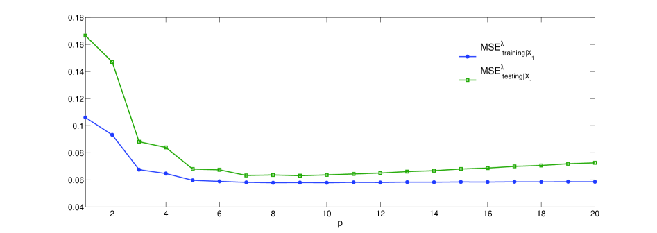
Figure 1: Conditional total training and testing errors committed by the regularized ($\lambda=0.9$) polynomial approximation of the nonlinear underlying model (3.26)-(3.27) as a function of the number of covariates $p$ or, equivalently, the degree of the polynomial approximation. The lengths of the training and testing samples are $N_{1}=20$ and $N_{2}=20$, respectively, and $\zeta,\xi\sim\mathcal{U}(-1,1)$.

Numerical illustration. Case II. Generalization performance. In this case we allow for the support of distribution for $\zeta$ used to generate the testing sample to be different from the one that defines the construction of the training sample. Indeed, we use $\xi\sim\mathcal{U}(-1,1)$ and $\zeta\sim\mathcal{U}(1,2)$ and hence the training and testing are carried out in the different intervals where $\xi$ and $\zeta$ are defined. Equivalently, in this situation the testing will be measuring the ability of the approximate model to reckon the values of the underlying model in an interval different from the one in which the training has taken place; that is why we explicitly talk in this case of generalization performance. Figure 2 shows the evolution of the conditional training and total errors for this case (for a given training covariates sample $X_{1}$ and a fixed regularization strength reported in the caption). Again, the conditional total training error is a decreasing function of $p$. As to the testing error in this case, its absolute value is much higher than in Case I and its minimum is already attained for $p=4$, that is, in this case a fourth order polynomial provides the best tradeoff in the modeling of the exponential function.

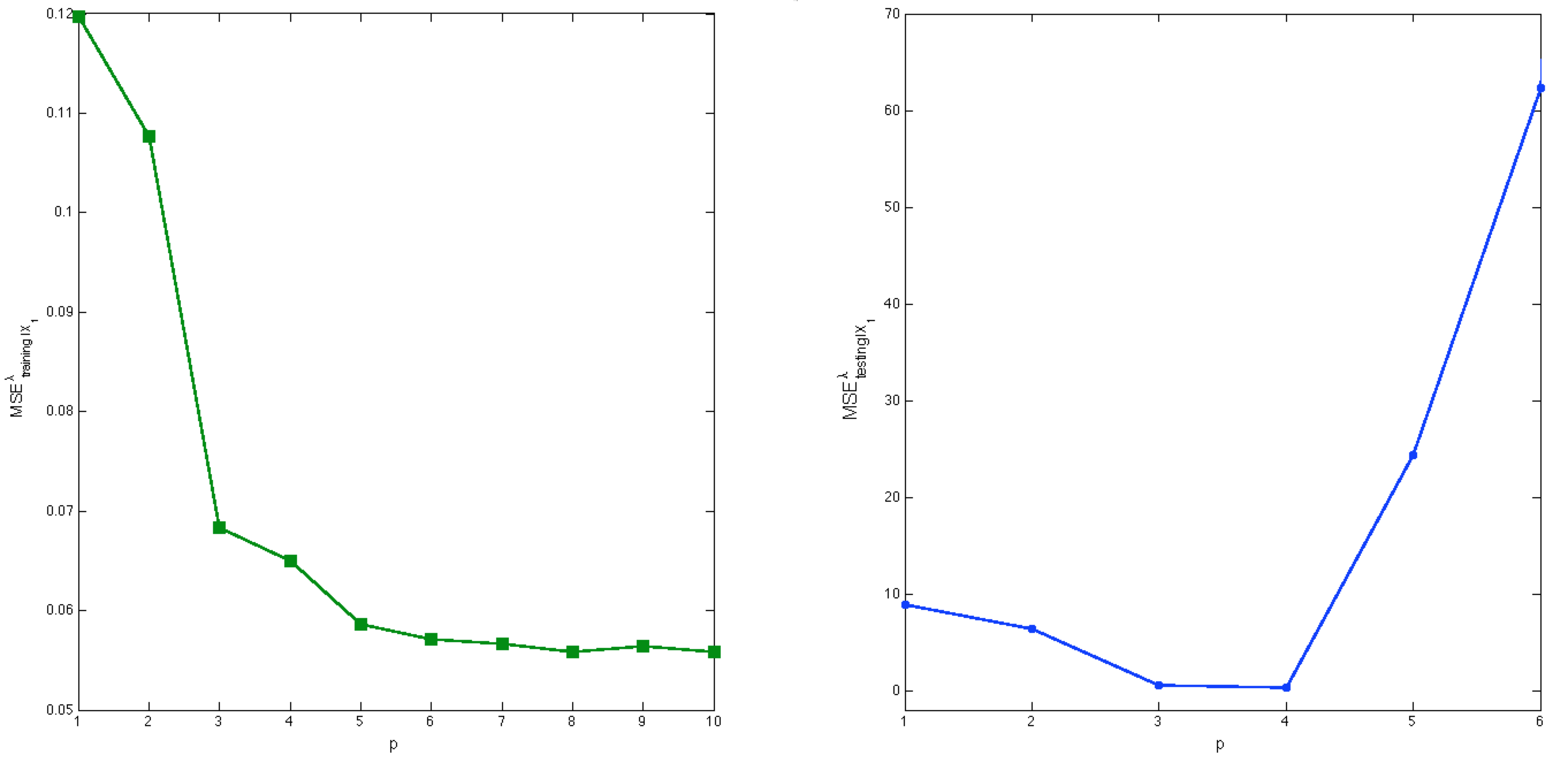
Figure 2: Conditional total training and testing errors committed by the regularized ($\lambda=1$) polynomial approximation of the nonlinear underlying model (3.26)-(3.27) as a function of the number of covariates $p$ or, equivalently, the degree of the polynomial approximation. The lengths of the training and testing samples are $N_{1}=30$ and $N_{2}=40$, respectively. The random variables $\xi\sim\mathcal{U}(-1,1)$ and $\zeta\sim\mathcal{U}(1,2)$ have been used in the dependent variables generating model.

4 Appendices

4.1 Proof of Theorem 2.3

We first notice that by definition of $R_{\lambda}$ in (2.18), namely $R_{\lambda}=(XA_{N}X^{\top}+\lambda N\mathbb{I}_{p})^{-1}$, the relation (2.9) can be rewritten as $\widehat{B}_{\lambda}=R_{\lambda}XA_{N}Y^{\top}$. In this expression we use that $Y=B_{\lambda}^{\top}X+E_{\lambda}$ and that, by the same definition of $R_{\lambda}$ in (2.18), $XAX^{\top}=R_{\lambda}^{-1}-\lambda N\mathbb{I}_{p}$. Taking both observations into account, we obtain that $\widehat{B}_{\lambda}=R_{\lambda}XA_{N}Y^{\top}=R_{\lambda}XA_{N}(X^{\top}B_{\lambda}+E_{\lambda}^{\top})=R_{\lambda}XA_{N}X^{\top}B_{\lambda}+R_{\lambda}XA_{N}E_{\lambda}^{\top}=B_{\lambda}-\lambda NR_{\lambda}B_{\lambda}+R_{\lambda}XA_{N}E_{\lambda}^{\top}$ or, equivalently,

$$\widehat{B}_{\lambda}-B_{\lambda}+\lambda NR_{\lambda}B_{\lambda}=R_{\lambda}XA_{N}E_{\lambda}^{\top}.$$ (4.1)

We now point out that the conditional homoscedasticity hypothesis on the residuals implies by Corollary 2.2 that $E_{\lambda}|X\sim{\rm MN}(M_{E_{\lambda}|X},\Sigma_{\boldsymbol{\varepsilon}|\mathbf{x}}^{\lambda},\mathbb{I}_{N})$ and hence by Theorem 2.3.10 in [Gupt 00] we have that

$$(\widehat{B}_{\lambda}-B_{\lambda}+\lambda NR_{\lambda}B_{\lambda})|X\sim{\rm MN}(R_{\lambda}XA_{N}M_{E_{\lambda}|X}^{\top},R_{\lambda}XA_{N}A_{N}^{\top}X^{\top}R_{\lambda},\Sigma_{\boldsymbol{\varepsilon}|\mathbf{x}}^{\lambda}).$$ (4.2)

Since $A_{N}A_{N}^{\top}=A_{N}$, the statement in (2.17) follows. $\blacksquare$

4.2 Proof of Lemma 2.4

Part (i). By (2.9) we have that $\widehat{B}_{\lambda}:=(XA_{N}X^{\top}+\lambda N\mathbb{I}_{p})^{-1}XA_{N}Y^{\top}$. At the same time the relation (2.26) yields $XA_{N}Y^{\top}=(XA_{N}X^{\top})\widehat{B}$, which in (2.9) gives $\widehat{B}_{\lambda}:=(XA_{N}X^{\top}+\lambda N\mathbb{I}_{p})^{-1}(XA_{N}X^{\top})\widehat{B}$. The last expression is equivalent to  (2.27), as required.

Part (ii). First, in order to establish (2.30), we notice that from the definition of $R_{\lambda}$ in (2.29), it follows that $XA_{N}X^{\top}=R_{\lambda}^{-1}-\lambda N\mathbb{I}_{p}$ and substituting this relation into (2.28) in (i) yields

$$Z_{\lambda}=R_{\lambda}XA_{N}X^{\top}=R_{\lambda}\left(R_{\lambda}^{-1}-\lambda N\mathbb{I}_{p}\right)=\mathbb{I}_{p}-\lambda NR_{\lambda},$$

as required. Second, we show that (2.31) holds. Rewriting the relation (2.28) using the definition of $R_{\lambda}$ in (2.29), we obtain that

$$Z_{\lambda}=\left((XA_{N}X^{\top})^{-1}XA_{N}X^{\top}+\lambda N(XA_{N}X^{\top})^{-1}\right)^{-1}=\left(\mathbb{I}_{p}+\lambda N(XA_{N}X^{\top})^{-1}\right)^{-1},$$

we establish that it is equivalent to (2.31), as required. $\blacksquare$

4.3 Proof of Corollary 2.6

As $\widehat{B}_{\lambda}-B=(\widehat{B}_{\lambda}-B_{\lambda})+({B}_{\lambda}-B)$, then from (2.17) in Theorem 2.3 follows that

$$(\widehat{B}_{\lambda}-B)|X\sim{\rm MN}(B_{\lambda}-B-\lambda NR_{\lambda}B_{\lambda}+R_{\lambda}XA_{N}M_{E_{\lambda}|X}^{\top},R_{\lambda}XA_{N}X^{\top}R_{\lambda},\Sigma_{\boldsymbol{\varepsilon}|\mathbf{x}}^{\lambda}).$$ (4.3)

First, notice that by (2.24) and by (2.11) we can conclude that $M_{E_{\lambda}|X}^{\top}=X^{\top}(B-B_{\lambda})$. Consequently,

$$B_{\lambda}-B-\lambda NR_{\lambda}B_{\lambda}+R_{\lambda}XA_{N}X^{\top}\left(B-B_{\lambda}\right) =B_{\lambda}-B-\lambda NR_{\lambda}B_{\lambda}+R_{\lambda}(R_{\lambda}^{-1}-\lambda N\mathbb{I}_{p})\left(B-B_{\lambda}\right)$$

$$=B_{\lambda}-B-\lambda NR_{\lambda}B_{\lambda}+B-B_{\lambda}-\lambda NR_{\lambda}B+\lambda NR_{\lambda}B_{\lambda}$$

$$=-\lambda NR_{\lambda}B,$$ (4.4)

where we used the definition of $R_{\lambda}$ in (2.18). Second, we rewrite the first scale matrix in (4.3) as follows

$$R_{\lambda}XA_{N}X^{\top}R_{\lambda} =R_{\lambda}(R_{\lambda}^{-1}-\lambda N\mathbb{I}_{p})R_{\lambda}=\left(\mathbb{I}_{p}-\lambda NR_{\lambda}\right)R_{\lambda}=Z_{\lambda}R_{\lambda}.$$ (4.5)

At the same time the second scale matrix in (4.3) in the conditions of the statement is equal to $\Sigma_{\boldsymbol{\varepsilon}}$ and hence together with (4.3) and (4.5) this yields (2.32).

Now, in order to show (2.33), we first use the definition of $Z_{\lambda}$ in (2.30) and rewrite (4.5) as

$$R_{\lambda}XA_{N}X^{\top}R_{\lambda} =Z_{\lambda}R_{\lambda}=\dfrac{1}{\lambda N}Z_{\lambda}\left(\mathbb{I}_{p}-Z_{\lambda}\right)=\dfrac{1}{\lambda N}\left(Z_{\lambda}-Z_{\lambda}^{2}\right)=\dfrac{1}{\lambda N}Z_{\lambda}\left(Z_{\lambda}^{-1}-\mathbb{I}_{p}\right)Z_{\lambda}.$$ (4.6)

As by hypothesis $XA_{N}X^{\top}$ is invertible, then by (2.31) it holds that $(XA_{N}X^{\top})^{-1}=\dfrac{1}{\lambda N}\left(Z_{\lambda}^{-1}-\mathbb{I}_{p}\right)$ and the expression (4.5) becomes

$$R_{\lambda}XA_{N}X^{\top}R_{\lambda}=Z_{\lambda}(XA_{N}X^{\top})^{-1}Z_{\lambda}.$$ (4.7)

Consequently, the relations (4.3) and (4.3) together with (4.7) guarantee (2.33), as required. $\blacksquare$

4.4 Proof of Theorem 3.1

We start by using the definition of the conditional total training error provided in (3.9). First, we define $D_{\lambda}:=\widehat{B}_{\lambda}-B_{\lambda}$ and subtract and add $B_{\lambda}$ to $\widehat{B}_{\lambda}$ in (3.9) which results in

$${\rm MSE}_{{\rm training}|X}^{\lambda} =\dfrac{1}{N}{\rm trace}\left({\rm E}_{X}\left[(Y-(\widehat{B}_{\lambda}-B_{\lambda}+B_{\lambda})^{\top}X)^{\top}(Y-(\widehat{B}_{\lambda}-B_{\lambda}+B_{\lambda})X)\right]\right)$$

$$=\dfrac{1}{N}{\rm trace}\left({\rm E}_{X}\left[(E_{\lambda}-(\widehat{B}_{\lambda}-B_{\lambda})^{\top}X)^{\top}(E_{\lambda}-(\widehat{B}_{\lambda}-B_{\lambda})^{\top}X)\right]\right)$$

$$=\dfrac{1}{N}{\rm trace}\left({\rm E}_{X}\left[(E_{\lambda}-D_{\lambda}^{\top}X)^{\top}(E_{\lambda}-D_{\lambda}^{\top}X)\right]\right)=\dfrac{1}{N}{\rm trace}({\rm E}_{X}\left[E_{\lambda}^{\top}E_{\lambda}\right])$$

$$+\dfrac{1}{N}{\rm trace}(X^{\top}{\rm E}_{X}\left[D_{\lambda}D_{\lambda}^{\top}\right]X)-\dfrac{2}{N}{\rm trace}\left(X^{\top}{\rm E}_{X}\left[D_{\lambda}E_{\lambda}\right]\right).$$ (4.8)

We now study separately the three summands in (4.4). The first one can be computed in a straightforward way. Indeed, by (i) in Lemma 2.1 we can immediately write

$$\dfrac{1}{N}{\rm trace}({\rm E}_{X}\left[E_{\lambda}^{\top}E_{\lambda}\right])={\rm trace}(\Sigma_{\boldsymbol{\varepsilon}|\mathbf{x}}^{\lambda})+\dfrac{1}{N}{\rm trace}(M_{E_{\lambda}|X}^{\top}M_{E_{\lambda}|X}).$$ (4.9)

As for the second summand, we notice first that, in the hypotheses of the theorem, the properties of the estimator $\widehat{B}_{\lambda}$ are as provided in Theorem 2.3, that is,

$$D_{\lambda}|X\sim{\rm MN}(M_{D_{\lambda}},R_{\lambda}XA_{N}X^{\top}R_{\lambda},\Sigma_{\boldsymbol{\varepsilon}|\mathbf{x}}^{\lambda}),$$ (4.10)

with

$$M_{D_{\lambda}}:=-\lambda NR_{\lambda}B_{\lambda}+R_{\lambda}XA_{N}M_{E_{\lambda}|X}^{\top}$$ (4.11)

and

$$R_{\lambda}:=(XA_{N}X^{\top}+\lambda N\mathbb{I}_{p})^{-1}.$$ (4.12)

At the same time, by Theorem 2.3.10 in [Gupt 00] (see also Lemma 6.3 in [Grig 16]) we have that $D_{\lambda}$ satisfies the following relation

$${\rm E}_{X}\left[D_{\lambda}D_{\lambda}^{\top}\right] ={\rm trace}(\Sigma_{\boldsymbol{\varepsilon}|\mathbf{x}}^{\lambda})R_{\lambda}XA_{N}X^{\top}R_{\lambda}+M_{D_{\lambda}}M_{D_{\lambda}}^{\top}.$$ (4.13)

Using this expression, we see that the second summand in (4.4) can be written as

$$\dfrac{1}{N}{\rm trace}\left(X^{\top}{\rm E}_{X}\left[D_{\lambda}D_{\lambda}^{\top}\right]X\right) =\dfrac{1}{N}{\rm trace}\left({\rm E}_{X}\left[D_{\lambda}D_{\lambda}^{\top}\right]XX^{\top}\right)$$

$$=\dfrac{1}{N}{\rm trace}\Bigg{[}\left({\rm trace}(\Sigma_{\boldsymbol{\varepsilon}|\mathbf{x}}^{\lambda})R_{\lambda}XA_{N}X^{\top}R_{\lambda}+M_{D_{\lambda}}M_{D_{\lambda}}^{\top}\right)XX^{\top}\Bigg{]}$$

$$=\dfrac{1}{N}{\rm trace}(\Sigma_{\boldsymbol{\varepsilon}|\mathbf{x}}^{\lambda})Z_{\lambda}R_{\lambda}XX^{\top}+\dfrac{1}{N}{\rm trace}(M_{D_{\lambda}}M_{D_{\lambda}}^{\top}XX^{\top}),$$ (4.14)

where

$$Z_{\lambda}:=R_{\lambda}XA_{N}X^{\top}.$$ (4.15)

Finally, we can rewrite the third summand in (4.4) by using the definition of the ridge regression matrix estimator $\widehat{B}_{\lambda}$ in (2.9) and using $R_{\lambda}$ in (4.12):

$$X^{\top}{\rm E}_{X}\left[D_{\lambda}E_{\lambda}\right]= X^{\top}{\rm E}_{X}\left[\left(\widehat{B}_{\lambda}-B_{\lambda}\right)E_{\lambda}\right]=X^{\top}{\rm E}_{X}\left[\widehat{B}_{\lambda}E_{\lambda}\right]-X^{\top}B_{\lambda}{\rm E}_{X}\left[E_{\lambda}\right]$$

$$= X^{\top}R_{\lambda}XA_{N}{\rm E}_{X}\left[Y^{\top}E_{\lambda}\right]-X^{\top}B_{\lambda}{\rm E}_{X}\left[E_{\lambda}\right]=X^{\top}R_{\lambda}X_{N}A_{N}{\rm E}_{X}\left[X^{\top}B_{\lambda}E_{\lambda}+E_{\lambda}^{\top}E_{\lambda}\right]$$

$$-X^{\top}B_{\lambda}{\rm E}_{X}\left[E_{\lambda}\right]=X^{\top}R_{\lambda}XA_{N}(X^{\top}B_{\lambda}{\rm E}_{X}\left[E_{\lambda}\right]+{\rm E}_{X}\left[E_{\lambda}^{\top}E_{\lambda}\right])-X^{\top}B_{\lambda}{\rm E}_{X}\left[E_{\lambda}\right].$$

In this expression we now use the part (i) in Lemma 2.1 and hence conclude that

$$-\dfrac{2}{N}{\rm trace}\left({\rm E}_{X}\left[X^{\top}D_{\lambda}E_{\lambda}\right]\right)= -\dfrac{2}{N}{\rm trace}\Big{(}X^{\top}R_{\lambda}XA_{N}(X^{\top}B_{\lambda}M_{E_{\lambda}|X}+{\rm trace}(\Sigma_{\boldsymbol{\varepsilon}|\mathbf{x}}^{\lambda})\mathbb{I}_{N}+M_{E_{\lambda}|X}^{\top}M_{E_{\lambda}|X})$$

$$-X^{\top}B_{\lambda}M_{E_{\lambda}|X}\Big{)}=-\dfrac{2}{N}\Big{(}{\rm trace}(\Sigma_{\boldsymbol{\varepsilon}|\mathbf{x}}^{\lambda}){\rm trace}(Z_{\lambda})$$

$$+{\rm trace}(X^{\top}R_{\lambda}XA_{N}M_{E_{\lambda}|X}^{\top}M_{E_{\lambda}|X})+{\rm trace}(\left(X^{\top}R_{\lambda}XA_{N}-\mathbb{I}_{N}\right)X^{\top}B_{\lambda}M_{E_{\lambda}|X})\Big{)}.$$ (4.16)

Using (4.9), (4.4), and (4.4) in (4.4) yields the expression (3.1). At the same time, in (3.1) the last term can be rewritten as

$$-\dfrac{2}{N}\ {\rm trace}\left((X^{\top}R_{\lambda}XA_{N}-\mathbb{I}_{N})X^{\top}B_{\lambda}M_{E_{\lambda}|X}\right) =-\dfrac{2}{N}\ {\rm trace}\left(X^{\top}(Z_{\lambda}-\mathbb{I}_{p})B_{\lambda}M_{E_{\lambda}|X}\right)$$

$$={2}\lambda{\rm trace}(X^{\top}R_{\lambda}B_{\lambda}M_{E_{\lambda}|X}),$$ (4.17)

by using (2.30). The substitution of this expression in (3.1) provides the relation (3.1). $\blacksquare$

4.5 Proof of Corollary 3.2

In order to prove (3.15), we just determine all the ingredients required for the evaluation of (3.9) in the conditions of Example A and we then show that the result follows. First, notice that by (2.25)

$$\Sigma^{\lambda}_{\boldsymbol{\varepsilon}|\mathbf{x}} =\Sigma_{\boldsymbol{\varepsilon}}$$ (4.18)

and that by (2.24)

$$M_{E_{\lambda}|X}=(B-B_{\lambda})^{\top}X.$$ (4.19)

Additionally,

$$M_{E_{\lambda}|X}^{\top}M_{E_{\lambda}|X}=X^{\top}(B-B_{\lambda})(B-B_{\lambda})^{\top}X=X^{\top}BB^{\top}X-X^{\top}BB_{\lambda}^{\top}X-X^{\top}B_{\lambda}B^{\top}X+X^{\top}B_{\lambda}B_{\lambda}^{\top}X.$$ (4.20)

We now proceed by pointing out that $M_{(\widehat{B}_{\lambda}-B_{\lambda})}=M_{\widehat{B}_{\lambda}}+B_{\lambda}$ and by using that in the conditions of Example A, the mean matrix $M_{\widehat{B}_{\lambda}}$ is given by $M_{\widehat{B}_{\lambda}}=Z_{\lambda}B$, with $Z_{\lambda}$ as in (2.19). We hence have that

$$M_{(\widehat{B}_{\lambda}-B_{\lambda})} =B_{\lambda}+Z_{\lambda}B=B_{\lambda}+(\mathbb{I}_{p}-\lambda NR_{\lambda})B=B+B_{\lambda}-\lambda NR_{\lambda}B.$$ (4.21)

Additionally, we compute

$$M_{(\widehat{B}_{\lambda}-B_{\lambda})}M_{(\widehat{B}_{\lambda}-B_{\lambda})}^{\top} =(B+B_{\lambda}-\lambda NR_{\lambda}B)(B+B_{\lambda}-\lambda NR_{\lambda}B)^{\top}=BB^{\top}-BB_{\lambda}^{\top}-B_{\lambda}B^{\top}+B_{\lambda}B_{\lambda}^{\top}$$

$$-\lambda NBB^{\top}R_{\lambda}-\lambda NR_{\lambda}BB^{\top}+\lambda NR_{\lambda}BB_{\lambda}^{\top}+\lambda NB_{\lambda}B^{\top}R_{\lambda}+\lambda^{2}N^{2}R_{\lambda}BB^{\top}R_{\lambda}.$$ (4.22)

We now substitute these expressions in the five summands that make formula (3.1) and that we analyze one. First,

$${\rm trace}(\Sigma_{\boldsymbol{\varepsilon}|\mathbf{x}}^{\lambda})={\rm trace}(\Sigma_{\boldsymbol{\varepsilon}}),$$ (4.23)

$$\dfrac{1}{N}{\rm trace}(\Sigma_{\boldsymbol{\varepsilon}|\mathbf{x}}^{\lambda}){\rm trace}\left(Z_{\lambda}(R_{\lambda}XX^{\top}-2\mathbb{I}_{p})\right)=\dfrac{1}{N}{\rm trace}(\Sigma_{\boldsymbol{\varepsilon}}){\rm trace}\left(Z_{\lambda}(R_{\lambda}XX^{\top}-2\mathbb{I}_{p})\right),$$ (4.24)

$$\dfrac{1}{N}{\rm trace}\left(M_{(\widehat{B}_{\lambda}-B_{\lambda})}M_{(\widehat{B}_{\lambda}-B_{\lambda})}^{\top}XX^{\top}\right)= \dfrac{1}{N}{\rm trace}((BB^{\top}-BB_{\lambda}^{\top}-B_{\lambda}B^{\top}+B_{\lambda}B_{\lambda}^{\top}-\lambda NBB^{\top}R_{\lambda}$$

$$-\lambda NR_{\lambda}BB^{\top}+\lambda NR_{\lambda}BB_{\lambda}^{\top}+\lambda NB_{\lambda}B^{\top}R_{\lambda}$$

$$+\lambda^{2}N^{2}R_{\lambda}BB^{\top}_{\lambda}R_{\lambda})XX^{\top}),$$ (4.25)

$$-\dfrac{2}{N}{\rm trace}((X^{\top}R_{\lambda}XA_{N} -\dfrac{1}{2}\mathbb{I}_{N})M_{E_{\lambda}|X}^{\top}M_{E_{\lambda}|X})=-\dfrac{2}{N}{\rm trace}((X^{\top}R_{\lambda}XA_{N}-\dfrac{1}{2}\mathbb{I}_{N})(X^{\top}BB^{\top}X-X^{\top}BB_{\lambda}^{\top}X$$

$$-X^{\top}B_{\lambda}B^{\top}X+X^{\top}B_{\lambda}B_{\lambda}^{\top}X))=\dfrac{1}{N}{\rm trace}((-BB^{\top}+BB_{\lambda}^{\top}+B_{\lambda}B^{\top}-B_{\lambda}B_{\lambda}^{\top}$$

$$+2\lambda NR_{\lambda}BB^{\top}-2\lambda NR_{\lambda}BB_{\lambda}^{\top}-2\lambda NR_{\lambda}B_{\lambda}B^{\top}+2\lambda NR_{\lambda}B_{\lambda}B_{\lambda}^{\top})XX^{\top}),$$ (4.26)

and finally,

$${2}\lambda{\rm trace}\left(X^{\top}R_{\lambda}B_{\lambda}M_{E_{\lambda}|X}\right)={2}\lambda{\rm trace}\left(X^{\top}R_{\lambda}B_{\lambda}(B-B_{\lambda})^{\top}X\right)={2}\lambda{\rm trace}\left((R_{\lambda}B_{\lambda}B^{\top}-R_{\lambda}B_{\lambda}B_{\lambda}^{\top})XX^{\top}\right),$$ (4.27)

respectively.

Gathering the terms (4.23)-(4.27), we obtain that

$${\rm MSE}_{{\rm training}|X}^{\lambda}= {\rm trace}(\Sigma_{\boldsymbol{\varepsilon}})+\dfrac{1}{N}{\rm trace}(\Sigma_{\boldsymbol{\varepsilon}}){\rm trace}\left(Z_{\lambda}(R_{\lambda}XX^{\top}-2\mathbb{I}_{p})\right)$$

$$+\dfrac{1}{N}{\rm trace}((BB^{\top}-BB_{\lambda}^{\top}-B_{\lambda}B^{\top}+B_{\lambda}B_{\lambda}^{\top}-\lambda NBB^{\top}R_{\lambda}-\lambda NR_{\lambda}BB^{\top}$$

$$+\lambda NB_{\lambda}B^{\top}R_{\lambda}+\lambda NR_{\lambda}BB_{\lambda}^{\top}+\lambda^{2}N^{2}R_{\lambda}BB^{\top}R_{\lambda}-BB^{\top}+BB_{\lambda}^{\top}+B_{\lambda}B^{\top}-B_{\lambda}B_{\lambda}^{\top}$$

$$+2\lambda NR_{\lambda}BB^{\top}-2\lambda NR_{\lambda}BB_{\lambda}^{\top}-2\lambda NR_{\lambda}B_{\lambda}B^{\top}+2\lambda NR_{\lambda}B_{\lambda}B_{\lambda}^{\top}+2\lambda NR_{\lambda}B_{\lambda}B^{\top}$$

$$-2\lambda NR_{\lambda}B_{\lambda}B_{\lambda}^{\top})XX^{\top})$$

$$={\rm trace}(\Sigma_{\boldsymbol{\varepsilon}})+\dfrac{1}{N}{\rm trace}(\Sigma_{\boldsymbol{\varepsilon}}){\rm trace}\left(Z_{\lambda}(R_{\lambda}XX^{\top}-2\mathbb{I}_{p})\right)+\lambda^{2}N{\rm trace}(R_{\lambda}BB^{\top}R_{\lambda}XX^{\top}),$$

which coincides with (3.15), as required. $\blacksquare$

4.6 Proof of Theorem 3.3

In order to prove (3.3), we first rewrite (3.16) as

$${\rm MSE}^{\lambda}_{{\rm testing}|X_{1}} =\dfrac{1}{N_{2}}{\rm E}_{X_{1}}\left[\left(Y_{2}-\widehat{B}_{\lambda}^{\top}X_{2}\right)^{\top}\left(Y_{2}-\widehat{B}_{\lambda}^{\top}X_{2}\right)\right]$$

$$=\dfrac{1}{N_{2}}\left[{\rm trace}\left({\rm E}_{X_{1}}\left[Y_{2}^{\top}Y_{2}\right]\right)-2\,{\rm trace}\left({\rm E}_{X_{1}}\left[Y_{2}^{\top}\widehat{B}_{\lambda}^{\top}X_{2}\right]\right)+{\rm trace}\left({\rm E}_{X_{1}}\left[X_{2}^{\top}\widehat{B}_{\lambda}\widehat{B}_{\lambda}^{\top}X_{2}\right]\right)\right].$$ (4.28)

In order to evaluate this expression, we study separately all its terms. We start with the first summand and use that the pairs of random samples $(X_{1},Y_{1})$ and $(X_{2},Y_{2})$ used for training and testing, respectively, are independent from each other. We hence rewrite the first term in (4.6) as

$$\dfrac{1}{N_{2}}{\rm trace}\left({\rm E}_{X_{1}}\left[Y_{2}^{\top}Y_{2}\right]\right)=\dfrac{1}{N_{2}}{\rm trace}\left({\rm E}\left[Y_{2}^{\top}Y_{2}\right]\right)={\rm trace}\left[\Sigma^{(2)}_{\mathbf{y}}+\boldsymbol{\mu}^{(2)}_{\mathbf{y}}\boldsymbol{\mu}_{\mathbf{y}}^{(2)\top}\right]$$ (4.29)

with

$$\Sigma^{(2)}_{\mathbf{y}} ={\rm Cov}(\mathbf{y}^{(2)},\mathbf{y}^{(2)}),$$ (4.30)

$$\boldsymbol{\mu}^{(2)}_{\mathbf{y}} ={\rm E}\left[\mathbf{y}^{(2)}\right].$$ (4.31)

For the second summand we obtain

$$-\dfrac{2}{N_{2}}{\rm trace}\left({\rm E}_{X_{1}}\left[Y_{2}^{\top}\widehat{B}_{\lambda}^{\top}X_{2}\right]\right) =-\dfrac{2}{N_{2}}{\rm trace}\left({\rm E}_{X_{1}}\left[X_{2}Y_{2}^{\top}\widehat{B}_{\lambda}^{\top}\right]\right)=-\dfrac{2}{N_{2}}{\rm trace}\left({\rm E}\left[X_{2}Y_{2}^{\top}\right]{\rm E}_{X_{1}}\left[\widehat{B}_{\lambda}^{\top}\right]\right)$$

$$=-{2}{}{\rm trace}\left(\left(\Sigma^{(2)}_{\mathbf{x}\mathbf{y}}+\boldsymbol{\mu}_{\mathbf{x}}^{(2)}\boldsymbol{\mu}_{\mathbf{y}}^{(2)\top}\right)M^{\top}_{\widehat{B}_{\lambda}}\right),$$ (4.32)

with

$$M_{\widehat{B}_{\lambda}} :=B_{\lambda}-\lambda N_{1}R_{\lambda}B_{\lambda}+R_{\lambda}X_{1}A_{N_{1}}M_{E_{\lambda}|X}^{(1)\top},$$ (4.33)

$$\Sigma^{(2)}_{\mathbf{x}\mathbf{y}} ={\rm Cov}(\mathbf{x}^{(2)},\mathbf{y}^{(2)}),$$ (4.34)

$$\boldsymbol{\mu}^{(2)}_{\mathbf{x}} ={\rm E}\left[\mathbf{x}^{(2)}\right].$$ (4.35)

In (4.6) we used the properties of the ridge regression matrix estimator $\widehat{B}_{\lambda}$ provided in Theorem 2.3. Finally, we rewrite the third term as

$$\dfrac{1}{N_{2}}{\rm trace}\left({\rm E}_{X_{1}}\left[X_{2}^{\top}\widehat{B}_{\lambda}\widehat{B}_{\lambda}^{\top}X_{2}\right]\right) =\dfrac{1}{N_{2}}{\rm trace}\left({\rm E}_{X_{1}}\left[X_{2}X_{2}^{\top}\widehat{B}_{\lambda}\widehat{B}_{\lambda}^{\top}\right]\right)=\dfrac{1}{N_{2}}{\rm trace}\left({\rm E}\left[X_{2}X_{2}^{\top}\right]{\rm E}_{X_{1}}\left[\widehat{B}_{\lambda}\widehat{B}_{\lambda}^{\top}\right]\right)$$

$$={\rm trace}\left[\left(\Sigma^{(2)}_{\mathbf{x}}+\boldsymbol{\mu}^{(2)}_{\mathbf{x}}\boldsymbol{\mu}_{\mathbf{x}}^{(2)\top}\right)\left({\rm trace}\left(\Sigma^{\lambda,(1)}_{\boldsymbol{\varepsilon}|\mathbf{x}}\right)Z_{\lambda}R_{\lambda}+M_{\widehat{B}_{\lambda}}M^{\top}_{\widehat{B}_{\lambda}}\right)\right],$$ (4.36)

with

$$\Sigma^{(2)}_{\mathbf{x}} ={\rm Cov}(\mathbf{x}^{(2)},\mathbf{x}^{(2)}),$$ (4.37)

and where $M_{\widehat{B}_{\lambda}}$ is given in (4.33). In this expression we again used Theorem 2.3 and the property (4.13). Substituting expressions (4.29)-(4.6) into (4.6) immediately yields (3.3), as required. $\blacksquare$

References

• [Gema 92] S. Geman, E. Bienenstock, and R. Doursat. “Neural Networks and the Bias/Variance Dilemma”. Neural Computation, Vol. 4, No. 1, pp. 1–58, jan 1992.
• [Grig 16] L. Grigoryeva, J. Henriques, L. Larger, and J.-P. Ortega. “Nonlinear memory capacity of parallel time-delay reservoir computers in the processing of multidimensional signals”. To appear in Neural Computation, 2016.
• [Gupt 00] A. Gupta and D. Nagar. Matrix Variate Distributions. Chapman and Hall/CRC, 2000.
• [Hami 94] J. D. Hamilton. Time series analysis. Princeton University Press, Princeton, NJ, 1994.
• [Hast 13] T. Hastie, R. Tibshirani, and J. Friedman. The Elements of Statistical Learning. Springer Verlag, second Ed., 2013.
• [Hoer 70] A. E. Hoerl and R. W. Kennard. “Ridge regression: biased estimation for nonorthogonal problems”. Technometrics, Vol. 12, No. 1, pp. 55–67, 1970.
• [Meye 00] C. Meyer. Matrix Analysis and Applied Linear Algebra Book and Solutions Manual. Society for Industrial and Applied Mathematics, 2000.
• [Tikh 43] A. N. Tikhonov. “On the stability of inverse problems”. Dokl. Akad. Nauk SSSR, Vol. 39, No. 5, pp. 195–198, 1943.
• [Tikh 63] A. N. Tikhonov. “Solution of incorrectly formulated problems and the regularization method”. Dokl. Akad. Nauk SSSR, Vol. 151, pp. 501–504, 1963.