Protecting weak measurements against systematic errors

Abstract

In this work, we consider the systematic error of quantum metrology by weak measurements under decoherence. We derive the systematic error of maximum likelihood estimation in general to the first-order approximation of a small deviation in the probability distribution, and study the robustness of standard weak measurement and postselected weak measurements against systematic errors. We show that, with a large weak value, the systematic error of a postselected weak measurement when the probe undergoes decoherence can be significantly lower than that of a standard weak measurement. This indicates another advantage of weak value amplification in improving the performance of parameter estimation. We illustrate the results by an exact numerical simulation of decoherence arising from a bosonic mode and compare it to the first-order analytical result we obtain.

I Introduction

Noise is inevitable in real quantum information protocols due to the unavoidable interactions between systems and the environment. Quantum metrology Giovannetti et al. (2004, 2011) is a quantum information protocol to enhance the sensitivity of measuring physical parameters by using quantum resources such as entanglement and squeezing. In quantum metrology, noise usually has two detrimental effects: one is reducing the estimation precision, and the other is biasing the estimate. Recently, quantum metrology in open systems has been the subject of intense study Escher et al. (2011); Demkowicz-Dobrzański et al. (2012); Tsang (2013); Kołodyński and Demkowicz-Dobrzański (2013); Alipour et al. (2014), and different kinds of quantum error correction techniques Lidar and Brun (2013) have been proposed to protect quantum metrology from noise, including quantum error correcting codes Lu et al. (2015); Arrad et al. (2014); Kessler et al. (2014); Dür et al. (2014) and dynamical decoupling Tan et al. (2013); Sekatski et al. (2015).

In a quantum measurement, the system is generally coupled to a probe, and the probe is measured to output the measurement results. When the probe is measured, it is easily disturbed by external noise since it usually must be exposed to the environment in order to be read. This noise may come from the coupling of the probe to the environment, the imperfection of the measurement techniques, etc. The noise can generally have two major effects on the measurement results: decreasing the precision and reducing the accuracy. The error correction techniques for quantum metrology reviewed above are mostly focused on preventing the loss of Fisher information, i.e., decrease in the measurement precision. In this paper we consider the systematic error instead. We study the systematic error of parameter estimation in general, and propose using weak value amplification for parameter estimation by weak measurement to suppress the systematic error caused by decoherence on the probe.

Weak value amplification is an effect in postselected weak measurements first discovered by Aharonov, Albert, and Vaidman in 1988 (AAV) Aharonov et al. (1988). They found that when the system is postselected to some appropriate state in a measurement with the pointer weakly coupled to the system, the shift of the pointer can go far beyond the eigenvalue spectrum of the system observable in the interaction Hamiltonian. Moreover, at the first-order of approximation the shift of the pointer is proportional to the small interaction parameter. Thus, the measurement result can be considered as an amplification of the interaction parameter.

Due to weak value amplification, postselected weak measurement has been proposed to amplify small physical quantities Romito et al. (2008); Brunner and Simon (2010); Feizpour et al. (2011); Li et al. (2011); Zilberberg et al. (2011); Wu and Żukowski (2012); Dressel et al. (2013); Hayat et al. (2013); Strübi and Bruder (2013); Zhou et al. (2013); Pang et al. (2014); Lyons et al. (2015); Pang and Brun (2015a). Recent state-of-the-art experimental techniques have realized the observation of weak values Ritchie et al. (1991); Pryde et al. (2005) and applied them to measuring small parameters in different physical systems Hosten and Kwiat (2008); Dixon et al. (2009); Starling et al. (2009, 2010a, 2010b); Pfeifer and Fischer (2011); Turner et al. (2011); Egan and Stone (2012); Gorodetski et al. (2012); Hofmann et al. (2012); Zhou et al. (2012); Shomroni et al. (2013); Viza et al. (2013); Xu et al. (2013); Lu et al. (2014); Magaña-Loaiza et al. (2014); Mirhosseini et al. (2014). Moreover, weak value amplification has also been found useful in quantum state tomography Shpitalnik et al. (2008); Hofmann (2010); Lundeen et al. (2011); Wu (2013); Das and Arvind (2014); Kobayashi et al. (2014); Maccone and Rusconi (2014). Reviews of the weak value technology and its applications can be found in Kofman et al. (2012); Shikano (2012); Dressel et al. (2014); Dressel (2015).

In a weak measurement, whether the system is postselected or not, noise on the probe can introduce systematic error in the measurement results. However, if the system is postselected, the interaction parameter can be amplified by the weak value while the noise on the probe is not. Thus, the weight of the probe noise in the measurement results can be significantly suppressed by the weak value. This is the core idea of how the systematic error may be decreased by the weak value amplification technique.

In this paper, we study in detail the systematic error of parameter estimation in weak measurements and the above idea of reducing the systematic error by weak value amplification. We focus on the maximum likelihood estimation (MLE) strategy in this work because it is the most efficient estimator in the asymptotic limit. We first obtain a general result for the systematic error of MLE in the first-order of a small deviation in the probability distribution. Then, we apply it to the standard weak measurement and the postselected weak measurement, and prove that the systematic error of the weak measurement can indeed be reduced by postselecting the system with a large weak value. We illustrate the result by a numerical simulation of a simple example with a qubit system, a qubit probe, and a single bosonic mode thermal bath.

It is worth mentioning that recently there has been a controversy over the precision of weak value amplification Starling et al. (2009, 2010b); Feizpour et al. (2011); Zhu et al. (2011); Dressel et al. (2013); Knee et al. (2013); Tanaka and Yamamoto (2013); Combes et al. (2014); Ferrie and Combes (2014); Jordan et al. (2014); Knee and Gauger (2014); Pang et al. (2014); Torres and Salazar-Serrano (2016); Lyons et al. (2015); Pang and Brun (2015b, a); Zhang et al. (2015). Since the Fisher information is proportional to the amount of the data and the postselection of the system discards a large portion of the measurement results, then the precision of the measurement may be lowered by the postselection. However, it was shown that the loss of Fisher information can be negligible when the initial state and the postselected state of the system are chosen properly Jordan et al. (2014); Pang et al. (2014); Pang and Brun (2015a); Viza et al. (2015); Alves et al. (2015), and that the signal-to-noise ratio (SNR) of postselected weak measurements can be made much higher than that of standard weak measurements by utilizing squeezed states for the probe Pang and Brun (2015b).

In contrast to the Fisher information, the systematic error of estimation does not scale with the amount of data. Therefore, if one can select the measurement results that deviate less from the true value of the parameter, and discard the unselected events, the accuracy of the estimate can be enhanced by proper postselection without suffering from the low postselection probability. This is how the systematic error differs from the Fisher information, and it is how we can avoid the problem of a low postselection probability that is an issue when using the Fisher information.

The structure of the paper is as follows. First, we review the weak value formalism for postselected weak measurements in Sec. II. Then, in Sec. III we study the systematic error of maximum likelihood estimation in the first-order approximation when the probability distribution deviates slightly from the ideal. The following section IV is devoted to a detailed investigation of the systematic errors of standard weak measurements and postselected weak measurements and we show the advantage of postselecting the system in protecting the measurement accuracy against decoherence. A simple qubit example is used in Sec. V to explicitly illustrate the analytical result by a numerical computation.

II Review of weak value theory

The effects of postselected weak measurements are usually characterized by weak values. (See Dressel et al. (2014) for a review of weak values.) In this section, we briefly review the weak value formalism for postselected weak measurement as a foundation for the discussion in the following sections.

In a quantum measurement, a measuring device coupled to the system is typically modeled by an interaction Hamiltonian between the system and the measuring device that can be written as

$$H_{I}=gA\otimes G\delta(t-t_{0}),$$ (1)

where $A$ and $G$ are observables of the system and the pointer, respectively, and $g$ characterizes the strength of the interaction. After the system and the measuring device are coupled, the device is then measured and outputs the measurement result.

Suppose the initial state of the system is $|\psi_{i}\rangle$, while the initial state of the pointer is $|D\rangle$, then the system and the pointer are coupled by the interaction, and evolve to an entangled state

$$|\Phi\rangle=\exp(-\mathrm{i}gA\otimes G)|\psi_{i}\rangle|D\rangle.$$ (2)

The evolved state $|\Phi\rangle$ can be written as

$$|\Phi\rangle=\sum_{k}c_{k}|a_{k}\rangle\exp(-\mathrm{i}ga_{k}G)|D\rangle,$$ (3)

where $a_{k},\,|a_{k}\rangle$ are eigenvalues and eigenstates of $A$, and $c_{k}$ are the expansion coefficients of $|\psi_{i}\rangle$ in the basis $\{|a_{k}\rangle\}$.

In a projective quantum measurement, the coupling between the system and the pointer is usually sufficiently strong, so that the overlaps between different $\exp(-\mathrm{i}ga_{k}G)|D\rangle$ are very small. In this case, the $\exp(-\mathrm{i}ga_{k}G)|D\rangle$ can be distinguished with a low error probability, and the measurement to distinguish different $\exp(-\mathrm{i}ga_{k}G)|D\rangle$ will collapse the system to a state close to an eigenstate of $A$. This is what the theory of standard projective quantum measurement tells us: the results of a projective quantum measurement are the eigenvalues of the observable that is measured, and the system will collapse to an eigenstate of that observable. On the contrary, in a weak measurement, the coupling between the system and the pointer is usually very weak, and different $\exp(-\mathrm{i}ga_{k}G)|D\rangle$ may substantially overlap.

The invention of AAV in weak measurements is to introduce postselection to the system which is weakly coupled to the measuring device. This small change gives dramatically different results from the standard projective quantum measurements. If the system is postselected to the state $|\psi_{f}\rangle$ after it is coupled to the measuring device, then the measuring device collapses to

$$|D_{f}\rangle=\langle\psi_{f}|\exp(-\mathrm{i}gA\otimes G)|\psi_{i}\rangle|D\rangle.$$ (4)

In a weak measurement $g$ is usually very small therefore $|D_{f}\rangle$ can be approximated by

$$|D_{f}\rangle \approx\langle\psi_{f}|(1-\mathrm{i}gA\otimes G)|\psi_{i}\rangle|D\rangle$$ (5)

$$=\langle\psi_{f}|\psi_{i}\rangle(1-\mathrm{i}gA_{w}G)|D\rangle,$$

where $A_{w}$ is defined as a weak value,

$$A_{w}=\frac{\langle\psi_{f}|A|\psi_{i}\rangle}{\langle\psi_{f}|\psi_{i}\rangle}.$$ (6)

If $gA_{w}\ll 1$ is satisfied, $|D_{f}\rangle$ can be rewritten as

$$|D_{f}\rangle\approx\exp(-\mathrm{i}gA_{w}G)|D\rangle.$$ (7)

Therefore, when the system is postselected after the weak interaction with the measuring device, the measuring device is approximately rotated by $\exp(-\mathrm{i}gA_{w}G)$. This is in sharp contrast to the standard projective measurement, because $A_{w}$ can be much larger than $1$ when $|\langle\psi_{f}|\psi_{i}\rangle|\ll 1$, and the rotation of the measuring device can be much larger than the eigenvalues of $A$ in the postselected case.

Note that $A_{w}$ can be complex, and in this case $\exp(-\mathrm{i}gA_{w}G)$ is not just a simple translation operator. In fact, it can be decomposed as the product of a translation operator (corresponding to the real part of $A_{w}$) and a state reduction operator (corresponding to the imaginary part of $A_{w}$). Jozsa gave a very detailed study of complex weak values in Ref. Jozsa (2007) and analyzed the role of the real and imaginary parts of the weak value. He showed that, if the pointer observable $G$ is the momentum $\hat{p}$, then the shifts in the average position and momentum of the pointer are, respectively,

$$\langle\Delta\hat{q}\rangle= g\mathrm{Re}A_{w}+gm\mathrm{Im}A_{w}\frac{\mathrm{d}}{\mathrm{d}t}\mathrm{Var}(\hat{q}),$$ (8)

$$\langle\Delta\hat{p}\rangle= 2g\mathrm{Im}A_{w}\mathrm{Var}(\hat{p}),$$

where $\hat{q}$ and $\hat{p}$ are the position and momentum operators of the pointer, and $m$ is the mass of the pointer.

That result can be cast in a more general form. Suppose we measure an observable $\hat{M}$ on the pointer after postselecting the system. The average shift of the pointer is

$$\langle\Delta\hat{M}\rangle_{f}=\frac{\langle D_{f}|\hat{M}|D_{f}\rangle}{\langle D_{f}|D_{f}\rangle}-\langle\hat{M}\rangle_{|D\rangle}.$$ (9)

From Eq. (5), one can get

$$\langle D_{f}|\hat{M}|D_{f}\rangle\approx |\langle\psi_{f}|\psi_{i}\rangle|^{2}[\langle\hat{M}\rangle_{|D\rangle}+\mathrm{i}g\mathrm{Re}A_{w}\langle[G,\hat{M}]\rangle_{|D\rangle}$$ (10)

$$+g\mathrm{Im}A_{w}\langle\{G,\hat{M}\}\rangle_{|D\rangle}],$$

$$\langle D_{f}|D_{f}\rangle\approx |\langle\psi_{f}|\psi_{i}\rangle|^{2}[1+2g\mathrm{Im}A_{w}\langle G\rangle_{|D\rangle}],$$

thus,

$$\langle\Delta\hat{M}\rangle_{f}\approx g\mathrm{Im}A_{w}(\langle\{G,\hat{M}\}\rangle_{|D\rangle}-2\langle G\rangle_{|D\rangle}\langle\hat{M}\rangle_{|D\rangle})$$ (11)

$$+\mathrm{i}g\mathrm{Re}A_{w}\langle[G,\hat{M}]\rangle_{|D\rangle},$$

which is similar to the result in Dressel and Jordan (2012). Note that if we plug $G=\hat{p}$ and $\hat{M}=\hat{q},\,\hat{p}$ into (11), the result in (8) can be immediately recovered.

Eqs. (8) and (11) imply that the shift of the pointer is roughly proportional to the weak value $A_{w}$ when $g\ll 1$. Since $A_{w}$ can be much larger than $1$ when $\langle\psi_{f}|\psi_{i}\rangle\ll 1$, the shift of the pointer can be treated as an amplification of $g$ by the weak value $A_{w}$. This is the origin of the amplification effect in postselected weak measurements. This amplification effect has been widely used in experiments to measure small parameters, as reviewed in the introduction.

III Systematic error of maximum likelihood estimation

In maximal likelihood estimation (MLE), suppose we want to estimate an unknown parameter $g$ from a $g$-dependent probability distribution $P_{g}:\,p_{k}(g),\,k=1,\cdots,d.$ However, due to the interaction with a noisy environment, the real probability distribution observed in experiments is $P_{g_{0}}^{{\rm expt}}:\,p_{k}^{{\rm expt}}(g),\,k=1,\cdots,d$, which slightly deviates from $p_{k}(g)$. Then, the estimate of $g$ will generally deviate from the true value $g_{0}$, i.e., a systematic error may occur in this case. In this section, we derive a general first-order solution to the systematic error for such a noisy MLE.

Suppose we observe the result $k$ a total of $N_{k}$ times in an experiment, and the measurement results are uncorrelated. The spirit of MLE is finding the most likely $g$ (the parameter to estimate) conditioned on the observation results as the estimate for $g$. In a mathematical language, it means to maximize the following likelihood function over $g$: $\mathcal{L}=\prod_{k}p_{k}^{N_{k}}(g)$, or alternatively its logarithm $\ln\mathcal{L}=\sum_{k}N_{k}\ln p_{k}(g)$.

When the total number of measurement results $N=\sum_{k}N_{k}$ is very large, $N_{k}\approx Np_{k}^{{\rm expt}}(g_{0})$ in average, so the MLE leads to the following equation with respect to $g$:

$$\partial_{g}\ln\mathcal{L}\approx N\sum_{k}p_{k}^{{\rm expt}}(g_{0})\frac{\partial_{g}p_{k}(g)}{p_{k}(g)}=0.$$ (12)

This equation usually produces multiple solutions for $g$, and we need to find the one that has the largest likelihood. It should be noted that the derivative with respect to $g$ is always performed on $p_{k}(g)$ in Eq. (12), because $p_{k}^{{\rm expt}}(g_{0})$ is the average frequency that the $k$-th result will be observed in an experiment and $g_{0}$ is the true value of $g$ (which is a constant).

When $p_{k}^{{\rm expt}}(g)=p_{k}(g),\,k=1,\cdots,d,$ it is obvious that $g=g_{0}$ is the solution to (12) since $\sum_{k}p_{k}(g)=1$, which implies that the MLE is an unbiased estimation strategy in this case. However if $p_{k}^{{\rm expt}}(g)\neq p_{k}(g),$ then generally $g\neq g_{0}$, which leads to a systematic error. (Note that the systematic error cannot be eliminated by repetition of the measurements.) If we write $g=g_{0}+\delta g$, then the question is how large $\delta g$ is in terms of the deviation of $p_{k}(g)$ from $p_{k}^{{\rm expt}}(g)$.

Suppose $p_{k}^{{\rm expt}}(g)=p_{k}(g)+q_{k}(g),\,k=1,\cdots,d,$ where $|q_{k}(g)|\ll 1$, and $\sum_{k}q_{k}(g)=0$. In this case, Eq. (12) becomes

$$\sum_{k}(p_{k}(g_{0})+q_{k}(g_{0}))\frac{\partial_{g}p_{k}(g)}{p_{k}(g)}=0.$$ (13)

If we expand $\frac{\partial_{g}p_{k}(g)}{p_{k}(g)}$ to the first-order of $\delta g$, then

$$\sum_{k}(p_{k}(g_{0})+q_{k}(g_{0}))\bigg{(}\left.\frac{\partial_{g}p_{k}(g)}{p_{k}(g)}\right|_{g=g_{0}}$$ (14)

$$+\delta g\left.\frac{p_{k}(g)\partial_{g}^{2}p_{k}(g)-(\partial_{g}p_{k}(g))^{2}}{p_{k}^{2}(g_{0})}\right|_{g=g_{0}}\bigg{)}=0.$$

Up to the first-order of $|q_{k}(g)|$, we get

$$\delta g\approx\frac{\partial_{g}\mathcal{C}(Q_{g_{0}}||P_{g})|_{g=g_{0}}}{\mathcal{F}(P_{g_{0}})},$$ (15)

where $\mathcal{C}(Q_{g_{0}}||P_{g})$ is

$$\mathcal{C}(Q_{g_{0}}||P_{g})=\sum_{k}q_{k}(g_{0})\ln p_{k}(g),$$ (16)

and $\mathcal{F}(P_{g})$ is the Fisher information of the probability distribution $P_{g}$ at $g=g_{0}$,

$$\mathcal{F}(P_{g_{0}})=\sum_{k}\left.\frac{(\partial_{g}p_{k}(g))^{2}}{p_{k}(g)}\right|_{g=g_{0}}.$$ (17)

Since $q_{k}(g)=p_{k}^{{\rm expt}}(g)-p_{k}(g)$ and the derivative is with respect to $g$ only, $\partial_{g}\mathcal{C}(Q_{g_{0}}||P_{g})$ can be written as

$$\partial_{g}\mathcal{C}(Q_{g_{0}}||P_{g})$$ (18)

$$=\partial_{g}\sum_{k}p_{k}^{{\rm expt}}(g_{0})(\ln p_{k}(g)-\ln p_{k}^{{\rm expt}}(g_{0}))$$

$$-\partial_{g}\sum_{k}p_{k}(g_{0})\ln p_{k}(g).$$

At $g=g_{0}$,

$$\sum_{k}p_{k}(g_{0})\partial_{g}\ln p_{k}(g)|_{g=g_{0}}=0,$$ (19)

so only the first term on the right side of Eq. (18) is nonzero. Thus,

$$\partial_{g}\mathcal{C}(Q_{g_{0}}||P_{g})|_{g=g_{0}}=-\partial_{g}\mathcal{D}(P_{g_{0}}^{{\rm expt}}||P_{g})|_{g=g_{0}},$$ (20)

where $\mathcal{D}(P_{g_{0}}^{{\rm expt}}||P_{g})$ is the relative entropy between $P_{g_{0}}^{{\rm expt}}$ and $P_{g}$,

$$\mathcal{D}(P_{g_{0}}^{{\rm expt}}||P_{g})=\sum_{k}p_{k}^{{\rm expt}}(g_{0})\ln\frac{p_{k}^{{\rm expt}}(g_{0})}{p_{k}(g)}.$$ (21)

Therefore, the first-order systematic error $\delta g$ given in (15) can be finally written as

$$\delta g=-\frac{\partial_{g}\mathcal{D}(P_{g_{0}}^{{\rm expt}}||P_{g})|_{g=g_{0}}}{\mathcal{F}(P_{g_{0}})},$$ (22)

the ratio of the derivative of relative entropy to the Fisher information.

Before concluding this section, we want to mention a substantial difference between the systematic error and the variance of an estimator. The Cramér-Rao bound Cramér (1946) tells us that

$$\langle\delta g^{2}\rangle\geq\frac{1}{N\mathcal{F}_{g}}+\langle\delta g\rangle^{2}.$$ (23)

The first term is the inverse of the Fisher information, which is the lower bound of the variance of the estimator. It can be seen that the variance scales as $N^{-1}$, the standard quantum limit. In contrast, the second term, i.e., the systematic error, does not depend on $N$, which implies it cannot be changed by the number of measurements.

This observation has two important implications. The first one is that systematic errors cannot be reduced simply by increasing the number of measurements, as random noise is usually treated, so when $N\rightarrow\infty$, the random errors will approach zero but the systematic errors will remain finite, thus it calls for new methods to overcome the systematic errors. The other is that if weak value amplification can reduce the systematic error (as we will show later), the low postselection probability will not affect it, since the systematic error is not proportional to the size of the data. This is the foundation of weak value amplification in suppressing systematic errors in weak measurements.

IV Weak measurements with decoherence

In this section, we study the systematic error of weak measurements with or without postselection in the presence of decoherence and show the effect of large weak values in suppressing the systematic errors.

We first give some general analysis about the systematic error in a standard or a postselected weak measurement. From Eq. (22), we can see that the systematic error of the MLE is the reciprocal of the Fisher information. Since the Fisher information can be amplified by the order of $|A_{w}|^{2}$ when the system is postselected, and it cannot be reduced by the postselection probability since it is not dependent on the size of data according to (22), then a large weak value may reduce the systematic error. Note that $\partial_{g}\mathcal{D}(P_{g_{0}}^{{\rm expt}}||P_{g})$ may also be amplified by the weak value because the probability distribution of the measurement results on the probe is approximately shifted by $gA_{w}$ according to (11), but the order of the amplification factor is $|A_{w}|$. So the net effect of weak value amplification is to reduce the systematic error by the order of $|A_{w}|$.

Below, we study the systematic error of weak measurements and the effect of weak value amplification on reducing it in detail. Throughout this paper, we let $\hbar=1$ for simplicity.

When the pointer undergoes decoherence, a typical interaction Hamiltonian is

$$H_{I}=gA\otimes G\delta(t-t_{0})+\epsilon_{D}H_{DE},\,g,\epsilon_{D}\ll 1,$$ (24)

where the subscripts $S$, $D$, $E$ represent the system, the probe and the environment respectively. For simplicity, we assume that $g,\epsilon_{D}\ll 1$ and that $g^{2}\ll\epsilon_{D}$ so that the second order of $g$ can be neglected. Suppose the initial states of the system and the probe are $\rho_{S},\,\rho_{D},$ and the initial state of the environment is $\rho_{E}$. Then, after time $t$, the joint state of the system, probe and environment is

$$\rho_{SDE}^{{\rm expt}}(t)=\exp(-\mathrm{i}H_{I}t)\rho_{S}\otimes\rho_{D}\otimes\rho_{E}\exp(\mathrm{i}H_{I}t).$$ (25)

When the interaction time is very short, i.e., $t\ll 1,$ we have

$$\rho_{SDE}^{{\rm expt}}(t)\approx \rho_{S}\otimes\rho_{D}\otimes\rho_{E}-\mathrm{i}[gA\otimes G$$ (26)

$$+\epsilon_{D}tH_{DE},\,\rho_{S}\otimes\rho_{D}\otimes\rho_{E}].$$

If there is no decoherence on the probe, $\epsilon_{D}=0$, the joint state of the system, probe and environment can be reduced to

$$\rho_{SDE}(t)=(\rho_{S}\otimes\rho_{D}-\mathrm{i}g[A\otimes G,\,\rho_{S}\otimes\rho_{D}])\otimes\rho_{E}.$$ (27)

So, the joint state $\rho_{SDE}^{\exp}(t)$ in the presence of decoherence can be rewritten as

$$\rho_{SDE}^{{\rm expt}}(t)=\rho_{SDE}(t)-\mathrm{i}t[\epsilon_{D}H_{DE},\,\rho_{S}\otimes\rho_{D}\otimes\rho_{E}].$$ (28)

IV.1 Standard weak measurement

When there is no postselection on the system in the weak measurement, the post-interaction pointer state in the absence of decoherence is

$$\rho_{D}(t) \approx\rho_{D}-\mathrm{i}g\mathrm{Tr}_{S}[A\otimes G,\,\rho_{S}\otimes\rho_{D}]$$ (29)

$$\approx\rho_{D}-\mathrm{i}g\langle A\rangle_{i}[G,\,\rho_{D}],$$

where

$$\langle A\rangle_{i}=\mathrm{Tr}_{S}(A\rho_{S}).$$ (30)

And the post-interaction probe state in the presence of decoherence is

$$\rho_{D}^{{\rm expt}}(t) \approx\rho_{D}(t)-\mathrm{i}t\mathrm{Tr}_{SE}[\epsilon_{D}H_{DE},\,\rho_{S}\otimes\rho_{D}\otimes\rho_{E}]$$ (31)

$$=\rho_{D}(t)-\mathrm{i}t\epsilon_{D}[H_{D}^{\prime},\,\rho_{D}],$$

where

$$H_{D}^{\prime}=\mathrm{Tr}_{E}(H_{DE}\rho_{E}).$$ (32)

Now, if we measure an orthonormal basis $\{|k\rangle\}$ on the post-interaction probe state, the probability distribution in the decoherence-free case is

$$p_{k}(g)=\langle k|\rho_{D}|k\rangle-\mathrm{i}g\langle A\rangle_{i}\langle k|[G,\rho_{D}]|k\rangle,$$ (33)

and the probability distribution for the case with decoherence is

$$p_{k}^{{\rm expt}}(g)=p_{k}(g)+q_{k}(g),$$ (34)

where

$$q_{k}(g)=-\mathrm{i}\epsilon_{D}t\langle k|[H_{D}^{\prime},\rho_{D}]|k\rangle.$$ (35)

Then, since $g\ll 1,$ we have

$$\partial_{g}\mathcal{D}(P_{g_{0}}^{{\rm expt}}||P_{g})|_{g=g_{0}} \approx\epsilon_{D}t\langle A\rangle_{i}\times$$ (36)

$$\sum_{k}\frac{\langle k|[H_{D}^{\prime},\rho_{D}]|k\rangle\langle k|[G,\rho_{D}]|k\rangle}{\langle k|\rho_{D}|k\rangle},$$

$$\mathcal{F}(P_{g_{0}}) \approx\langle A\rangle_{i}^{2}\sum_{k}\frac{|\langle k|[G,\rho_{D}]|k\rangle|^{2}}{\langle k|\rho_{D}|k\rangle}.$$

If we define the following weak values for $G$ and $H_{D}^{\prime}$

$$G_{w}^{(k)}=\frac{\langle k|G\rho_{D}|k\rangle}{\langle k|\rho_{D}|k\rangle},\,H_{Dw}^{\prime(k)}=\frac{\langle k|H_{D}^{\prime}\rho_{D}|k\rangle}{\langle k|\rho_{D}|k\rangle},$$ (37)

then (36) can be simplified to

$$\partial_{g}\mathcal{D}(P_{g_{0}}^{{\rm expt}}||P_{g})|_{g=g_{0}} \approx-4\epsilon_{D}t\langle A\rangle_{i}\times$$ (38)

$$\sum_{k}\langle k|\rho_{D}|k\rangle\mathrm{Im}H_{Dw}^{\prime(k)}\mathrm{Im}G_{w}^{(k)},$$

$$\mathcal{F}(P_{g_{0}}) \approx 4\langle A\rangle_{i}^{2}\sum_{k}\langle k|\rho_{D}|k\rangle\mathrm{Im}^{2}G_{w}^{(k)}.$$

Therefore, according to Eq. (22), the systematic error $\delta g_{n}$ of the standard weak measurement which has no postselection on the system is approximately

$$\delta g_{n}\approx\frac{\epsilon_{D}t{\displaystyle\sum_{k}\langle k|\rho_{D}|k\rangle\mathrm{Im}H_{Dw}^{\prime(k)}\mathrm{Im}G_{w}^{(k)}}}{\langle A\rangle_{i}{\displaystyle\sum_{k}\langle k|\rho_{D}|k\rangle\mathrm{Im}^{2}G_{w}^{(k)}}}.$$ (39)

From the above result, we can see that generally the initial state of the system should not be chosen such that $\langle A\rangle_{i}\ll 1$, otherwise, the Fisher information of the measurement in Eq. (36) will be very small, implying a bad estimation precision, and the systematic error in Eq. (39) will be very large, implying a large deviation of the measurement result from the true value of the parameter.

IV.2 Postselected weak measurement

In a postselected weak measurement, the system is postselected to some specific state $|\psi_{f}\rangle$ after it is coupled to the probe. So the pointer state after the postselection of the system in the absence of decoherence is

$$\rho_{D}(t)\approx \langle\psi_{f}|\rho_{S}|\psi_{f}\rangle\rho_{D}-\mathrm{i}g\langle\psi_{f}|[A\otimes G,\rho_{S}\otimes\rho_{D}]|\psi_{f}\rangle$$ (40)

$$= \langle\psi_{f}|\rho_{S}|\psi_{f}\rangle(\rho_{D}-\mathrm{i}g\mathrm{Re}A_{w}{}[G,\,\rho_{D}]$$

$$+g\mathrm{Im}A_{w}\{G,\,\rho_{D}\}).$$

In the presence of decoherence on the probe, the post-interaction probe state formed by tracing out the environment is

$$\rho_{D}^{{\rm expt}}(t)\approx \rho_{D}(t)-\mathrm{i}\epsilon_{D}t\langle\psi_{f}|\rho_{S}|\psi_{f}\rangle[H_{D}^{\prime},\rho_{D}],$$ (41)

$$\propto \rho_{D}-\mathrm{i}g\mathrm{Re}A_{w}{}[G,\,\rho_{D}]$$

$$+g\mathrm{Im}A_{w}\{G,\,\rho_{D}\}-\mathrm{i}\epsilon_{D}t[H_{D}^{\prime},\rho_{D}],$$

where $H_{D}^{\prime}$ is defined in Eq. (32).

Now, if we measure along an orthonormal basis $\{|k\rangle\}$ on the post-interaction pointer state, the probability distribution of the measurement results in the decoherence-free case is

$$p_{k}(g)= \langle k|\rho_{D}|k\rangle-\mathrm{i}g\mathrm{Re}A_{w}\langle k|[G,\,\rho_{D}]|k\rangle$$ (42)

$$+g\mathrm{Im}A_{w}\langle k|\{G,\,\rho_{D}\}|k\rangle.$$

If we define the following weak value for $G$,

$$G_{w}^{(k)}=\frac{\langle k|G\rho_{D}|k\rangle}{\langle k|\rho_{D}|k\rangle},$$ (43)

then,

$$p_{k}(g) =\langle k|\rho_{D}|k\rangle[1+2g(\mathrm{Re}A_{w}\mathrm{Im}G_{w}^{(k)}+\mathrm{Im}A_{w}\mathrm{Re}G_{w}^{(k)})]$$ (44)

$$=\langle k|\rho_{D}|k\rangle[1+2g\mathrm{Im}(A_{w}G_{w}^{(k)})].$$

Also, the probability distribution of the measurement results in the presence of decoherence is

$$p_{k}^{{\rm expt}}(g)=p_{k}(g)+q_{k}(g),$$ (45)

and

$$q_{k}(g)=2\langle k|\rho_{D}|k\rangle t\epsilon_{D}\mathrm{Im}H_{Dw}^{\prime(k)},$$ (46)

where $H_{Dw}^{\prime(k)}$ is defined as

$$H_{Dw}^{\prime(k)}=\frac{\langle k|H_{D}^{\prime}\rho_{D}|k\rangle}{\langle k|\rho_{D}|k\rangle}.$$ (47)

In the weak interaction limit $g\ll 1$, we can see that

$$\partial_{g}\mathcal{D}(P_{g_{0}}^{{\rm expt}}||P_{g})|_{g=g_{0}} \approx 4t\sum_{k}\langle k|\rho_{D}|k\rangle\epsilon_{D}\mathrm{Im}H_{Dw}^{\prime(k)}\mathrm{Im}(A_{w}G_{w}^{(k)})$$ (48)

$$\mathcal{F}(P_{g_{0}}) \approx 4\sum_{k}\langle k|\rho_{D}|k\rangle\mathrm{Im}^{2}(A_{w}G_{w}^{(k)}).$$

Therefore, the systematic error $\delta g_{p}$ when the system is postselected to $|\psi_{f}\rangle$ is

$$\delta g_{p}\approx\frac{{\displaystyle\epsilon_{D}t\sum_{k}\langle k|\rho_{D}|k\rangle\mathrm{Im}H_{Dw}^{\prime(k)}\mathrm{Im}(A_{w}G_{w}^{(k)})}}{{\displaystyle\sum_{k}\langle k|\rho_{D}|k\rangle\mathrm{Im}^{2}(A_{w}G_{w}^{(k)})}}.$$ (49)

When the postselection probability $\langle\psi_{f}|\rho_{S}|\psi_{f}\rangle\ll 1,$ the weak value $A_{w}$ of system observable $A$, is of order $\langle\psi_{f}|\rho_{S}|\psi_{f}\rangle^{-\frac{1}{2}}$, which can be very large. And $\delta g_{p}$ is proportional to the inverse of the system weak value $A_{w}$. (Note that there is no average over $A_{w}$.) Therefore, this implies that the systematic error due to the decoherence can be suppressed by a large weak value, when the system is postselected to a state that is almost orthogonal to its initial state.

A notable point here is that if we know $H_{D}^{\prime}$ exactly, there may be an even simpler (and perhaps more efficient) way to decrease the systematic error. That is, we can simply choose proper initial state and measurement basis for the probe such that $\partial_{g}\mathcal{D}(P_{g_{0}}^{{\rm expt}}||P_{g})$ [i.e., the numerator of Eq. (39)] is close to zero, in which case the systematic error becomes extremely small (it is generally still nonzero because only the first-order terms of $g$ and $\epsilon_{D}$ are considered in the above results). For example, provided that we have detailed knowledge about $H_{D}^{\prime}$, we can choose a basis $\{|k\rangle\}$ for the measurement on the probe such that all $H_{Dw}^{\prime(k)}$ are real, thus $\mathrm{Im}H_{Dw}^{\prime(k)}=0$ for all $k$, and $\delta g_{n}$ (and $\delta g_{p}$) would be approximately zero. This is a simpler way to suppress the systematic error, and postselection of the system is not so necessary in this case.

However, in practice, the interaction between the probe and the environment can be very complex, and one generally does not have complete information about the decoherence, so it is usually not practical to decrease the systematic error in this simpler way. In contrast, the method proposed above, which is based on the weak value amplification, only requires a large weak value $A_{w}$, regardless of the details of the decoherence, so this method provides a universal approach for reducing the systematic error in weak measurements.

V Numerical example

To illustrate the results derived in the previous section, we consider a simple qubit dephasing model and use a numerical computation to showcase the effects of postselection in the estimation of the system and probe coupling while varying different parameters of the model.

Suppose the total Hamiltonian for the system, probe, and environment is

$$H=g\sigma_{S}^{z}\otimes\sigma_{D}^{z}\delta(t-t_{0})+\epsilon_{D}\sigma_{D}^{y}\otimes b^{\dagger}b,$$ (50)

where $g,\,\epsilon_{D}\ll 1$ and the environment is assumed to have a single bosonic mode $b$. In Eq. (50), we only considered the coupling between the $y$-components of the probe qubit and the environment for simplicity. Generally, there can also be coupling between $x$, and $z$-components of the qubit and the environment.

Suppose the system and the probe are initially in states $|\psi_{i}\rangle$ and $|D\rangle$, and that the environment is initially in the thermal equilibrium state $\rho_{E}$,

$$\rho_{E}=\frac{1}{Z}\exp(-\beta b^{\dagger}b),\,\beta=\frac{\omega}{kT},$$ (51)

where $\omega$ is the frequency of the single mode oscillator of the environment, $k$ is the Boltzmann constant, and $T$ is the temperature of the environment. The partition function $Z$ is given by

$$Z=\mathrm{Tr}\exp(-\beta b^{\dagger}b)=\frac{1}{1-\exp(-\beta)}.$$ (52)

After a short time $t$, the joint state of the system and probe evolves to

$$\rho_{SD}=\frac{1}{Z}\sum_{n}\mathrm{e}^{-\mathrm{i}\beta n}|\Phi_{f}^{(n)}\rangle\langle\Phi_{f}^{(n)}|,$$ (53)

where $|\Phi_{f}^{(n)}\rangle$ is

$$|\Phi_{f}^{(n)}\rangle=\exp[-\mathrm{i}(g\sigma_{S}^{z}\otimes\sigma_{D}^{z}+tn\epsilon_{D}\sigma_{D}^{y})]|\psi_{i}\rangle|D\rangle.$$ (54)

In our numerical simulation, we chose $|\psi_{i}\rangle=|+\rangle$ and $|D\rangle=|+\rangle$ as the initial states for the system and the probe, respectively. The postselected state of the system is

$$|\psi_{f}\rangle=\exp\left(-\mathrm{i}\delta\sigma_{S}^{y}\right)|-\rangle,\,\delta\ll 1.$$ (55)

Hence, the weak value of $\sigma_{z}$ is

$$(\sigma_{S}^{z})_{w}=\frac{\langle\psi_{f}|\sigma_{S}^{z}|\psi_{i}\rangle}{\langle\psi_{f}|\psi_{i}\rangle}=\cot\delta,$$ (56)

which is approximately $1/\delta$ when $\delta\ll 1$. The measurement basis that we choose on the probe is

$$|k^{\prime}\rangle=\mathrm{e}^{-\mathrm{i}\theta\sigma^{x}}|k\rangle,\;k=0,\,1,$$ (57)

where $\theta$ is a parameter to adjust.

Below we plot the numerical results for this example varying the values of the different parameters of interest. Unless otherwise noted, we fix $\beta=1.0,\,\theta=\frac{\pi}{8},\,\delta=1.0\times 10^{-3},\,g=1.0\times 10^{-5}$, and $\epsilon_{D}^{i}=1.0\times 10^{-5}$. In all plots, we show the ratio of the systematic uncertainty with and without postselection on the system, $\frac{\delta g_{p}}{\delta g_{n}}$.

Fig. 1 shows the ratio $\frac{\delta g_{p}}{\delta g_{n}}$ with different choices of the postselected state with varying $\delta$.

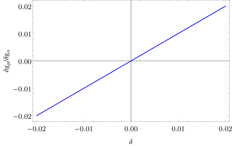
Figure 1: Ratio between the systematic error with and without postselection of the system for postselected states with varying $\delta$.

As we can see in Fig. 1, when comparing the systematic error of the estimation with and without postselection, we find that the postselection will suppress the systematic error of estimation by the order of $\delta$. This is expected because we see from Eqs. (39) and (49) that when all the parameters but $\delta$ are kept fixed, the systematic error without postselection does not depend on $\delta$, while for the postselection case, the systematic error is approximately proportional to $\delta$ when $\left|\delta\right|\ll 1$.

Fig. 2 shows the ratio $\frac{\delta g_{p}}{\delta g_{n}}$ for a range of values of the interaction parameter $g$. The figure shows that the ratio varies approximately parabolically with $g$. This is due to the second order terms of $g$ which are neglected in the weak value formalism and our results. In spite of this, the figure still shows that the suppression ratio of the systematic error has the order $10^{-3}$, approximately the inverse of the weak value $1/\delta$, which matches the theoretical results we obtained.

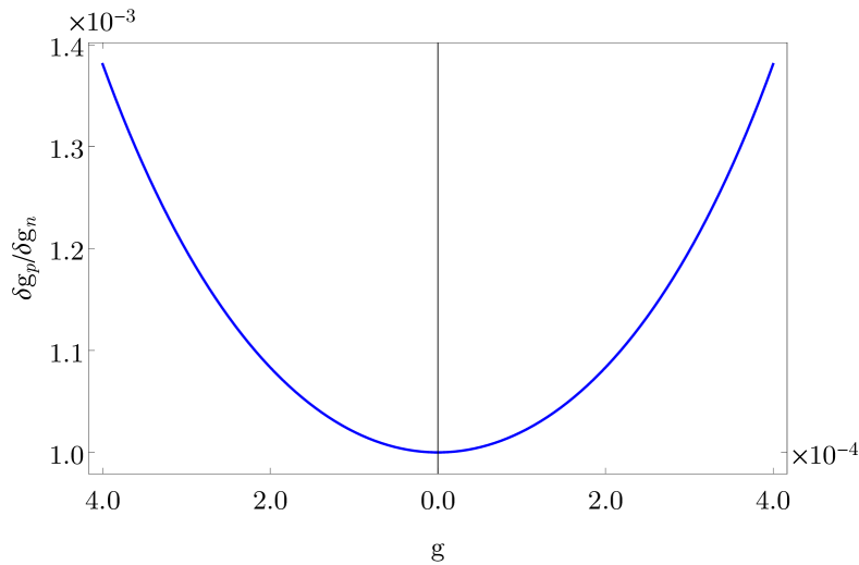
Figure 2: Ratio between the systematic error with and without postselection of the system as a function of the interaction parameter $g$.

Fig. 3 shows the ratio $\frac{\delta g_{p}}{\delta g_{n}}$ with different probe decoherence strength $\epsilon_{D}$ in order to consider the effect of weak value amplification on suppressing systematic errors for different $\epsilon_{D}$. It can be seen from the figure that the suppression rate of systematic error changes very little around $10^{-3}$ for a wide range of $\epsilon_{D}$, which implies that the suppression of systematic error by weak value amplification is very stable with respect to the strength of the probe decoherence.

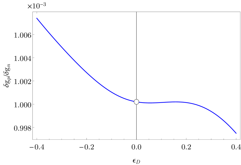
Figure 3: Ratio between the systematic error with and without postselection of the system as a function of the probe decoherence strength $\epsilon_{D}$. $\epsilon_{D}=0$ is removed from the plot, since the systematic errors for both postselected and standard weak measurements are zero at that point, leading to an ill-defined ratio between them.

VI Discussion

In this paper, we mainly considered the systematic error on weak measurement caused by decoherence, and studied the advantage of weak value amplification in suppressing the systematic error of the measurements. We find that a large weak value can effectively suppress the systematic error of postselected weak measurements, compared to standard weak measurement. This is distinct from the loss of Fisher information in the postselected weak measurement under decoherence of the system Knee et al. (2013).

Aside from postselecting the system to one specific state and discarding the unselected results (which was studied in this paper), an alternative method is to retain all the postselection results and use them to estimate the interaction parameter in the Hamiltonian. It has been proven that this method can retain more Fisher information than the method discarding failed postselection results Tanaka and Yamamoto (2013); Combes et al. (2014); Ferrie and Combes (2014); Knee and Gauger (2014); Zhang et al. (2015). This is easy to understand, because the total Fisher information of the data for the estimation is proportional to the size of the data according to the Cramér-Rao bound (23), although in all experimental cases to date, the amount of extra information gained by retaining the other postselection outcomes is negligible Hosten and Kwiat (2008); Dixon et al. (2009); Starling et al. (2009); Viza et al. (2015).

However, the question of whether retaining all postselection results can improve the systematic error in this scenario is more complex. On the one hand, the systematic error is not proportional to the size of data (see Eq. (23)), and the Fisher information in the first-order solution to the systematic error (22) is the average Fisher information of a single event. Therefore, retaining all postselection results, which mixes the events that have high Fisher information and that have low Fisher information, may lead to a lower average Fisher information than postselecting the system, which selects the high Fisher information events only. Thus the systematic error may increase. On the other hand, retaining all postselection results averages the relative entropy between the ideal and the real probability distributions, and the low postselection probabilities for those high Fisher information events could lower the average relative entropy, which may compensate for the loss in average Fisher information. Therefore, it is not clear whether retaining the failed postselection results can in principle improve the systematic error of weak measurement as it does for the Fisher information.

We leave this problem as an open question for future research.