Generalized Second Law of Thermodynamics with Corrected Entropy in Tachyon Cosmology

Abstract

This work is to study the generalized second law (GSL) of thermodynamics in tachyon cosmology where the boundary of the universe is assumed to be enclosed by a dynamical apparent horizon. The model is constrained with the observational data. The two logarithmic and power law corrected entropy is also discussed and conditions to validate the GSL and corrected entropies are obtained.

I introduction

Observations confirm that about two third of the content of the universe is filled with a component dubbed as dark energy (DE) which causes the cosmic expansion to accelerate jarosik . The cosmological constant is the simplest candidate for dark energy which fit the observational data. However, the measured expansion rate of the universe sets its scale being of order of $10^{-12}$GeV, which severely suffers from fine-tuning when compared with the Planck scale ($10^{18}$GeV) shaw . Alternatively, there are a number of DE models which exploit scalar fields or some other exotic fields like phantom fields with negative energy caldwell ; piao . However, such scalar fields are usually so light (or order of $10^{-33}$eV) which need an extremely fine tuning. It is also claimed in the literature, that the cosmic evolution of some kinds of these fields contradict with the solar system tests nojiri . It is most often the case that such fields interact with matter, i) directly due to a Lagrangian coupling, ii) indirectly through a coupling to the Ricci scalar or as the result of quantum loop corrections Damour ; Carroll ; Carroll2 ; bisvas . Recently, a new case has been proposed in which a tachyon scalar field non-minimally couples to matter Lagrangian and the validity of this model in many scenarios has been investigated Faraj1 ; Faraj2 ; Faraj3 ; Faraj4 ; Faraj5 ; Faraj6 .

On the other hand, inspired by the black hole physics, there is a deep connection between gravity and thermodynamics. An evidence for this connection in general relativity (GR) can be shown in deriving the Einstein equations in Rindler spacetime by using the proportionality of the entropy and the horizon area as well as the first law of thermodynamics. Moreover, the validity of the generalized second law of thermodynamics (GSL) Davies ; Pollock ; Pavon1 ; Mukohyama ; Brustein ; Lineweaver ; Izquierdo ; Mohseni ; Gong1 ; Horvat has been under studies. According to GSL, the entropy of the fluid inside the horizon in addition to the entropy associated with the apparent horizon is a nondecreasing function of time. For instance, it is interesting that one can obtain the Friedmann equations by applying the Clasius relation to the apparent horizon of Friedmann-Robertson-Walker (FRW) universe ca . However, it should be mentioned that the definition of entropy would rather be modified in order to include quantum effects motivated from the loop quantum gravity rov ; ash . The modification can be assumed to be a logarithmic or a power-law correction to entropy which consequently leads to appearance of correction terms in derived physical equations, such as modified Newtonian gravity, modified Friedmann equations shey1 ; shey2 ; Deng , and entropic corrections to Coulomb’s law shey3 .

In this paper, the GSL is studied in a general model, first in the standard entropy relation in Section II, and then in the corrected one in both logarithmic and power-law situations in Section III. Then in Section IV, the universe in the presence of a tachyon scalar field non-minimally coupled to matter Lagrangian in the action is considered. The model is constrained with the observational data for distance modulus. In Section V, the GSL is explored by considering the logarithmic and power law corrections to the entropy and with the best-fit parameters.

II The GSL in a general model

Considering the spatially flat Robertson-Walker (RW) metric, the Friedmann equations are

$$3H^{2} = 8\pi\rho$$ (1)

$$2\dot{H}+3H^{2} = -8\pi P.$$ (2)

However, in many cases dealing with a modified action of GR, one can rewrite these equations as

$$3H^{2} = 8\pi\rho_{eff}$$ (3)

$$2\dot{H}+3H^{2} = -8\pi P_{eff},$$ (4)

where $\rho_{eff}$ and $P_{eff}$ are effective density and pressure parameters respectively, which are related together by an effective equation of state parameter, namely $w_{eff}=P_{eff}/\rho_{eff}$.

In what follows, two assumptions are made: i) an entropy is associated with the horizon in addition to the entropy of the universe inside the horizon; ii) according to the local equilibrium hypothesis, there is no spontaneous exchange of energy between the horizon and the fluid inside.

GSL implies that in an expanding universe, the entropy of the viscous DE, dark matter and radiation inside the horizon together with the entropy associated with the horizon do not decrease with time. In general, there are two approaches to validate the GSL on the horizon: i) by applying the first law of thermodynamics to find the entropy relation on the horizon ca ; bous , i.e.,

$$T_{h}dS_{h}=-dE_{h}=4\pi HR^{3}_{h}T_{\mu\nu}K^{\mu}K^{\nu}dt=4\pi(\rho_{eff}+P_{eff})HR^{3}_{h}dt,$$ (5)

where the index $h$ stands for the horizon and $K^{\mu}=(1,-Hr,0,0)$ is the (approximate) Killing vector (the generator of the horizon), or the future directed ingoing null vector field wan ; ii) in the field equations, by employing the horizon entropy and temperature relation on the horizon Bhattacharya ,

$$S_{h} = \pi R^{2}_{h}$$ (6)

$$T_{h} = \frac{1}{2\pi R_{h}}.$$ (7)

Note that only on the apparent horizon are the two approaches equivalent Bhattacharya . Furthermore, the recent observational data from type Ia Supernovae suggests that in an accelerating universe the enclosing surface would be the apparent horizon rather than the event one  zh . Therefore, the universe is assumed to be enclosed by a dynamical apparent horizon with the radius san

$$R_{h}=H^{-1}.$$ (8)

The equation (6) yields the dynamics of the entropy as re ,

$$\dot{S_{h}}=2\pi R_{h}\dot{R_{h}}.$$ (9)

Using (8) as well as the Friedmann equations (3,4) in (9), leads to

$$\dot{S_{h}}=3\pi(1+w_{eff})R_{h}.$$ (10)

On the other hand, applying the fundamental thermodynamics relation to the fluid inside the horizon go gives

$$TdS_{in}=P_{eff}dV+dE_{in}$$ (11)

where $S_{in}$ is the entropy within the apparent horizon, $P_{eff}$ is the effective pressure, $E_{in}=\rho_{eff}V$ is the internal energy, and $V=\frac{4}{3}\pi R^{3}_{h}$. If there is no energy exchange between outside and inside of the apparent horizon, thermal equilibrium occurs that $T=T_{h}$. Therefore, in the case of thermal equilibrium, the relation (11) gives

$$\dot{S_{in}}=\frac{3}{2}\pi(1+w_{eff})(1+3w_{eff})R_{h},$$ (12)

where we use Friedmann equations together with (7) and (8). Table (1) summarizes dependencies of $\dot{S}_{h}$ and $\dot{S}_{in}$ on the equation of state.

	$w_{eff}<-1$	$w_{eff}=-1$	$-1<w_{eff}<-1/3$	$w_{eff}=-1/3$	$w_{eff}>-1/3$
$\dot{S}_{in}$	+	0	–	0	+
$\dot{S}_{h}$	–	0	+	+	+

Table 1: The behaviour of $\dot{S}_{in}$ and $\dot{S}_{h}$ with respect to $w_{eff}$

From Table I, we observe that in cases where the universe is accelerating or crossing phantom line, the rate of change of the entropy inside the apparent horizon and on the apparent horizon is a decreasing function of time. On the other hand, the rate of change of the total entropy, namely the entropy of the horizon plus the entropy within the horizon is

$$\dot{S_{t}}=\frac{9}{2}\pi(1+w_{eff})^{2}R_{h},$$ (13)

which, regardless of the behavior of the apparent horizon radius, is obviously a nondecreasing function of time. The relations (10), (12) and (13) can be re-parameterized as

$$\frac{dS_{X}}{dz}=-\frac{R_{h}}{1+z}\dot{S}_{X},$$ (14)

where $z$ is the redshift and the index $X$ stands for the indices “$in$”, “$h$” and “$t$” respectively. As it is apparent from (14), in an ever-expanding universe, $dS_{X}/dz\lessgtr 0$ whenever $\dot{S}_{X}\gtrless 0$.

III CORRECTIONS TO ENTROPY

As mentioned in standard general theory of relativity, the horizon entropy is proportional to the area of the horizon, i.e. $S=A/4$ where $A=4\pi R_{h}^{2}$. However, modification of the theory, due to the motivation from loop quantum gravity, leads to a correction to the above relation. For instance, in $f(R)$ gravity, the modified entropy is $f^{\prime}(R)A$ Wald . Quantum corrections to the semi-classical entropy law, on the other hand, have been often introduced by logarithmic and power-law terms. In the following contributions from these kinds of corrections will be discussed.

III.1 Logarithmic corrections

Logarithmic corrections, arises from loop quantum gravity due to the thermal equilibrium and quantum fluctuations Miessner ; Ghosh ; Chatterjee ; Banerjee ; Modak ; Jamil ; Sadjadi and as a result the entropy on the apparent horizon become,

$$S_{h}=\frac{A}{4}+\alpha\ln\frac{A}{4}$$ (15)

where $\alpha$ is a dimensionless constant of order unity whose value is still matter of debate. Following the same procedures resulting the relation (10) and (13), one finds the apparent horizon and total entropy as

$$\dot{S_{h}}=3(1+w_{eff})(\pi R_{h}+\frac{\alpha}{R_{h}})$$ (16)

and

$$\dot{S_{t}}=\frac{9}{2}\pi(1+w_{eff})^{2}R_{h}+3\alpha(1+w_{eff})R^{-1}_{h}.$$ (17)

respectively. According to (17), the GSL is satisfied if

$$\alpha\geq\beta\equiv-\frac{3}{2}\pi(1+w_{eff})R^{2}_{h}.$$ (18)

III.2 Power-law corrections

When dealing with the entanglement of quantum fields in and out the horizon, power-law corrections appear, as for example Radicella ; Sheykhi ; Farooq ; Das

$$S_{h}=\frac{A}{4}\left(1-K_{\alpha}A^{1-\frac{\alpha}{2}}\right),$$ (19)

where

$$K_{\alpha}=\frac{\alpha(4\pi)^{\frac{\alpha}{2}-1}}{(4-\alpha)r_{c}^{2-\alpha}}$$ (20)

and $r_{c}$ is the crossover scale. The second term in (19), as a power-law correction to the entropy, has been raised from the entanglement of the wave-functions of a scalar field between its ground state and an exited state. The higher the excitation state the more significant the correction term. It is worth noting that in (20), the correction term tends to zero as the semi-classical limit (large area) is retrieved and consequently the conventional entropy is recovered. The rates of change of the horizon entropy and total entropy are

$$\dot{S_{h}}=3\pi(1+w_{eff})\left(1-K_{\alpha}(4\pi R^{2}_{h})^{1-(2-\frac{\alpha}{2})\frac{\alpha}{2}}\right)R_{h}$$ (21)

and

$$\dot{S_{t}}=\frac{9}{2}\pi(1+w_{eff})^{2}R_{h}-\frac{3}{2}\pi(1+w_{eff})\alpha\frac{R_{h}^{3-\alpha}}{r_{c}^{2-\alpha}}$$ (22)

respectively. Therefore, the GSL will be valid if

$$\alpha\left(\frac{r_{c}}{R_{h}}\right)^{\alpha}\leq 3(1+w_{eff})\left(\frac{r_{c}}{R_{h}}\right)^{2}.$$ (23)

Following Radicella ; Dvali ; Karami ; Hendi , by replacing $r_{c}$ with $R_{h0}$, the above constraint becomes

$$\alpha\left(\frac{R_{h0}}{R_{h}}\right)^{\alpha}\leq 3(1+w_{eff})\left(\frac{R_{h0}}{R_{h}}\right)^{2}.$$ (24)

In the next section, these two corrected version of entropy will be employed to study GSL in the tachyon cosmology in the presence of a non-minimal coupling term to matter.

IV Tachyon Cosmology

The tachyon cosmology with a non-minimal coupling to matter is given by the action:

$$S=\int{d^{4}x\sqrt{-g}\left(\frac{R}{16\pi}-V(\phi)\sqrt{1+g^{\mu\nu}\partial_{\mu}\phi\partial_{\nu}\phi}+f(\phi){\cal{L}}_{m}\right)}$$ (25)

where $R$ is Ricci scalar and $V(\phi)$ denotes the tachyon potential. Unlike the usual Einstein-Hilbert action, the matter Lagrangian ${\cal{L}}_{m}$ is modified as $f(\phi){\cal{L}}_{m}$, where $f(\phi)$ is an analytic function of $\phi$ and causes a non-minimal coupling between the matter and the scalar field. We assume that the mater field filled the universe is cold dark matter and also a spatially flat FRW metric, which forces the tachyon scalar field to be a function of only cosmic time, the field equations become

$$3H^{2}=8\pi\left(\rho_{m}f(\phi)+\frac{V(\phi)}{\sqrt{1-\dot{\phi}^{2}}}\right),$$ (26)

$$2\dot{H}+3H^{2}=-8\pi\left(-V(\phi)\sqrt{1-\dot{\phi}^{2}}\right)$$ (27)

and

$$\ddot{\phi}+(1-\dot{\phi}^{2})\left(3H\dot{\phi}+\frac{V^{\prime}(\phi)}{V(\phi)}\right)=\frac{f^{\prime}(\phi)}{4V(\phi)}(1-\dot{\phi}^{2})^{\frac{3}{2}}\rho_{m}$$ (28)

where prime denotes differentiation with respect to the tachyon field $\phi$.

By using (26) and (28), One can easily arrive at the generalized conservation equation:

$$\dot{(\rho_{m}f(\phi))}+3H\rho_{m}f(\phi)=-1/4\rho_{m}\dot{f}(\phi).$$ (29)

In comparison with (3) and (4), the effective equation of state parameter is identified

$$w_{eff}=\frac{-V(\phi)\sqrt{1-\dot{\phi}^{2}}}{\rho_{m}f(\phi)+\frac{V(\phi)}{\sqrt{1-\dot{\phi}^{2}}}}.$$ (30)

In the following we constrain the parameters of model by using the observational data. Without losing the generality we first rewrite the equations by introducing the following new variables,

$$X=\frac{8\pi\rho_{m}f}{3H^{2}},\quad Y=\frac{8\pi V}{3H^{2}},\quad Z=\dot{\phi},\quad U=\frac{1}{H}.$$ (31)

We assume that $f(\phi)=f_{0}\exp(\delta_{1}\phi)$ and $V(\phi)=V_{0}\exp(\delta_{2}\phi)$ where $\delta_{1}$ and $\delta_{2}$ are dimensionless constants characterizing the slope of the potential $V(\phi)$ and the coupling field $f(\phi)$. Cosmological model with the potentials in the form of exponential functions leading to interesting physics have been used in a variety of contexts, such as accelerating expansion cosmological models do , cosmological scaling solutions se ; chahar ; a ; b , chameleon cosmological models noh ; c , and models with attractor solutions  panj ; d ; e  shesh ; f ; g . Using (26)-(29), the equations for the new dynamical variables become

$$\frac{dX}{dN}=X\left(-1/4\delta_{1}ZU-3Y\sqrt{1-Z^{2}}\right)$$ (32)

$$\frac{dY}{dN}=Y\left(\delta_{2}ZU+3-3Y\sqrt{1-Z^{2}}\right)$$ (33)

$$\frac{dZ}{dN}=\frac{1/4\delta_{1}XU(1-Z^{2})^{\frac{3}{2}}}{Y}-(1-Z^{2})(3Z+\delta_{2}U)$$ (34)

$$\frac{dU}{dN}=\frac{3}{2}U\left(1-Y\sqrt{1-Z^{2}}\right),$$ (35)

where $N=\ln a$ with $a$ being the scalar factor. The Friedmann equation (26), in terms of the new dynamical variables is

$$X+\frac{Y}{\sqrt{1-Z^{2}}}=1.$$ (36)

Using the Friedmann constraint, equations (32)-(35) reduce to

$$\frac{dX}{dN}=X\left(-1/4\delta_{1}ZU-3(1-X)(1-Z^{2})\right)$$ (37)

$$\frac{dZ}{dN}=\frac{1/4\delta_{1}XU(1-Z^{2})}{1-X}-(1-Z^{2})(3Z+\delta_{2}U)$$ (38)

$$\frac{dU}{dN}=\frac{3}{2}U\left(1-(1-X)(1-Z^{2})\right).$$ (39)

Finally, the effective equation of state parameter, as a function of these new variables, is written as

$$w_{eff}=\frac{-Y(1-Z^{2})}{X\sqrt{1-Z^{2}}+Y}.$$ (40)

To constrain the model parameters with the recent observational data, we use “Union2” sample Aman consisting of 557 usable SNe Ia data. The $\chi^{2}$ method, is the method used to best-fit the model for the parameters $\delta_{1}$ and $\delta_{2}$, and the initial conditions $X(0)$, $Z(0)$ and $U(0)$. In this case, the $\chi^{2}$ function is introduced as

$$\chi_{SNe}^{2}(\delta_{1},\delta_{2},X(0),Z(0),U(0))=\sum_{i=1}^{557}\frac{\left[\mu_{i}^{the}(z_{i}|\delta_{1},\delta_{2},X(0),Z(0),U(0))-\mu_{i}^{obs}\right]^{2}}{\sigma_{i}^{2}},$$ (41)

where $\mu_{i}^{the}$ and $\mu_{i}^{obs}$ are the distance modulus parameters obtained from our model and the observations, respectively, and $\sigma$ is the estimated error of $\mu_{i}^{obs}$. It should be mentioned that the difference between the absolute and the apparent luminosity of a distance object is given by

$$\mu(z)=5\log_{10}D_{L}(z)-\mu_{0}$$ (42)

where $\mu_{0}=5\log_{10}h-42.38$ and $h=(H_{0}/100)$km/s/Mpc. The Luminosity distance quantity, $D_{L}(z)$ in (42) is derived as

$$D_{L}(z)=(1+z)H_{0}\int_{0}^{z}\frac{dz^{\prime}}{H(z^{\prime})}.$$ (43)

Table 2, summarizes the results derived by minimizing (41).

Model parameters	X(0)	Z(0)	U(0)	$\delta_{1}$	$\delta_{2}$
Best-fitting results	0.14	0.38	1.43	-0.9	-0.5

Table 2: Best-fit values

V GSL

In this section, by using the best fitted model parameters, the GSL is investigated. Fig. 1 is an illustration of cosmological parameters such as effective EoS parameter in relation to the rate of change of entropy. The graphs are for out model in hand when there is no correction to the entropy. The left panel in Fig. 1, is the graph of $w_{eff}$ versus the redshift $z$. The plot shows that $w_{eff}>-1$ in the;past and future; the universe is currently in quintessence era and it never crosses the phantom barrier. To probe GSL, using (9), (12) and (13), we plot $dS_{h}/dz$, $dS_{in}/dz$ and $dS_{t}/dz$ versus the redshift (the middle panel), and also versus $w_{eff}$ (the right panel) of Fig. 1. The middle graph in Fig. 1 shows the rate of change of entropy within the apparent horizon, on the apparent horizon and total.

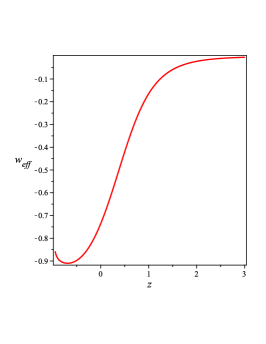
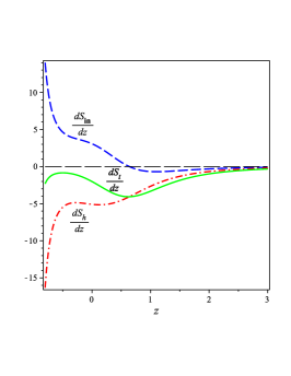
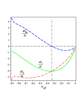
Figure 1: Left: the dynamics of $w_{eff}$ vs. the redshift. Middle: the dynamics of $\frac{dS_{h}}{dz}$, $\frac{dS_{in}}{dz}$ and $\frac{dS_{t}}{dz}$ vs. the redshift. Right: The dynamics of $\frac{dS_{h}}{dz}$, $\frac{dS_{in}}{dz}$ and $\frac{dS_{t}}{dz}$ vs. $w_{eff}$.

In the case of logarithmic corrections, we plot $\beta$, the right hand side of (18), in the left panel of Fig. 2. The constant parameter $\beta$ approaches zero from below. To satisfy GSL, this forces the constant parameter $\alpha$ to be nonnegative as it is apparent from  (18). The right panel of Fig. 2 is an evidence for this claim.

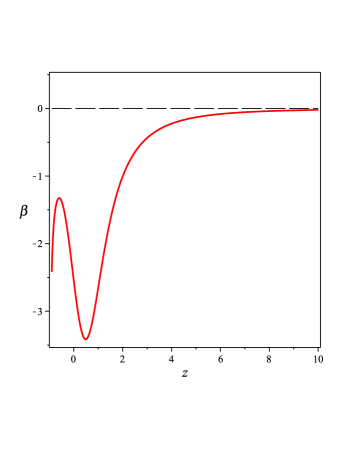
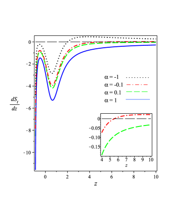
Figure 2: Left: the dynamics of $\beta$ vs. the redshift., and right: the dynamics of $\frac{dS_{t}}{dz}$ vs. the redshift, in logarithmic corrected case for different values of $\alpha$.

Finally, in the case of power-law entropy corrections, we plot $\frac{dS_{t}}{dz}$ against redshift for different values of parameter $\alpha$ in (22). The graphs in Fig. 3 confirm that the GSL is satisfied for $\alpha\leq 0$ . But as $\alpha$ becomes positive, the GSL is violated in the past or future.

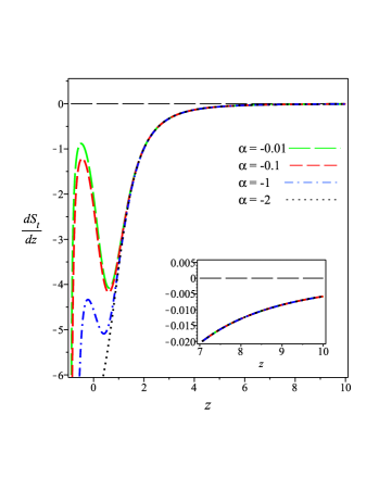
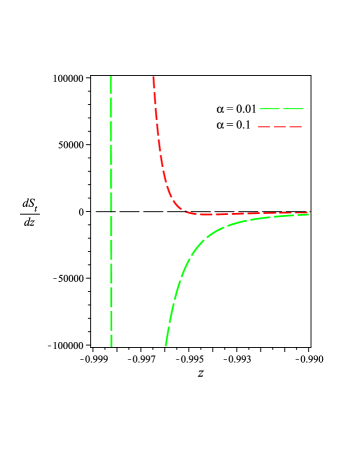
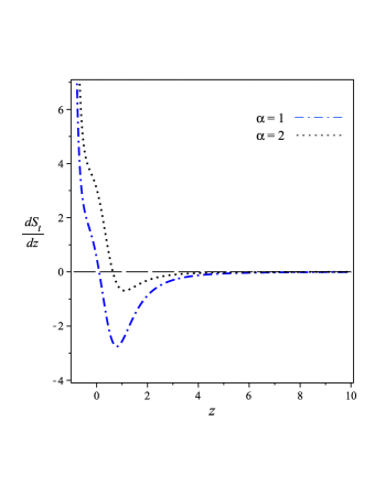
Figure 3: The dynamics of $\frac{dS_{t}}{dz}$ vs. the redshift in power-law corrected case different values of $\alpha\leq 0.1$.

VI Summary and remarks

This paper is intended to study GSL and its corrected version in tachyon cosmological model in the presence of a non-minimal coupling to the matter field. The model is best fitted with the observational data in order to validate the findings. The entropy for the apparent horizon, the fluid inside the universe and the total entropy is obtained. To include quantum effects motivated from loop quantum gravity, two kinds of corrections to the entropy; logarithmic and power law corrections are investigated. In the logarithmic correction, the GSL is satisfied for $\alpha\geq 0$ and in power law for $\alpha\leq 0$. Note that since the best fitted model with observational data reveals no phantom crossing in the past and future the rate of change of entropy of apparent horizon, $dS_{h}/dz$, does not change the behavior and is always positive in accelerating and decelerating eras. On the other hand, the universe begins to accelerate at about $z\simeq-0.6$, and thus the entropy within the horison, $dS_{in}/dz$, changes from negative ( decelerating era) to positive (accelerating era). However,under any circumstances the total entropy variation, $dS_{t}/dz$, is always negative in both cases.

VII Acknowledgment

We would like to thank the university research council of the University of Guilan for financial support.

References

- (1) N. Jarosik et al., ApJS 192, 14 (2011).
- (2) D.J. Shaw and J.D. Barrow, Phys. Rev. D 83, 043518 (2011).
- (3) R. R. Caldwell, Phys. Lett. B. 545, 23 (2002).
- (4) Y. Piao and E. Zhou, Phys. Rev. D. 68, 083515 (2003).
- (5) S. Nojiri and S. D. Odintsov, Mod. Phys. Lett. A. 19, 1273 (2004).
- (6) T. Damour, G. W. Gibbons and C. Gundlach, Phys. Rev. Lett, 64, 123 (1990).
- (7) S. M. Carroll, Phys. Rev. Lett. 81, 3067 (1998).
- (8) S. M. Carroll, W. H. Press and E. L. Turner, Ann. Rev. Astron. Astrophys, 30, 499 (1992).
- (9) T. Biswas, R. Brandenberger, A. Mazumdar and T. Multamaki. Phys. Rev. D. 74, 063501 (2006).
- (10) H. Farajollahi, A. Ravanpak and G. F. Fadakar, Phys. Lett. B. 711, 3-4, 15, 225-231 (2012).
- (11) H. Farajollahi, A. Ravanpak and G. Farrpoor Fadakar, Mod. Phys. Lett. A. 26, 15, 1125-1135 (2011).
- (12) H. Farajollahi, A. Ravanpak and G. F. Fadakar, Astrophys. Space. Sci. 336, 2, 461-467 (2011).
- (13) H. Farajollahi and A. Salehi, Phys. Rev. D. 83, 124042 (2011).
- (14) H. Farajollahi, A. Salehi and A. Shahabi, JCAP. 10, 014 (2011).
- (15) H. Farajollahi, A. Salehi, F. Tayebi and A. Ravanpak, JCAP. 05, 017 (2011).
- (16) P. C. W. Davies, Classical Quantum Gravity 4, L255 (1987).
- (17) M. D. Pollock and T. P. Singh, Classical Quantum Gravity 6, 901 (1989).
- (18) D. Pavon, Classical Quantum Gravity 7, 487 (1990).
- (19) S. Mukohyama, Phys. Rev. D. 56, 2192 (1997).
- (20) R. Brustein, Phys. Rev. Lett. 84, 2072 (2000).
- (21) T. M. Davis, P. C. W. Davies and C. H. Lineweaver, Classical Quantum Gravity 20, 2753 (2003).
- (22) G. Izquierdo and D. Pavon, Phys. Lett. B. 639, 420 (2006).
- (23) H. Mohseni Sadjadi, Phys. Lett. B. 645, 108 (2007).
- (24) Y. Gong, B. Wang and A. Wang , Phys. Rev. D. 75, 123516 (2007).
- (25) R. Horvat, Phys. Lett. B. 648, 374 (2007).
- (26) R. G. Cai and S. P. Kim, JHEP. 02, 050 (2005).
- (27) C. Rovelli, Phys. Rev. Lett. 77, 3288 (1996).
- (28) A. Ashtekar, J. Baez, A. Corichi and K. Krasnov, Phys. Rev. Lett. 80, 904 (1998).
- (29) A. Sheykhi and S. H. Hendi, Phys. Rev. D. 84, 044023 (2011).
- (30) A. Sheykhi, Phys. Rev. D. 81, 104011 (2010).
- (31) B. Liu, Y. C. Dai, X. R. Hu and J. B. Deng, Mod. Phys. Lett. A. 26, 489 (2011).
- (32) A. Sheykhi and S. H. Hendi, Int. J. Theor. Phys. 51, 1125-1136 (2012).
- (33) R. S. Bousso Phys. Rev. D. 71, 064024 (2005).
- (34) Y. Gong, B. Wang and A. Wang, JCAP. 0701, 024 (2007).
- (35) S. Bhattacharya and U. Debnath, gr-qc/1006.2609v1.
- (36) J. Zhou, B. Wang, Y. Gong and E. Abdalla, Phys. Lett. B. 652, 86 (2007).
- (37) R. G. Cai and S. P. Kim, JHEP. 0502, 050 (2005).
- (38) P. C. W. Davies, Classical Quantum Gravity 4, L255 (1987); ibid. 5, 1349 (1988).
- (39) B. Wang, Y. G. Gong and E. Abdalla, Phys. Rev. D. 74, 083520 (2006).
- (40) R. M. Wald, Phys. Rev. D. 48, 3427 (1993).
- (41) K. A. Miessner, Class. Quantum. Grav. 21, 5245 (2004).
- (42) A. Ghosh and P. Mitra, Phys. Rev. D. 71, 027502 (2004).
- (43) A. Chatterjee and P. Majumder, Phys. Rev. Lett. 92, 141301 (2004).
- (44) R. Banerjee and S. K. Modak, JHEP. 0905, 063 (2009).
- (45) S. K. Modak, Phys. Lett. B. 671, 167 (2009).
- (46) M. Jamil and M. U. Farooq, JCAP. 03, 001 (2010).
- (47) H. M. Sadjadi and M. Jamil, Europhys. Lett. 92, 69001 (2010).
- (48) N. Radicella and D. Pavon, Phys. Lett. B. 691, 121 (2010).
- (49) A. Sheykhi and M. Jamil, Gen. Rel. Grav. 43, 2661 (2011).
- (50) M. U. Farooq and M. Jamil, Canadian J. Phys. 89, 1251 (2011).
- (51) S. Das, S. Shankaranarayanan and S. Sur, Phys. Rev. D. 77, 064013 (2008).
- (52) G. Dvali and M. S. Turner, arXiv:astro-ph/0301510 (2003).
- (53) K. Karami, A. Abdolmaleki, N. Sahraei and S. Ghaffari, JHEP. 1108, 150 (2011).
- (54) A. Sheykhi and S. H. Hendi, Phys. Rev. D. 84, 044023 (2011).
- (55) J. J. Halliwell, Phys. Lett. B. 185, 341 (1987).
- (56) B. Ratra and P. J. E. Peebles, Phys. Rev. D. 37, 3406 (1988).
- (57) J. Yokoyama and K. I. Maeda, Phys. Lett. B. 207, 31 (1988).
- (58) A. A. Coley, J. Ibanez and R. J. van den Hoogen, J. Math. Phys. 38, 5256 (1997).
- (59) V. D. Ivashchuk, V. N. Melnikov, and A. B. Selivanov, JHEP. 0309, 059 (2003).
- (60) P. Brax, C van de Bruck, A. C. Davis, J. Khoury and A. Weltman, Phys. Rev. D. 70, 123518 (2004).
- (61) J. Khoury and A. Weltman, Phys. Rev. D. 69, 044026 (2004).
- (62) W. Fang, Y. Li, K. Zhang and H. Q. Lu, Class. Quant. Grav. 26, 155005 (2009).
- (63) K. Maeda and Y. Fujii, Phys. Rev. D. 79, 084026 (2009).
- (64) I. P. C. Heard and D. Wands, Class. Quant. Grav. 19, 5435-5448 (2002).
- (65) T. Barreiro, E. J. Copeland and N. J. Nunes, Phys. Rev. D. 61, 127301 (2000).
- (66) A. A. Sen and S. Sethi, Phys. Lett. B. 532, 159 (2002).
- (67) U. Franca and R. Rosenfeld, JHEP. 0210, 015 (2002).
- (68) R. Amanullah, et al., Astrophys. J. 716, 712 738 (2010).