Direct Ejecta Velocity Measurements of Tycho’s Supernova Remnant

Abstract

We present the first direct ejecta velocity measurements of Tycho’s supernova remnant (SNR). Chandra’s high angular resolution images reveal a patchy structure of radial velocities in the ejecta that can be separated into distinct redshifted, blueshifted, and low velocity ejecta clumps or blobs. The typical velocities of the redshifted and blueshifted blobs are $\lesssim 7,800$ km s^-1 and $\lesssim 5,000$ km s^-1, respectively. The highest velocity blobs are located near the center, while the low velocity ones appear near the edge as expected for a generally spherical expansion. Systematic uncertainty on the velocity measurements from gain calibration was assessed by carrying out joint fits of individual blobs with both the ACIS-I and ACIS-S detectors. We determine the three-dimensional kinematics of the Si- and Fe-rich clumps in the southeastern quadrant and show that these knots form a distinct, compact, and kinematically-connected structure, possibly even a chain of knots strung along the remnant’s edge. By examining the viewing geometries we conclude that the knots in the southeastern region are unlikely to be responsible for the high velocity Ca II absorption features seen in the light echo spectrum of SN 1572, the originating event for Tycho’s SNR.

1. Introduction

The X-ray emission from remnants of Type Ia supernovae (SNe) holds important clues about the nature of these explosions, which are used as standardizeable candles to determine the expansion history of the Universe (Riess et al., 1998; Perlmutter et al., 1999). Additionally there is increasing evidence that the high-speed shock waves driven by these explosions accelerate cosmic rays to PeV energies (see Slane et al., 2014, for the specific case of Tycho’s supernova remnant). To investigate these two important scientific questions, measurements of key dynamical quantities, such as ejecta bulk velocity flows, turbulence, and ion temperatures, are critical, yet such measurements are extremely challenging to make with current instrumentation.

Tycho’s supernova remnant (SNR), recorded by Tycho Brahe in 1572 and studied by him for more than a year, is known to be the result of a type Ia supernova (SNIa) based, circumstantially, on the light curve from Tycho’s observations (Baade, 1945; Ruiz-Lapuente et al., 2004) and, definitively, on the light-echo spectrum obtained with modern instrumentation (Krause et al., 2008). As the prototypical Galactic example of a SNIa explosion, Tycho’s SNR has been well studied for insights into the SNIa explosion mechanism. Badenes et al. (2006) made a detailed comparison between the ejecta X-ray emission properties of Tycho’s SNR and several SNIa explosion models. They concluded that the X-ray morphology and integrated spectrum was well reproduced by a one-dimensional delayed detonation model with compositionally stratified ejecta, expanding into a uniform ambient medium density with density $\rho\sim 2\times 10^{-24}$ g cm^-3. Some collisionless electron heating at the reverse shock ($\beta\equiv T_{e}/T_{\rm ion}\sim 0.03$) was necessary to explain the XMM-Newton and Chandra observations. In this model, the mean velocity of the shocked ejecta was estimated to be $\sim$2000 km s^-1.

The expansion velocities of the forward shock and shocked ejecta have also been studied through proper motion measurements. Hughes (2000) made the first accurate X-ray expansion rate measurement by comparing the brightness profiles from two observations by the ROSAT high resolution imager taken in 1990 and 1995. This indicated expansion rates of 0.22^′′–0.44^′′ yr^-1 at the outer rim of Tycho, where the range represents the variation in expansion rate from the peak of the ejecta emission to the remnant’s edge. Katsuda et al. (2010) used Chandra observations to measure the expansion rates of both the forward-shock and the ejecta. They found the proper motion of the reverse-shocked ejecta to be 0.21–0.31^′′ yr^-1, consistent with the earlier ROSAT work. Converting these rates into shock velocities requires knowledge of the remnant’s distance which remains uncertain with a spread of published values mostly between 2 kpc and 4 kpc (see Hayato et al., 2010, for a review of distance determinations to Tycho’s SNR). For reference, an angular expansion rate of 0.26^′′ yr^-1 corresponds to a velocity of $\sim$3700 km s^-1 for a distance of 3 kpc.

Spectral measurements have also revealed evidence for significant ejecta expansion velocities. Using data from the Suzaku satellite, Furuzawa et al. (2009) and Hayato et al. (2010) found broadened X-ray line spectra from the remnant’s interior, which both studies interpreted as being due to the Doppler shifting of lines from the approaching and receding hemispheres of the SNR. They required expansion velocities of the Si, S and Ar ejecta to be 4700$\pm$100 km s^-1, somewhat larger than the inferred velocity of the Fe ejecta (4000$\pm$300 km s^-1). The ejecta velocities measured by these two different methods (proper motion and line broadening) are broadly consistent and higher than the predicted velocity in Badenes et al. (2006). However, direct measurements of ejecta velocities in Tycho’s SNR have not been done yet.

In this paper, we aim to directly measure the velocities of the shocked ejecta with Chandra. From high angular resolution X-ray imaging over the years (e.g., with Einstein, ROSAT and Chandra), clumpy ejecta structures have been clearly noted in Tycho’s SNR (e.g., Seward et al., 1983; Vancura et al., 1995; Hwang et al., 2002). It is plausible to suspect that such clumps could have different velocities along the line of sight as a result of, for example, being located on either the approaching or receding side of the remnant. If so it should be possible to separate these with a sufficiently good combination of X-ray imaging and spectroscopy.

This paper is organized as follows. The next section discusses the observations used and the data reduction procedures applied to the data. In §3 we present our imaging and spectroscopic analysis of the data and results on ejecta velocities in Tycho’s SNR. Section 4 places our results in the broader context and the final section concludes. An Appendix presents an additional validation test of our ejecta velocity measurements with Chandra. Throughout this article uncertainties are quoted at the 90% confidence level, unless explicitly stated otherwise.

2. Observation and Data Reduction

2.1. Chandra ACIS-I and ACIS-S Data Sets

The Chandra Advanced CCD Imaging Spectrometer Imaging-array (ACIS-I, Garmire et al., 1992; Bautz et al., 1998) observed Tycho’s SNR in April 2009 (PI: Hughes) for a effective exposure of 734.1 ksec. The observation was carried out using nine ObsIds as summarized in Table 1. We reprocessed all the level-1 event data, applying standard data reduction procedures using tasks from version 4.7 of the Chandra Interactive Analysis of Observations (CIAO) package with calibration data from the version 4.6.1 CALDB. For spectral extraction, we used specextract and made weighted response files using this script. The default aspect solution for each ObdID was used; previous work has shown that the relative registration for the ObsIDs of this Tycho data set is good (Eriksen et al., 2011). Unless otherwise stated, background was taken from the exterior detector area beyond a radius of 4.75 arcmin centered on the remnant. Fits were done using XSPEC 12.8.2 and AtomDB 2.0.2.

Table 1Log of Chandra Observations Used in this Study

		Date	Exposure	Roll Angle
Detector	ObsID	(YYYY/MM/DD)	time (ks)	(deg)
ACIS-S	115	2000/09/20	48.9	171.0
ACIS-I	10093	2009/04/13	118.4	29.2
”	10094	2009/04/18	90.0	29.2
”	10095	2009/04/23	173.4	29.2
”	10096	2009/04/27	105.7	29.2
”	10097	2009/04/11	107.4	26.3
”	10902	2009/04/15	39.5	29.2
”	10903	2009/04/17	23.9	29.2
”	10904	2009/04/13	34.7	29.2
”	10906	2009/05/03	41.1	37.2
ACIS-I	sum	$\ldots$	734.1	$\ldots$

Table 2Log of Suzaku Observations Used in this Study

		Date	Exposure (ks)
Name	ObsID	(YYYY/MM/DD)	[XIS0+3]	SCI
Tycho’s SNR	500024010	2006/06/27	202.2	off
”	503085020	2008/08/11	205.7	on
E0102$-$72	100044030	2006/02/02	42.6	off
”	103001030	2008/08/12	22.6	on

In addition to the frontside-illuminated CCD chips on ACIS-I, Chandra carries a spectroscopic array (ACIS-S) with a backside-illuminated chip that can be used for imaging. An observation of Tycho’s SNR using ACIS-S was carried out early in the mission for an effective exposure time of 48.9 ks (see Table 1). The effective area and spectral resolution of the ACIS-I and ACIS-S detectors are quite different; additionally the two detectors allow us to sample two independent sets of readout electronics for the spectra of individual features in the remnant. Therefore we utilized both detectors as a powerful cross-check of our spectral results and to establish the level of systematic error in derived velocities. Data reduction and analysis techniques for the ACIS-S data were the same as for ACIS-I.

2.2. Suzaku XIS

For an additional comparison with the Chandra data, we also analyzed data from the X-ray Imaging Spectrometers (XIS, Koyama et al., 2007) onboard Suzaku. The Suzaku XIS observed Tycho’s SNR twice as summarized in Table 2. The primary data reduction was performed following the standard procedures recommended by the instrument team as implemented in the aepipeline task (using HEASOFT version 6.16). Ancillary response files (arf) and redistribution matrix files (rmf) were generated using xissimarfgen and xisrmfgen, respectively. For calculating the XIS effective area, we assumed the Chandra image in the 1.6–2 keV band as the input sky map. For spectral analysis, we used only the XIS data of the front-illuminated CCDs (XIS0 and 3). Background data were taken from the nearby source-free sky area and subtracted from the source spectrum.

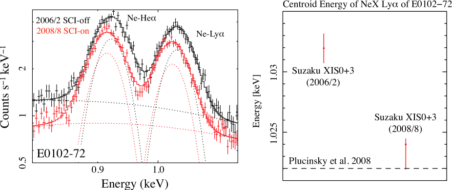
Figure 1.— Left: Suzaku spectra of E0102$-$72 in the vicinity of the Ne X Ly$\alpha$ line from observations taken in 2006 and 2008. Right: Comparison of the centroid energy of the Ne X Ly$\alpha$ line between 2006 and 2008. The dashed horizontal line shows the expected Ne X Ly$\alpha$ line energy of E0102$-$72 from high spectral resolution observations (Plucinsky et al., 2016).

From October 2006, the XIS observed using the Spaced-row Charge Injection mode (SCI: Uchiyama et al., 2009). The two observations of Tycho’s SNR were therefore observed in each of these different modes. We found a discrepancy in the fitted line centroid energy between these two modes. Figure 1 (left panel) shows the XIS spectra of the calibration source SNR E0102$-$72 in these epochs over the energy band that contains the Ne IX He$\alpha$ and Ne X Ly$\alpha$ lines. Fits were done using individual Gaussian models for the two line features plus a powerlaw continuum. The Ne X Ly$\alpha$ line centroid in the 2006 observation is inconsistent by $\sim$10 eV (Figure 1 - right panel) with the value determined by Plucinsky et al. (2016), who use high spectral resolution grating instruments to characterize E0102$-$72’s 0.3–2.5 keV band emission and establish this source as an effective calibration standard. The centroid energy from our analysis of the 2008 data is, however, consistent with Plucinsky et al. (2016).

3. Data Analysis and Results

3.1. Radial Profile

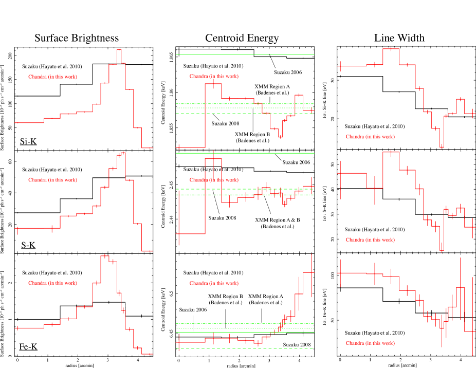
Figure 2.— Radial profile of surface brightness, centroid energy and line width. Top, middle and bottom show the Si-He$\alpha$, S-He$\alpha$ and Fe-K$\alpha$ lines, respectively. We divided the whole SNR into 12 “Sky” regions. Black curves show the results from Suzaku (Hayato et al., 2010), while the red curves show the Chandra results from this work. The regions from the innermost to the outermost are referred to as Sky1–Sky12. The regions were all centered on the geometric center of the remnant: 00^h25^m19^s, 64^∘08^′10^′′ (J2000). The outer radii of the Sky1–Sky12 regions were 0.87^′, 1.41^′, 1.95^′, 2.49^′, 2.76^′, 3.03^′, 3.3^′, 3.44^′, 3.58^′, 3.85^′, 4.12^′ and 4.66^′, respectively. The Sky1 to Sky2 regions were complete circles/annuli. For the remaining regions (Sky3 to Sky12), we excluded the southeast portion of the remnant corresponding to position angles between 60^∘ and 150^∘. Uncertainties are shown at the 90 % confidence level. Solid (dashed) green lines show the best-fit values of centroid energy from the entire SNR from 2006 (2008) Suzaku observation. Dash-dotted and dotted green lines show the XMM-Newton results from regions A and B, respectively from Badenes et al. (2006).

In this section, we check the consistency of the radial profiles of line properties from our Chandra analysis with past results and, because of Chandra’s sharper point-spread-function (PSF), we also investigate finer radial dependencies. Figure 2 shows the radial profiles of the surface brightness, centroid energies and line widths of the K$\alpha$ line blends of Si, S and Fe from Chandra (red curves). The black curves show the Suzaku profiles (Hayato et al., 2010). Four radial bins were used in that work. In our analysis, we divided essentially the same area into 12 radial bins (referred to later as Sky1 through Sky12). Chandra spectral fits followed the same procedure as used in the Suzaku analysis: a set a broadened Gaussian lines and a powerlaw continuum fit over the energy range 1.7–3.4 keV for the Si+S band and 5.0–7.0 for the Fe band, which also includes the Cr K line. Specifically the lines we included as Gaussians were Si-He$\alpha$, Si-Ly$\alpha$, Si-He$\beta$, Si-He$\gamma$, S-He$\alpha$, S-Ly$\alpha$, S-He$\beta$ and Ar-He$\alpha$(+S-He$\beta$) in the Si+S band and Cr-K$\alpha$ and Fe-K$\alpha$ in the Fe band. We treated the He-like complexes as single broadened Gaussians with their centroid energies and normalizations as free parameters. The line widths of the prominent He$\alpha$ blends of Si, S, Ar were fitted freely. For the other blends (e.g., He$\beta$, He$\gamma$ and Ly$\alpha$), we fixed the line width to the He$\alpha$ value. The intensity, centroid, and width of the Fe-K$\alpha$ line were free parameters; the width of the Cr-K$\alpha$ line was fixed to that of the Fe line. We note that the energy centroid of the Fe K$\alpha$ line in Tycho is $\sim$6.4 keV and corrresponds to a mean ionization state of Fe XVII (Yamaguchi et al., 2014); over the entire remnant it can be described well by a single broadened Gaussian line.

The radial bins in the Chandra profiles are all fully independent, unlike the Suzaku profiles where the broader PSF of the Suzaku X-ray telescope (with a half-power diameter of $\sim$2^′) causes significant amounts of flux to mix from one bin to the others. Consequently, we obtain much sharper surface brightness profiles than Suzaku. We found that the Si-He$\alpha$ and the S-He$\alpha$ lines peak in intensity at a radius of $\sim$3.3^′–3.5^′, consistent with XMM-Newton (Decourchelle et al., 2001). We note that the S-He$\alpha$ line appears to peak at a slightly higher radius than the Si-He$\alpha$ line. For Fe-K$\alpha$, we found an intensity peak at a radius of $\sim$3.0^′, which is also consistent with past results (e.g., Warren et al., 2005; Yamaguchi et al., 2014).

The energy centroid profiles are shown in the middle columns of Figure 2. Again the Chandra profiles are shown in red and the published Suzaku ones are in black. The green lines show other values integrated over the remnant from the literature (XMM: Badenes et al., 2006) or our own analysis of the 2006 and 2008 Suzaku data. For the Si and S line centroid energies, the new Chandra profiles are inconsistent with the Suzaku data taken in 2006, which are $\sim$10 eV too high. This is also the data set with inconsistent line centroids for the calibration target E0102$-$72, so we are justified in ignoring it for this consistency check. Since the Chandra profiles are consistent with all the other data sets, we are confident that the energy scale of the Chandra observation is accurate.

In principle, for a perfectly uniform emitting shell, the energy centroid profiles should be flat. In fact, however, the Chandra profiles show significant radial structure. One notable feature is the statistically significant jump in centroid energy from the innermost bin to the second one. For the Si-He$\alpha$ line, this jump is $\sim$9 eV, which corresponds to a difference in line-of-sight velocity of $\sim$1450 km s^-1. This value is about 30% of the expansion speed of the Si-rich shell and it can be explained if we assume that there is an factor of approximately two difference in the intrinsic intensity of the approaching and receding hemispheres in this radial bin. We propose that the patchy nature of the remnant’s emission is the source of the structures seen in the Si and S line centroid profiles. We consider this in further detail in § 3.5 below. We also consider the increasing Fe line centroid energy beyond the peak emission below (§ 4.3).

For the line width profile, we found a gradual decrease from the center toward the edge. This feature was also seen (albeit at lower resolution) by Suzaku (Furuzawa et al., 2009; Hayato et al., 2010); these authors interpreted the variation of the line width radial profile as the signature of an expanding shell of ejecta. An important new feature of the Chandra profiles is the clear minimum in the line width at a radius of $\sim$3.4^′ (the Sky8 region). This is also where the line intensity peaks. We identify this as the region where the ejecta are moving most closely to the plane of the sky and therefore show little to no Doppler shift.

3.2. Expansion Velocity

Table 3Best-fit Parameters of the Double Gaussian Model from the Central Regions Using Chandra

	Width	$E_{\rm red}$	$E_{\rm blue}$	2$\delta E$	$v_{\perp}$	$v_{\rm exp}$ (km s-1)	$v_{\rm exp}$ (km s-1)
Lines	(eV)	(keV)	(keV)	(eV)	(km s-1)	(this work)	(Hayato et al. 2010)
Si-He$\alpha$	12.6	1.821$\pm$0.003	1.880${}^{+0.002}_{-0.003}$	59$\pm$4	4780$\pm$320	5010$\pm$340	4730${}^{+30}_{-20}$
S-He$\alpha$	15	2.393${}^{+0.006}_{-0.009}$	2.478${}^{+0.004}_{-0.006}$	87${}^{+7}_{-11}$	5240${}^{+430}_{-680}$	5490${}^{+450}_{-710}$	4660$\pm$50
Fe-K$\alpha$	41	6.36$\pm$0.02	6.53$\pm$0.02	170$\pm$30	4000$\pm$700	4200$\pm$800	4000$\pm$300
Using only high surface brightness pixels
Si-He$\alpha$	12.6	1.822$\pm$0.003	1.884${}^{+0.002}_{-0.003}$	62$\pm$4	5020$\pm$320	5260$\pm$340	—
S-He$\alpha$	15	2.389$\pm$0.007	2.478${}^{+0.004}_{-0.005}$	89${}^{+8}_{-9}$	5490${}^{+490}_{-550}$	5750${}^{+510}_{-580}$	—
Using only low surface brightness pixels
Si-He$\alpha$	12.6	1.821${}^{+0.004}_{-0.005}$	1.880${}^{+0.003}_{-0.004}$	59${}^{+4}_{-5}$	4780${}^{+320}_{-410}$	5010${}^{+340}_{-430}$	—
S-He$\alpha$	15	2.395${}^{+0.008}_{-0.009}$	2.479${}^{+0.007}_{-0.008}$	84${}^{+11}_{-12}$	5170${}^{+680}_{-740}$	5410${}^{+710}_{-770}$	—

Here we estimate the shell expansion velocity from the Si, S, and Fe K lines using the Chandra data from the center of Tycho’s SNR, extracting the spectrum from within a radius of 1.41^′ (Sky1 plus Sky2 regions) to match the previous work with Suzaku. We modeled the line broadening as in previous work (Hayato et al., 2010) with two Gaussian lines corresponding to the Doppler-shifted components from the receding and approaching hemispheres of the expanding shell of ejecta. The faint lines (specifically Ly$\alpha$, He$\beta$ and He$\gamma$) were included in several ways: as single narrow or broadened lines, or as narrow lines linked in velocity to the corresponding red- or blueshifted He$\alpha$ line. We also allowed the width of each of the double He$\alpha$ Gaussian lines to vary within the allowed range from the Sky8 region fits (${}^{+0.5}_{-0.6}$ eV for Si-He$\alpha$ and $\pm$2 eV for S-He$\alpha$). In all cases the derived energy differences between the red- and blueshifted components for both Si and S were in agreement. The final uncertainty on the energy difference includes the statistical uncertainty plus the range from the different spectral models. Results of the Chandra fits for the three species are given in Table 3 (for now we only consider the top three entries that correspond to the integrated spectrum from the central region). For the Si+S band the best fit yields $\chi^{2}=146.75$ for 92 degrees of freedom and for the Fe band $\chi^{2}=137.32$ for 127 degrees of freedom. Figure 3 shows that the double Gaussian model is a good fit to the spectra data.

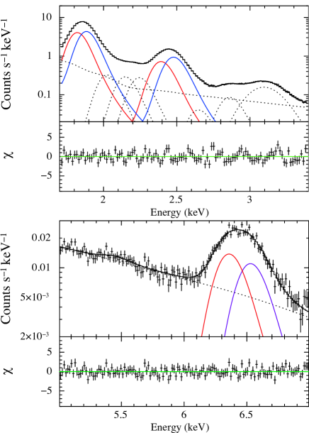
Figure 3.— Double Gaussian model fit to the Chandra spectrum from the center of Tycho’s SNR (Sky1+Sky2 regions) in the Si+S band (top panel) and the Fe-K$\alpha$ band (bottom panel). The weak bump at $\sim$5.6 keV in the bottom panel is Cr K$\alpha$ line emission. The continuum emission is fitted with a power-law model.

For the spectral fits, line widths were fixed at the values determined from the minima in each radial profile. The radial velocity ($v_{\perp}$) was calculated from the average energy of the red- and blue-shifted components and $\delta E$. To convert $v_{\perp}$ to the shell expansion speed we needed to correct for the projection factor over the central 1.41^′ of the remnant. For Si-He$\alpha$ and S-He$\alpha$, we assumed a spherically symmetric shell extending over 190^′′–220^′′ and for Fe-K$\alpha$, we assumed the shell covered the radial range 180^′′–200^′′. We calculated the projection factor using the method in section A.1 of Hayato et al. (2010). We determined projection factors of 0.955 for Si-He$\alpha$ and S-He$\alpha$ and 0.948 for Fe-K$\alpha$. For Suzaku, an additional correction was necessary to account for the flux spreading due to the broad Suzaku PSF. This can be ignored for the Chandra analysis.

The shell expansion velocities from Chandra are in the range of $\sim$4200–5500 km s^-1; all are consistent with the Suzaku results. The large uncertainty on the Fe shell expansion from Chandra alone does not allow us to exclude that it is moving at the same speed as the other species. However, by combining all of the Si and S measurements (both Chandra and Suzaku, i.e., using a weighted combination of the values in the last two columns of Table 3) we arrive at an expansion velocity for the Si+S shell of $4724^{+27}_{-19}$ km s^-1 that is significantly greater ($>$4$\sigma$) than the (similarly combined) Fe-shell expansion velocity of $4025\pm 280$ km s^-1.

The results quoted above correspond to an emission-measure-weighted mean velocity difference for the approaching and receding hemispheres. Although this is a practical approach from an observational perspective, it may not produce an unbiased result. If, for example, there is a correlation between expansion speed and emission-measure (say, because higher intensity spots, such as compact blobs of ejecta, tend to expand more quickly) then we will get a biased velocity difference. However, thanks to Chandra’s high angular resolution we can assess this effect. We divided all pixels within the central 1.41^′ region by surface brightness into either high or low values (splitting at the mean level of $\sim$$6\times 10^{-4}$ ph s^-1 cm^-2 arcmin^-2) and extracted a separate spectrum for each pixel set. Results for the Si and S lines are given in the bottom entries of Table 3 and in all cases (Si and S, high and low surface brightness), the velocity differences are statistically in agreement with the result from the integrated spectrum. This suggests that in general there is not a strong correlation between expansion speed and the brightness of features through the center of Tycho’s SNR.

3.3. Mean Photon Energy Map of Si-He$\alpha$

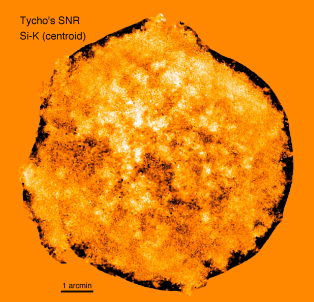
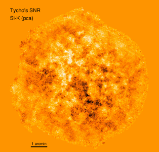
Figure 4.— Left: Mean photon energy map in the Si-He$\alpha$ band (1.6–2.1 keV) from the deep Chandra ACIS-I observation of Tycho’s SNR. Voroni Tessellation was used to combine pixels to produce varying-sized regions with similar signal-to-noise ratio in each region. We chose a S/N of 20 for this image (i.e., approximately 400 detected Si line photons). The color scale varies linearly from energy centroid values of 1.816 keV (dark) to 1.879 (light). The dark ring around the edge is where nonthermal dominates over thermal emission. Right: Map of the Si-He$\alpha$ band data projected onto the Principal Component that separates red- and blue-shifted emission (see text). The color scale here has been adjusted to approximately match that in the left panel.

Small clumpy structures in the ejecta in Tycho’s SNR have been noted since the Einstein Observatory High Resolution Imager observations in the late 1970s (e.g., Seward et al., 1983). We consider here the possibility that these structures or blobs might have different expansion speeds which would be manifest as differences in line centroid energy due to the Doppler effect. For this we used the Si-He$\alpha$ line because of its large statistical signal.

We divided the 1.6–2.1 keV band into 34 energy bins (each 15 eV in width) and made fluxed images at each energy using the merge_obs script in CIAO. We computed the mean photon energy in each bin using

$$E_{\rm mean}=\frac{\sum_{i}E_{i}I_{i}}{\sum_{i}I_{i}},$$

where $E_{i}$ and $I_{i}$ are the photon energy and the intensity at each energy bin ($i=1,2,...,34$). To equalize the signal-to-noise across the map, we used Voroni Tessellation (e.g., Cappellari & Copin, 2003; Diehl & Statler, 2006) to merge pixels together to reach a uniform signal-to-noise ratio of 20 in each bin. Hereafter we refer to these as VT bins.

Figure 4 (left panel) shows the mean photon energy map for the Si-He$\alpha$ line in Tycho’s SNR. The image is dominated by patchy structures that, in many cases but not all, can be associated with specific features in the intensity map. There is some striping in the image that correlates with the readout direction of the chips (toward the NE and SW), but this effect is clearly subdominant to the patchy structure of the remnant. The dark region around the rim of the remnant is where nonthermal continuum emission dominates; we do not remove the continuum in our map-making procedure so these regions are not correct in this map. The maximum range of mean photon energy values is $\gtrsim$60 eV, which corresponds to a range of ejecta velocities of $\gtrsim$9,700 km s^-1. This is quite close to twice the Si-He$\alpha$ expansion velocity determined above (see Table 3).

We have also done a Principal Components Analysis (PCA) of the Si-He$\alpha$ band images following closely the previous application of this method to Tycho’s SNR (Warren et al., 2005). In our application here, we generated a large number of Si-He$\alpha$ line spectra (one from each VT bin) and compressed each from 34 spectral bins into 18 by summing together bins in the fainter wings of the line profile. These spectra were input to the PCA algorithm (Murtagh & Heck, 1987) to identify new axes in the 18-dimensional space of the data set that maximized its variance.

As discussed by Warren et al. (2005), there is no guarantee, in general, that the Principal Components (PCs) identified by PCA have a unique astrophysical interpretation. However, in this case of a specific emission line, we found that the first three PCs have spectral templates with a clear and unequivocal interpretation: (1) line equivalent width, (2) line energy centroid, and (3) line energy width. There are as many PCs as spectral bins (18 here) and in the case of a totally random dataset, each PC would account for $\sim$6% of the variance of the full data set. Here we found that the first three PCs each account for 17%, 15% and 6% of the variance with the remaining components each accounting for less than 5%. We conclude therefore that the first two PCs are significant, the third is marginal, and that the remaining PCs are all insignificant.

A map of the Chandra Si-He$\alpha$ spectral data projected onto the second PC is shown in Figure 4 (right panel). This map closely matches the mean centroid map shown in the left panel validating our interpretation of it as being due to line centroid variations. The agreement between the two maps is poor near the outer rim, where continuum emission causes the centroid calculation to produce spurious results.

Together these maps indicate that there is enough variation in the Si-He$\alpha$ line centroids to motivate identifying individual red- and blue-shifted blobs and measuring their velocities through spectral analysis. We turn to this in the next section.

3.4. Spectral Analysis of Specific Blobs

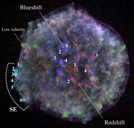
Figure 5.— Three-color image of the Si-He$\alpha$ line from the Chandra ACIS-I observation of Tycho’s SNR. The red, green and blue images come from the 1.7666–1.7812 keV, 1.8396–1.8542 keV, and 1.9564–1.971 keV bands. Magneta, blue, and green circles identify the redshifted, blueshifted and low velocity blobs, respectively, used for the spectral analysis. Likewise the cyan circles show the knots in the southeastern quadrant that we studied.

Figure 5 shows a color image of Tycho’s SNR constructed from three narrow energy slices of the Si-He$\alpha$ line as noted in the figure caption. In this figure, we see two kinds of Si-He$\alpha$ blobs in the central region: blobs with higher (bluish color) or lower (reddish color) photon energy. We defined appropriately sized, circular regions (r = 0.1^′) for these blobs and extracted their spectra (shown in Figure 6). There is a clear separation of the centroid energies between the red- and the blue-shifted blobs. Rough eyeball estimates for the Si-He$\alpha$ and the S-He$\alpha$ lines suggest centroid energy differences of $\sim$60 eV and $\sim$70 eV, respectively, or Doppler velocity differences of $\sim$9,000 km s^-1.

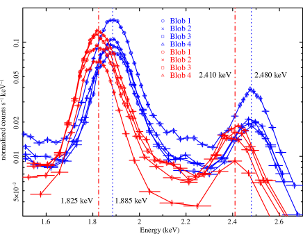
Figure 6.— Typical spectra of the red- and blue-shifted blobs. The symbol types and numeric labels correspond to the regions from which the spectra were extracted shown on Figure 5. Vertical bars show the 1 $\sigma$ uncertainty on intensity; horizontal bars just indicate the size of the energy bin.

In addition to the Doppler effect, line centroids are also sensitive to the shock-heating history of the line-emitting material. In particular the ionization age (which is the product of the electron density and the time since the material was shock heated, $n_{e}t$) can affect the prominence of the H-like Ly$\alpha$ line and, for lower values, can also affect the energy centroid of the He-like complex. Increasing the ionization age tends to increase the mean charge state which tends to increase the centroid of the K line. However, over rather wide ranges of ionization ages, the charge state is dominated by the He-like species (as in the case of Tycho’s SNR) and the dependence of line centroid on ionization age is weak. Furthermore, increases in charge state from He-like to H-like produce noticeable distortions in the shape of the Si K line (i.e., making it double peaked) even at CCD spectral resolution. We see no significant evidence for such line shape distortions in the PCA results (i.e., the significant PCs correspond to the first three moments of the line: intensity, centroid, and width, while there are no significant PCs corresponding to higher moments, such as skewness or bimodality), so large ionization age variations are not expected.

Nevertheless, to separate Doppler shifts from any possible ionization state changes, we carried out detailed spectral analyses using nonequilibium ionization (NEI) models. We extracted the spectra from 27 regions in total including the red- and blue-shifted blobs mentioned above, as well as several low velocity blobs near the edge of Tycho’s SNR. These were fitted with the vnei model (for the NEI thermal component) and the srcut model (for the nonthermal continuum component) in XSPEC. Also, we allowed for the model spectra to be broadened using the gsmooth model since thermal broadening and/or multiple Doppler components might be present. For the srcut model, we assumed a constant radio spectral index of $\alpha=-0.65$ (Kothes et al., 2006) based on the integrated flux densities at 408 and 1420 MHz and allowed the cutoff frequency and radio intensity to be free parameters. Absorption due to the intervening column density of interstellar material is negligible in this band ($>$1.6 keV) so we ignored it for these fits.

Figure 7 shows a scatter plot of the best-fit line-of-sight velocity versus the ionization age for each blob. The maximum separation of blob velocity reaches $\sim$9000 km s^-1 even taking into account the variability of the ionization age. From the thermal model, the ionization ages are in the range of $\sim 10^{10}$–$10^{11}$ cm^-3 s, and electron temperatures are $\sim$0.9–2.7 keV (mean $kT\sim$1.3 keV). We also analyzed a number of blobs close to the edge of the remnant. These blobs have smaller velocities than the blobs from the interior, but a similar range of ionization timescales. The pattern of line-of-sight velocities shown in Figure 7 is consistent with the effect of projection on the line-of-sight velocities and agrees qualitatively with the results in Figure 2.

The detector gain for ACIS is monitored and updated by regular observation of the external ⁵⁵Fe source onboard Chandra. However, since there is no simultaneous, independent gain reference for the ACIS-I detector during any specific observation, we are potentially subject to uncalibrated gain variations. In order to assess this effect we extracted matched spectra of 8 blobs from the ACIS-S detector and fit them using the same model as above. In this analysis, we initially conducted a joint fit between the ACIS-I and the ACIS-S data for each blob. Then we linked all parameters except for the gsmooth and redshift parameters and fitted for independent values of the broadening and velocity.

The ACIS-S spectral fitting results are shown in Figure 7 using the same symbol types as for the ACIS-I results, except now with dashed error bars. Table 4 gives the sky locations of the jointly fitted blobs, their locations on the detector (i.e., CCD chip and readout node), and the best-fit velocity for the two data sets. We obtained similar velocities in the two ACIS data sets. There is a discrepancy of $\sim$500–2,000 km s^-1 in the sense that the ACIS-S detector tends to yield more redshifted spectra than ACIS-I. However, even when averaging all of the velocity measurements, we still see a velocity difference of $>$8,000 km s^-1 between the red- and blue-shifted blobs. Thus we conclude that our spectral separation of the red- and the blue-shifted components correspond to intrinsic velocity differences in Tycho’s SNR. Velocity measurements, however, carry a systematic uncertainty of $\sim$500–2,000 km s^-1. Improvements of the ACIS gain calibration may help to reduce this systematic error.

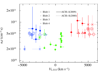
Figure 7.— Scatter plot between the line-of-sight velocity and the ionization age ($n_{e}t$) for each blob. Velocities are based on the vnei model “redshift” parameter. The open symbols, identification numbers, and red or blue colors correspond to the 8 regions in Figure 6. Solid and dashed error bars show results from the ACIS-I and ACIS-S detectors, respectively. The filled circles show the results of the other 19 regions in Figure 6 and the colors correspond to redshifted (red), blueshifted (blue) or low velocity (green) blobs.

Table 4Summary of Joint ACIS-I and ACIS-S Spectral Analysis of Red- and Blue-shifted Blobs

			ACIS-I		ACIS-S	Sky Background		Blob Local Background
	id	(R.A., Decl.)	chip	node	node	$V_{\rm I}$ [km s-1]	$V_{\rm S}$ [km s-1]	$V_{\rm I}$ [km s-1]	$V_{\rm S}$ [km s-1]
Blueshifted blobs						(Mean: $-3220\pm$970)		(Mean: $-4310\pm$880)
	Blob1	(00h25m24s.952, 64∘09′33′′.76)	2	0	1	$-3616^{+4}_{-88}$	$-2390^{+700}_{-140}$	$-4880^{+140}_{-30}$	$-3440^{+700}_{-140}$
	Blob2	(00h25m24s.843, 64∘09′21′′.72)	2	0	1	$-4730^{+30}_{-190}$	$-2400^{+10}_{-1100}$	$-5030^{+170}_{-40}$	$-3350^{+30}_{-160}$
	Blob3	(00h25m28s.633, 64∘08′37′′.08)	2	0	1, 2	$-4000^{+190}_{-180}$	$-3370^{+60}_{-190}$	$-5040^{+140}_{-50}$	$-4910^{+90}_{-900}$
	Blob4	(00h25m25s.275, 64∘08′25′′.04)	2, 3	0, 3	1	$-3700^{+80}_{-40}$	$-1550^{+420}_{-500}$	$-5030^{+50}_{-70}$	$-2790^{+500}_{-900}$
	Blob5	(00h25m27s.538, 64∘07′57′′.05)	0, 1, 2	0, 3	—	$-3540^{+200}_{-660}$	—	—	—
	Blob6	(00h25m28s.710, 64∘07′39′′.33)	0, 1	0, 3	—	$-3010^{+580}_{-420}$	—	—	—
	Blob7	(00h25m06s.514, 64∘08′25′′.35)	3	3	—	$-2370^{+26}_{-40}$	—	—	—
	Blob8	(00h25m04s.715, 64∘07′52′′.27)	3	3	—	$-2984^{+4}_{-1}$	—	—	—
Redshifted blobs						(Mean: $+4980\pm$740)		(Mean: $+7230\pm$840)
	Blob1	(00h25m16s.180, 64∘07′58′′.82)	3	3	1	$+5200^{+480}_{-150}$	$+5840^{+470}_{-100}$	$+7780^{+420}_{-220}$	$+7580^{+710}_{-310}$
	Blob2	(00h25m14s.237, 64∘06′50′′.80)	1	0	1	$+5020^{+20}_{-140}$	$+5650^{+690}_{-300}$	$+7580^{+710}_{-210}$	$+7420^{+1870}_{-680}$
	Blob3	(00h25m04s.588, 64∘08′49′′.07)	3	2, 3	0	$+4950\pm 90$	$+5550^{+200}_{-150}$	$+7580^{+680}_{-180}$	$+7610^{+1480}_{-170}$
	Blob4	(00h25m07s.629, 64∘07′50′′.99)	3	3	0, 1	$+3500^{+260}_{-320}$	$+4150^{+680}_{-90}$	$+5040^{+140}_{-110}$	$+7210\pm 330$
	Blob5	(00h25m14s.709, 64∘08′43′′.20)	0, 1	0, 3	—	$+2420^{+50}_{-190}$	—	—	—
	Blob6	(00h25m26s.368, 64∘07′35′′.43)	1	0	—	$+3360^{+450}_{-130}$	—	—	—
	Blob7	(00h25m14s.237, 64∘06′50′′.80)	1, 3	0, 3	—	$+4510^{+140}_{-430}$	—	—	—
	Blob8	(00h25m09s.489, 64∘06′44′′.50)	3	3	—	$+4110^{+430}_{-30}$	—	—	—
Low velocity blobs
	Blob1	(00h25m41s.454, 64∘11′11′′.91)	2	0, 1	—	$+850^{+30}_{-40}$	—	—	—
	Blob2	(00h25m43s.965, 64∘09′39′′.19)	0, 2	0, 3	—	$-1700^{+390}_{-10}$	—	—	—
	Blob3	(00h25m52s.184, 64∘09′43′′.82)	0, 2	0, 3	—	$-40^{+120}_{-50}$	—	—	—
	Blob4	(00h25m35s.171, 64∘05′17′′.71)	1	1	—	$+810^{+481}_{-3}$	—	—	—
	Blob5	(00h25m23s.641, 64∘04′38′′.78)	1	1	—	$+811^{+117}_{-1}$	—	—	—
	Blob6	(00h25m14s.187, 64∘04′44′′.08)	1	0, 1	—	$+930^{+350}_{-30}$	—	—	—
	Blob7	(00h24m59s.954, 64∘05′14′′.10)	1	0, 1	—	$+780^{+20}_{-340}$	—	—	—
	Blob8	(00h24m52s.735, 64∘05′57′′.71)	1, 3	0, 3	—	$-780^{+270}_{-60}$	—	—	—
	Blob9	(00h24m45s.049, 64∘07′10′′.81)	3	2, 3	—	$-1710^{+50}_{-20}$	—	—	—
	Blob10	(00h25m51s.594, 64∘09′15′′.48)	3	2	—	$+910^{+10}_{-130}$	—	—	—
	Blob11	(00h24m43s.913, 64∘09′33′′.67)	3	2	—	$+60^{+30}_{-390}$	—	—	—

Finally we consider the possibility of contamination of a blob’s spectrum from material in the extraction region at a different velocity (from, for example, the other side of the shell). Such contamination would tend to reduce a blob’s observed velocity compared to its actual velocity. To assess this effect, we extracted local background spectra from regions near each blob (the fits presented above used spectra of blank-sky regions from beyond the remnant’s edge) and carried out the spectral fits with the new background spectra. In Table 4, we summarize the fit results under the columns labeled “Blob Local Background.” Not surprisingly we found best-fit velocities higher by $\sim$1,000-2,000 km s^-1 than with the traditional blank-sky background. Additionally best-fit line widths were smaller. In the case of the blank-sky background, line widths were in the range of $\sim$20–40 eV, while with the local blob background, line widths were typically a factor of two lower and generally consistent with the minimum line widths obtained from the Sky8 region (see Figure 8 for the comparison). These results suggest that there is some contamination from different velocity components in the blob spectra and that the actual velocities of the blobs could be as high as in the last two columns (“Blob Local Background”) of Table 4. However, the highly structured nature of the X-ray emission on arcsecond scales makes a precise determination of the amount of contaminating material in any individual blob’s spectrum difficult to do in practice. However, as an ensemble, it is plausible to conclude that fits using local blob background spectra provide reasonable upperbounds on the velocities of the red- and blue-shifted blobs of $\lesssim 7,800$ km s^-1 and $\lesssim 5,000$ km s^-1, respectively.

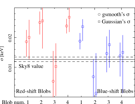
Figure 8.— Best-fit Si-He$\alpha$ line widths for 8 individual blobs using local regions near each blob for background. Circle (box) symbols show the results of fits using the gsmooth (Gaussian lines) model. Solid and dashed lines show the best-fit value and 90% confidence level uncertainty from the Sky8 region.

3.5. Large Scale Distribution of Apparent Ejecta Velocity

Here we focus on the large scale velocity structure of Tycho’s SNR. Inspection of the mean photon energy map (Figure 4 shows an obvious asymmetry in the distribution of red- and blue-shifted blobs between the northern and southern sides. This asymmetry is also clearly visible in the ACIS-S data (image not shown).

When the remnant is divided into northern and southern parts (using the two green semicircular regions shown in Figure 9, left), we find different mean energies: $\sim$1.860 kev from the north and $\sim$1.851 keV from the south (Figure 9 right). The mean energy of the Si-He$\alpha$ line at the edge of the remnant (in the Sky8 region where the line width is minimum), determined using the same method, is $\sim$1.856 keV, which is approximately halfway between the energies of the two halves just determined. Taking this energy as the “rest frame” of Tycho’s SNR we find that the bulk of the northern and southern halves appear to be moving along the line-of-sight at $\sim$$\pm$700 km s^-1 with respect to this frame.

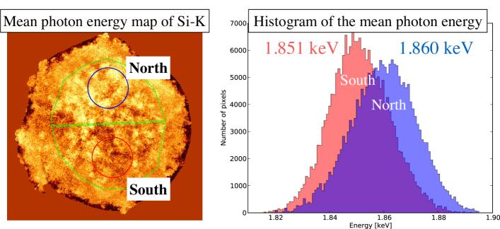
Figure 9.— Left: definition of the northern and southern side regions with the mean photon energy map. Two green polygon regions are used for making the histogram. Two circles are used for the spectral analysis. Right: the histogram of the number of pixels in the two green semicircular regions as shown in the left figure.

Table 5Line Centroid Energies in the Northern and Southern Regions of Tycho’s SNR with Chandra & Suzaku

	ACIS-I	ACIS-S	Suzaku
Si-He$\alpha$
North (keV)	1.8634$\pm$0.0003	1.8613$\pm$0.0005	1.8571${}^{+0.0003}_{-0.0002}$
South (keV)	1.8493$\pm$0.0003	1.8490$\pm$0.0007	1.8545$\pm$0.0003
$\delta E$ (eV)	14.1$\pm$0.4	12.3$\pm$0.9	2.7${}^{+0.4}_{-0.3}$
$\delta V$ (km s-1)	2280$\pm$60	1990$\pm$150	440${}^{+60}_{-50}$
S–He$\alpha$
North (keV)	2.4494$\pm$0.0007	2.4481${}^{+0.0035}_{-0.0027}$	2.4506${}^{+0.0017}_{-0.0010}$
South (keV)	2.4318${}^{+0.0017}_{-0.0014}$	2.4282${}^{+0.0047}_{-0.0030}$	2.4441${}^{+0.0016}_{-0.0014}$
$\delta E$ (eV)	17.6${}^{+1.8}_{-1.6}$	19.9${}^{+5.9}_{-4.0}$	6.5${}^{+2.3}_{-1.7}$
$\delta V$ (km s-1)	2160${}^{+220}_{-200}$	2450${}^{+730}_{-490}$	800${}^{+280}_{-210}$
Fe-K$\alpha$
North (keV)	6.452${}^{+0.006}_{-0.007}$	6.435${}^{+0.014}_{-0.012}$	6.430$\pm$0.005
South (keV)	6.413$\pm$0.006	6.415$\pm$0.014	6.420${}^{+0.006}_{-0.007}$
$\delta E$ (eV)	39${}^{+8}_{-9}$	19${}^{+20}_{-19}$	10${}^{+8}_{-9}$
$\delta V$ (km s-1)	1820${}^{+370}_{-420}$	890${}^{+930}_{-890}$	690${}^{+550}_{-620}$

To examine this issue in more detail we extracted ACIS-I, ACIS-S, and Suzaku XIS spectra from the two circular regions shown in Figure 9 (the northern region is centered at [R.A., Decl.] = [00^h25^m17^s.519, 64^∘10^′06^′′.53], the southern one is at [R.A., Decl.] = [00^h25^m15^s.581, 64^∘06^′41^′′.07], and both regions are 1 arcmin in radius). Fits were done using the same Gaussian model as in § 3.1. Results are given in Table 5. We found a strong tendency for the northern region to have higher centroid energies than the southern region. Of particular note is the excellent numerical consistency between the ACIS-I and ACIS-S detectors, which demonstrates that this effect is not an observational artifact. For the Si-He$\alpha$ and S-He$\alpha$ line, the difference of centroid energies corresponds to a line-of-sight velocity difference of $\sim$2000 km s^-1. The result for the Suzaku XIS is not as large due to the smoothing induced by Suzaku’s broad PSF.

Before jumping to the conclusion that this velocity difference implies a kinematic asymmetry in the original SN explosion, we first must explore the possibility that the velocity difference is due to the patchy nature of the ejecta shell. Recall that we interpret the fluctuations in the mean line centroid in the radial profiles (Figure 2) in this way. We can estimate the average velocities in the northern and southern regions assuming different relative amounts of emission from the approaching and receding hemispheres using this simple algebraic function

$$\langle v_{N,S}\rangle=\frac{v_{\rm red}I_{{\rm red},N,S}+v_{\rm blue}I_{{\rm blue},N,S}}{I_{{\rm red},N,S}+I_{{\rm blue},N,S}},$$

where the labels “red” and “blue” indicate the red and blueshifted components, the labels “N” and “S” refer to the northern and southern sides, and $I$ is the line intensity from each of the four relevant locations. Then $\langle v_{N,S}\rangle$ are the average speeds in each region. Next we define the relative intensity ratio $\chi_{N,S}\equiv I_{{\rm blue},N,S}/I_{{\rm red},N,S}$ allowing us to define the difference of the average velocities between the northern and southern regions as

$$\langle v_{N}\rangle-\langle v_{S}\rangle=v\left(\frac{1-\chi_{N}}{1+\chi_{N}}-\frac{1-\chi_{S}}{1+\chi_{S}}\right),$$

where we have made the simplest assumption that the north and south regions have the identical expansion speed, $v$, along the line of sight. We choose the northern and southern circular regions to be offset symmetrically from the center so this assumption is reasonable. Because of the offset, the radial speed in each region is less than the shell expansion speed (Table 3), by a projection factor. For a Si shell radius of $\sim$3.4^′ the offset location of the circular regions ($\sim$1.7^′) yields a projection factor to the line-of-sight of $\cos\,30^{\circ}=0.866$, which yields a projected speed of $v\sim 4000$ km s^-1. The observed north-south velocity difference is $\sim$ $-2000$ km s^-1, so the value in the parentheses of the above equation is $-0.5$. This value can be accommodated by a range of front-back intensity ratios for the north and south in the (physically plausible) range $\chi_{N}=1/3$ and $\chi_{S}=0$ to $\chi_{N}=3$ and $\chi_{S}=1$. The most modest intensity ratio differences are $\chi_{N}=5/3$ and $\chi_{S}=3/5$, less than a factor of two for each side.

Thus a biased intensity distribution for a uniformly expanding shell of ejecta can account for the observed north to south velocity difference in Tycho’s SNR. And the biased intensity distribution is not necessarily the result of an asymmetric explosion, since local variations in the ambient medium density can result in significant local intensity differences in the ejecta. A higher ambient medium density is likely why the ejecta emission is so much brighter in the northwest quadrant of Tycho’s SNR (see, e.g., Katsuda et al., 2010). To explain the velocity difference, we suggest that this enhancement extends over the front (blueshifted) part of the shell but not over the back (redshifted) part. This would require that the mean ejecta density be $\lesssim$ $\sqrt{3}$ higher in the front than the back, which is plausible given the estimated ambient density enhancement of a factor of $\sim$2 in the northwest (Katsuda et al., 2010).

3.6. Velocities of Southeastern Knots

The southeastern (SE) quadrant of Tycho’s SNR is morphologically and compositionally different from the rest of the remnant. For example, the bright knots in the SE are located at a radius of $\sim$4.2^′, which is $\sim$20%-30% further out from the center than the peak Si-He$\alpha$ and Fe-K$\alpha$ line intensity over the rest of the remnant. In addition, the SE knots show strong differences in relative Si to Fe abundances (e.g., Vancura et al., 1995; Decourchelle et al., 2001; Warren et al., 2005). Here we study the kinematic properties of compact knots in this region, focusing on the six knots identified in Figure 5 (cyan circles).

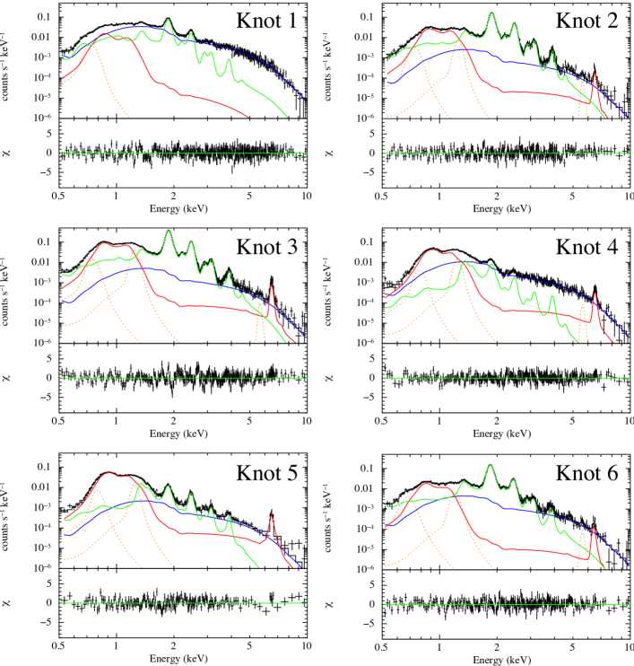
Figure 10.— X-ray spectra and the best-fit models for the southeastern knots in Tycho’s SNR. Labels in each panel (e.g., Knot1, Knot2, and so on) correspond to the region number in Figure 5. Green and red curves show the model for the IME component and the iron component, respectively. Blue curves show the power-law continuum model. Orange dashed curves show the additional Gaussian models. Error bars on the spectra are shown at 1 $\sigma$

Table 6Fit Results for the Southeastern Knots

Parameter	Knot1	Knot2	Knot3	Knot4	Knot5	Knot6
R.A.	00h25m53s.647	00h25m57s.141	00h25m56s.998	00h25m57s.509	00h25m57s.627	00h25m51s.481
Decl.	64∘08′10′′.69	64∘07′47′′.42	64∘07′32′′.52	64∘07′05′′.03	64∘06′45′′.35	64∘05′42′′.36
$\chi^{2}$/d.o.f	433/379	302/254	476/305	248/286	198/163	307/265
$N_{\rm H}$ (1022cm-2)	0.55$\pm$0.05	0.59${}^{+0.03}_{-0.02}$	0.61$\pm 0.01$	0.65${}^{+0.05}_{-0.01}$	0.66${}^{+0.01}_{-0.04}$	0.48${}^{+0.03}_{-0.01}$
Line broadening (eV)	29$\pm$2	23$\pm$1	25$\pm$1	16${}^{+6}_{-9}$	15${}^{+5}_{-6}$	24$\pm$2
Velocity (km s-1)	$-$2330${}^{+270}_{-10}$	$-$2410${}^{+10}_{-100}$	$-$2393${}^{+2}_{-10}$	$-$1880${}^{+180}_{-100}$	$-$1050${}^{+90}_{-160}$	$+$900${}^{+50}_{-110}$
IME component
$kT_{\rm e}$ (keV)	2.6${}^{+2.1}_{-1.0}$	1.3$\pm 0.1$	1.23$\pm$0.04	0.75$\pm$0.03	0.60$\pm$0.01	1.7${}^{+0.3}_{-0.2}$
$n_{\rm e}t$ (1010cm-3 s)	2.0${}^{+0.5}_{-0.3}$	4.8${}^{+0.7}_{-0.2}$	5.1$\pm$0.2	28${}^{+41}_{-5}$	1000	3.1$\pm$0.6
${\rm[Mg/C]/[Mg/C]}_{\odot}$	1.4${}^{+0.6}_{-0.3}$	5.8$\pm$0.9	2.8$\pm$0.1	360$\pm 30$	110$\pm$6	32${}^{+36}_{-2}$
${\rm[Si/C]/[Si/C]}_{\odot}$	9${}^{+4}_{-2}$	120${}^{+40}_{-20}$	61$\pm$10	430${}^{+160}_{-40}$	140${}^{+9}_{-7}$	430${}^{+490}_{-10}$
${\rm[S/C]/[S/C]}_{\odot}$	10${}^{+5}_{-3}$	160${}^{+40}_{-20}$	80$\pm$13	480${}^{+100}_{-110}$	400${\pm 30}$	430${}^{+20}_{-160}$
${\rm[Ar/C]/[Ar/C]}_{\odot}$	7${}^{+5}_{-3}$	180${}^{+80}_{-30}$	79$\pm$5	870${}^{+2900}_{-720}$	780${}^{+190}_{-180}$	320$\pm 50$
${\rm[Ca/C]/[Ca/C]}_{\odot}$	22${}^{+20}_{-14}$	400${}^{+180}_{-70}$	180$\pm$20	4000${}^{+6000}_{-3000}$	2000${}^{+8000}_{-1000}$	900${}^{+700}_{-200}$
norm $\int n_{e}n_{\rm C}dV/4\pi d^{2}/[{\rm C}/{\rm H}]_{\odot}$ ($10^{9}$ cm-5)	6${}^{+4}_{-2}$	1.9${}^{+1.1}_{-0.7}$	8.8${}^{+0.1}_{-0.6}$	0.057${}^{+0.61}_{-0.001}$	0.39${}^{+0.57}_{-0.01}$	0.36${}^{+0.23}_{-0.01}$
Fe component
$kT_{\rm e}$ (keV)	1.2${}^{+2.0}_{-0.5}$	8.6${}^{+0.5}_{-1.4}$	9.3$\pm$0.1	9.2${}^{+0.4}_{-0.2}$	9.1$\pm 0.1$	10${}^{+7}_{-1}$
$n_{\rm e}t$ (1010cm-3 s)	2${}^{+3}_{-1}$	1.31$\pm$0.05	1.09$\pm$0.03	1.58$\pm$0.03	1.52${}^{+0.04}_{-0.02}$	0.97$\pm$0.08
${\rm[Fe/C]/[Fe/C]}_{\odot}$	1.1${}^{+0.9}_{-0.4}$	5.8${}^{+1.0}_{-0.9}$	4.8${}^{+0.9}_{-0.1}$	360${}^{+9600}_{-10}$	70${}^{+110}_{-2}$	18.4${}^{+4.8}_{-0.7}$
norm $\int n_{e}n_{\rm C}dV/4\pi d^{2}/[{\rm C}/{\rm H}]_{\odot}$ ($10^{9}$ cm-5)	6	1.9	8.8	0.057	0.39	0.36
power-law component
$\Gamma$	2.71${}^{+0.06}_{-0.05}$	2.4$\pm 0.3$	2.45${}^{+0.07}_{-0.06}$	2.83$\pm$0.03	2.59${}^{+0.09}_{-0.06}$	2.3${}^{+0.2}_{-0.1}$
norm ($\times 10^{-5}$ ph keV-1 cm-2 s-1 at 1 keV)	32$\pm 2$	2.3${}^{+1.1}_{-0.7}$	4.6$\pm$0.5	11.80${}^{+0.14}_{-0.03}$	2.2$\pm 0.2$	3.6$\pm$0.6
Additional lines
Fe L + O K Center (keV)	0.73${}^{+0.02}_{-0.03}$	0.74${}^{+0.02}_{-0.01}$	0.75$\pm$0.01	0.78$\pm$0.01	0.80$\pm$0.01	0.68${}^{+0.02}_{-0.01}$
Fe L + O K norm ($\times 10^{-6}$ ph cm-2 s-1)	5$\pm 2$	3.5${}^{+0.9}_{-1.1}$	13.9$\pm$1.6	3.3${}^{+0.7}_{-0.8}$	5.5${}^{+0.7}_{-1.2}$	6.0${}^{+1.4}_{-1.6}$
Fe L Center (keV)	—	1.25$\pm$0.01	1.247$\pm$0.004	1.242$\pm$0.006	1.247$\pm$0.006	1.21${}^{+0.03}_{-0.01}$
Fe L norm ($\times 10^{-6}$ ph cm-2 s-1)	—	1.9${}^{+0.5}_{-0.3}$	11.2$\pm$0.7	4.1${}^{+0.7}_{-1.3}$	4.0$\pm 0.4$	2.5${}^{+1.0}_{-1.1}$
Cr K Center (keV)	—	5.6${}^{+0.6}_{-0.1}$	5.65${}^{+0.14}_{-0.21}$	5.61$\pm$0.11	—	5.61${}^{+0.62}_{-0.10}$
Cr K norm ($\times 10^{-8}$ ph cm-2 s-1)	—	7$\pm$6	9$\pm$8	8$\pm$8	—	10$\pm 9$

We extracted the spectra from these circular regions (with radius 0.1^′) and fit them over the 0.5–10 keV energy band with a two component NEI model, power-law continuum, and additional Gaussian lines. The two NEI models account for iron emission separately from the intermediate-mass elements (IMEs), Si, S, Ar, and Ca. We link the redshift parameters for the two NEI components. We assume no hydrogen, helium, or nitrogen in the shocked SN Ia ejecta and quote abundances with respect to carbon (the lowest atomic number species that we include in our spectral analysis). Oxygen and neon are kept fixed at their solar value with respect to carbon; the abundances of the other species are allowed to be free. Several Gaussian lines at $\sim$0.7 keV, $\sim$1.2 keV and $\sim$5.6 keV were added to account for missing lines, such as Fe-L ($n=3s,3d\rightarrow 2p$ for Fe XVIII as shown in Gu et al., 2007) and/or O-K (K-shell transition lines higher than K$\delta$ as shown in Yamaguchi et al., 2008), Fe-L ($n=6,7,8\rightarrow 2$ for Fe XVII, $n=6,7\rightarrow 2$ for Fe XVIII, and $n=6\rightarrow 2$ for Fe XIX as shown in Brickhouse et al., 2000; Audard et al., 2001), and Cr-K$\alpha$, respectively, in the atomic databases. Line broadening of the plasma models is included using the gsmooth model, and the broadening of the additional Gaussian lines is linked to the same value. Absorption is included assuming solar abundances (Anders & Grevesse, 1989).

The spectral data and best-fit models are shown in Figure 10 and numerical values of the fit parameters are given in Table 6. The quoted abundances are relative to carbon relative to the solar value and in nearly all cases, as expected for SN Ia ejecta, are much greater than unity. This model provided good results (with $\chi^{2}$/d.o.f $<$ 1.6), and has highlighted some differences among the knots. Knot2, Knot3, and Knot6 are more Si-rich, while Knot4 and Knot5 are more Fe-rich; both points are consistent with previous results. Knot1 is dominated by nonthermal emission compared to both the Si and Fe thermal components. The velocities of the Si-rich and Fe-rich knots are $\sim-$2400 km s^-1 and $\sim-$1900 to $-$1100 km s^-1, respectively. This is unexpected for a spherical expansion, where the edge of the shell should have no velocity along the line of sight. These results suggest that the SE knots are in fact inclined to the plane of the sky and are therefore moving faster than their proper motion would imply. We return to this point below. Of course the reader should keep in mind the systematic uncertainty of $\sim$500–2000 km s^-1 in the velocities of individual blobs as demonstrated in section 3.4.

4. Discussion

Thanks to the high angular resolution of Chandra, we have obtained (1) a more detailed view of the radial profiles of line centroid and width, (2) consistency of our expansion velocity measurements with previous results and (3) clear identification of red- and blue-shifted components on multiple angular scales in Tycho’s SNR. These basic results hold the hope of advancing our understanding of the type Ia SNe mechanism. In this section, we begin this effort as we consider the implications of our results for the distance to Tycho’s SNR, the origin and nature of the southeastern (SE) knots, and the shock heating processes in the ejecta.

4.1. Distance to Tycho’s SNR

The expansion rate of Tycho’s SNR has been studied using proper motion measurements from X-ray imaging. Katsuda et al. (2010) investigated the expansion rates of both the forward-shock and the reverse-shocked ejecta using Chandra ACIS high-resolution images of Tycho’s SNR obtained in multiple epochs. For the reverse-shocked ejecta, they presented proper motion measurements for five azimuthal sectors around the rim for two sets of epoch pairs (see Table 3 in Katsuda et al., 2010). We use the 2003–2007 comparison (since it uses the same instrument ACIS-I for both epochs) and average their five azimuthal results to arrive at a mean proper motion of $\mu=(0.267\pm 0.056)^{\prime\prime}$ yr^-1. The uncertainty here is taken to be the standard deviation of the five azimuthal values (multiplied by 1.6 to approximate the 90% confidence level), rather than the uncertainty on the mean. Combining this with our expansion velocity of 5010$\pm$340 km s^-1, we estimate an allowed range on the distance to Tycho’s SNR of $D=(4.0\pm 0.3~{}^{+1.0}_{-0.7})(V/5010{\rm~{}km~{}s}^{-1})(\mu/0.267^{\prime\prime}{\rm~{}yr}^{-1})$ kpc, where the first and second terms show the uncertainties from expansion velocity and proper motion. This is consistent with the result from Suzaku (Hayato et al., 2010): 4 $\pm$ 1 kpc as well as the result based on the SN peak luminosity, as established by the observed optical light-echo spectrum, and the maximum apparent brightness from the historical records: 3.8${}^{+1.5}_{-1.1}$ kpc (Krause et al., 2008).

Although the Chandra expansion speed measurement seems redundant in that it reproduces the apparently more precise value from Suzaku, it is important to note that the Suzaku result is subject to a correction factor due to that telescope’s large PSF that is completely eliminated in the case of Chandra. Additionally, the high angular resolution of Chandra has allowed us to assess whether there is an intensity-dependent bias in the measured velocity difference, which might arise if, for example, brighter blobs tended to move at higher or lower speeds than fainter ones. We find that this is not a concern. The velocity difference between high and low surface brightness regions in the central region of Tycho’s SNR is small (less than 10%) and not statistically significant.

Estimating the remnant’s distance from the individual blob analyses will be more uncertain due to the several systematic effects on the velocity measurements (see §3.4) and because of difficulty in identifying an appropriate matched sample of knots with good proper motion measurements.

4.2. High Velocity Knots in the Southeastern Quadrant

The SE quadrant is one of the most mysterious features in Tycho’s SNR, and it is not yet understood how such a prominent structure could be made. An aspherical explosion is one of the possibilities. Theorists have found a number of ways to produce asymmetric SN Ia explosions, including, pre-explosion convection (Kuhlen et al., 2006), off-center ignition of the burning front (Maeda et al., 2010; Röpke, Woosley, & Hillebrandt, 2007), and gravitationally confined detonations (Plewa, Calder, & Lamb, 2004; Jordan et al., 2008). On the observational front, Maeda et al. (2010) have argued for large scale explosion asymmetries to explain the diversity in the spectral evolution of SN Ia. In addition to Tycho’s SNR, the elemental composition in SN 1006 inferred from Suzaku observations also appears to be asymmetric Uchida et al. (2013).

The light-echo spectrum of Tycho’s SNR Krause et al. (2008), spectrum shows a high velocity feature (HVF) identified as the Ca II triplet at a velocity of 20,000–24,000 km s^-1 during the early evolutionary phase of the SN that Tycho observed. Similar HVFs have been found in many SNe (e.g., Mazzali et al., 2005; Childress et al., 2014), as a result of asphericity in the explosion due to, for example, accretion from a companion or an intrinsic effect of the explosion itself (Wang et al., 2003; Kasen et al., 2003; Tanaka et al., 2006).

In section 3.6, we found that the SE knots have blueshifted spectra; we adopt mean radial velocity values of 2400 km s^-1 for the Si-rich knots and 1500 km s^-1 for the Fe-rich knots (note that we restrict our discussion here to Knot2 through Knot5). Katsuda et al. (2010) determined the proper motions of these knots. For the Si- and Fe-rich knots, the proper motions are 0.219–0.231 arcsec yr^-1 and 0.279–0.293 arcsec yr^-1, respectively. Assuming a distance of 4.0 kpc, we can estimate the transverse velocities as 4160–4380 km s^-1 (Si) and 5290–5560 km s^-1 (Fe). Combining with the radial velocities, yields 3-dimensional space velocities of 4800–5000 km s^-1 for the Si-rich knots, which are comparable to the Si expansion speed of the rest of the remnant, and and 5500–5760 km s^-1 for the Fe-rich knots, which are some 33%–44% higher than the expansion speed for Fe. Although large, these values are not outside the range of velocities we see elsewhere in the remnant (Figure 7).

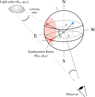
Figure 11.— Schematic view of the positional relationship between the southeastern knots and the light-echo.

Now we consider the relationship between the HVFs seen in the light echo spectrum and the SE knots by examining the positional relationship between them. Figure 11 shows a schematic view to guide the discussion. The plane of the sky lies in the plane defined by the NS-EW axes and we indicate a sphere with unit radius centered at the remnant’s center. We use a spherical polar coordinate system ($\theta$,$\phi$) as defined by the blue dot on the unit sphere. We assume a distance of 4.0 kpc.

The SE knots (indicated by the labeled red dot on the unit sphere) are slightly in front of the sky plane and are slightly south of the EW axis. According to Katsuda et al. (2010) the SE knots are located at angles of 97.5–107.5^∘ from north; we adopt the central value of $\theta_{\rm SK}=102.5^{\circ}$. We determine $\phi_{\rm SK}$ from the ratios of transverse and radial velocities, namely 0.55–0.58 (Si-rich knots) and 0.27–0.28 (Fe-rich knots). We assume the mean ratio ($\sim$0.42) which yields a value of $\phi_{\rm SK}\sim 23^{\circ}+270^{\circ}=293^{\circ}$.

The position on the sky of the light echo is about $3^{\circ}$ away from the center of Tycho’s SNR toward the NW and the polar angle is $\theta_{\rm LE}=62^{\circ}$; for our assumed distance of 4.0 kpc to Tycho’s SNR, the scattering angle is $65^{\circ}$. From these values (which we updated from the values in Krause et al., 2008), we determine that $\phi_{\rm LE}=270^{\circ}-(90^{\circ}-3^{\circ}-65^{\circ})=248^{\circ}$. Using spherical trigonometry, we determine that there is an angular separation of $\sim$$59^{\circ}$ between the centroid of the SE knots and the viewing direction of the light echo. The separation between the Fe-rich knots and the light echo is about the same $\sim$$59^{\circ}$.

There are systematic uncertainties on this result from the light echo (whose location with respect to the remnant depends on the assumed distance, since it must satisfy light-travel time arguments) and uncertainty on the radial velocities (as discussed above) and transverse velocities (whose main uncertainty is the assumed distance). Still we can set a robust lower limit on the angular separation between these based on the very accurately determined polar angles: $>$40^∘ (for the mean of the SE knots) and $>$45^∘ (for the Fe-rich knots).

Three-dimensional models suggest that large blobs (opening angle: $\sim$80^∘) or a thick torus (opening angle: $\sim$60^∘) can naturally explain observations of the HVFs (Tanaka et al., 2006). Although the angular separation between the knots and the direction to the light echo is similar to the sizes of these proposed structures, the unique feature of the SE quadrant is the presence there of Fe-rich knots, which are very localized. We therefore conclude that it is unlikely for the Fe-rich knots in the SE quadrant to be responsible for the HVF in the light echo spectrum.

Examining all six knots in the SE region (and ignoring systematic uncertainties in radial and transverse velocities) we find that they cover a full angular spread of $\Delta\theta\sim 35^{\circ}$ and $\Delta\phi\sim 40^{\circ}$. Yet how the knots are located is not random; there is a correlation between $\theta$ and $\phi$. Near the top of the feature (e.g., Knot1) $\phi\sim 299^{\circ}$, in the middle (e.g., Knot4) $\phi\sim 289^{\circ}$, and at the bottom (e.g., Knot6) $\phi\sim 260^{\circ}$. The knots appear to be distributed in a chain along the edge of the remnant and therefore form a distinct, fairly compact, and kinematically connected structure in Tycho’s SNR.

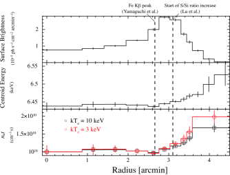
Figure 12.— Radial profiles of the Fe-K$\alpha$ surface brightness (top), centroid energy (middle), and ionization age (bottom) for Tycho’s SNR. The bottom panel is the result of spectral analysis using a vnei plus srcut model assuming fixed temperatures of 3 keV (red) and 10 keV (black) across the radial range shown. Dashed lines show the peak position of the Fe-K$\beta$ intensity (Yamaguchi et al., 2014) and the location where the S/Si line ratio begins to increase while moving out from the remnant’s center (Lu et al., 2015).

4.3. Fe Ionization State Increase at the Edge of Tycho’s SNR

The ejecta are heated as the reverse shock propagates from the outside of the remnant to the interior. Thus the ionization age of the shocked thermal plasma should vary with the time since the reverse shock passed (ignoring variations in the density of the ejecta). This is key information for our understanding of the heating processes at the reverse shock. Some recent X-ray imaging and spectroscopy studies have begun to shed light on this process. One example is the work by Yamaguchi et al. (2014) on the variation of the Fe ionization state near the reverse shock mentioned in the last section. In other work, Lu et al. (2015) found a systematic increase in the sulfur to silicon K$\alpha$ line flux ratio with radius through the outer edge of Tycho’s SNR, which they interpreted as a radial dependence of the ionization age.

In section 3.1, we found a strong increase in the Fe-K centroid energy also at the outer edge of Tycho’s SNR (see Figure 12). The line centroid energy (middle panel) increases by $\sim$90 eV over a radial distance of approximately 1^′. Carrying along in the same vein as the studies mentioned in the previous paragraph, we interpret this change as being due to a difference in the Fe ionization state and carried out spectral fits of the Fe-K$\alpha$ band spectra using the srcut (continuum) and vnei (thermal) models in XSPEC. The temperature of the vnei model was fixed at values of 3 keV and 10 keV; we used the ionization age parameter ($n_{e}t$) to account for the observed changes in centroid energy. As before for the srcut model, we fixed the radio spectral index to $\alpha=-0.65$. Note that the scenario we investigate here is intended to be illustrative. A future, more definitive study would consider the time evolution of temperature and density for a realistic ejecta density profile.

We found a gradual, modest increase of the ionization age from $10^{10}$ cm^-3 s to $1.7\times 10^{10}$ cm^-3 s (10 keV) or $2.0\times 10^{10}$ cm^-3 s (3 keV) over radii of $\sim$2.8^′ to $\sim$3.8^′. The inner radius is close to the peak position of the Fe-K$\beta$ emission and also to where the S/Si line ratio begins to increase moving out. The difference in Fe ionization age over the outer edge of Tycho’s SNR is $\Delta n_{e}t\sim(0.7-1.0)\times 10^{10}\,{\rm cm^{-3}s}\sim(220-320)(n_{e}/{\rm 1\,cm^{-3}})$ yr. This is a plausible range given the known age of Tycho’s SNR (440 yr); additionally the ionization timescale profile from the one-dimensional models of Tycho’s SNR (Badenes et al., 2006) show a strong radial gradient reaching values of $n_{e}t\sim 2\times 10^{10}\,{\rm cm^{-3}s}$ at the edge of the ejecta, while the electron temperature remains relatively flat at a value of $\sim$3 keV. However the radial region over which we see this variation is exactly where 1D models fail, i.e., where the Rayleigh-Taylor instability dominates the structure of the remnant. Understanding the thermodynamic evolution of the plasma in this region will allow us to better understand and model this important region.

5. Conclusions

In this paper we have carried out a detailed analysis of the deep Chandra ACIS-I observation ($\sim$734 ks in total exposure) of Tycho’s SNR. We have presented measurements of ejecta velocities and have investigated the heating processes in the ejecta. Our results can be summarized as follows.

1. We investigated the radial dependence of the Si-He$\alpha$, S-He$\alpha$, and Fe K$\alpha$ line intensity, line centroid, and line width and obtained results consistent with previous work. Chandra’s exceptional angular resolution allowed us to discover several new features in the radial profiles, including radial energy centroid shifts, a deep minimum in the line width profile for all species at a radius of $\sim$3.4^′, and a gradual increase in the Fe line centroid beyond radii of $\sim$3^′. From the line width profile we determined the expansion velocity of the Si-rich ejecta shell to be $5010\pm 340$ km s^-1 and, with the published proper motion of the Si-shell, obtained a distance measurement to Tycho’s SNR of $4.0\pm 0.3~{}^{+1.0}_{-0.7}$ kpc. Although this is fully consistent with the previous Suzaku result, it is subject to fewer systematic uncertainties.

2. The Si-He$\alpha$ line from Tycho’s SNR shows large ($\sim$60 eV) energy centroid shifts across the image with the largest range appearing near the center of the remnant. The distribution of centroid shifts is structured on scales ranging from arcseconds to arcminutes, which agrees qualitatively with the highly structured intensity distribution. Structure in the energy centroid image can be matched to features in the line centroid radial profile. We argue that these structures are due largely to differences in the intrinsic intensity of the approaching and receding hemispheres of the SNR.

3. We perform detailed spectral fits on 27 blobs using nonequiliubrium ionization thermal plasma models. We succeed in separating these features cleanly into redshifted, blueshifted, and low velocity clumps of ejecta. The determination of velocities is shown to be robust with respect to other spectral fit parameters that can influence line centroids, such as the ionization age parameter. For a subset of the most rapidly moving blobs we perform joint fits with the ACIS-S data in order to establish the level of systematic velocity uncertainty: $\sim$500–2,000 km s^-1 where the ACIS-S spectra tend to be more redshifted than ACIS-I. Using a local background for each blob tends to increase fitted velocities by approximately 1000–2000 km s^-1. We conclude after considering these factors that the velocities of the redshifted and blueshifted blobs are $\lesssim 7,800$ km s^-1 and $\lesssim 5,000$ km s^-1, respectively.

4. We conclude based on geometric considerations that the unusual Fe-rich knots in the southeastern quadrant are not likely to be responsible for the high velocity Ca II absorption features seen in the light echo spectrum. And if this exceptional set of knots is not responsible, then perhaps the origin of the HVF may be due to one of the more numerous, compact Si-rich knots that lie closer to the light echo direction. Future spectral and kinematic studies of the knots in this direction may yield important clues to the nature of the HVF in SN Ia spectra. A major step forward would be to obtain a light echo spectrum from a region off toward the SE of Tycho’s SNR (such as the fields 4523, 4821, and 5717 in Rest et al., 2008) that may provide a more direct view of the SE Fe-rich knots during the explosion.

5. We also note the detection of Cr K$\alpha$ line emission from 4 out of the 6 SE knots analyzed. Cr is also detected in most of the spectra from the radial profiles (at least out to Sky9). A careful study of the relative abundances of the Fe-group elements in the SE Fe-rich knots versus the rest of the remnant should in principle yield information about the explosion Si-burning processes in both regions.

6. Finally, we found that the Fe-K$\alpha$ energy centroid showed a gradual increase beyond the radius of the peak intensity. We interpreted this as a difference in the elapsed ionization time by an amount $\Delta n_{e}t\sim(220-320)(n_{e}/{\rm 1\,cm^{-3}})$ cm^-3 yr since the material was shock heated. The region over which we see this happening is the region where Rayleigh-Taylor fingers of ejecta extend out into the forward shock region. Studying this region in more detail will yield useful information on this process.

This work was initiated in preparation for observations of Tycho’s SNR with the Hitomi (ASTRO-H) satellite, which was sadly lost in March 2016. Our work with the Chandra ACIS detectors shows the richness of the science that can be extracted from the kinematics of SNRs. There is still much that Chandra can do in this area. The Chandra High Energy Transmission Gratings have been used to extract useful information on the kinematics of compact features in the extended remnants Cas A (Lazendic, Dewey, Schulz, & Canizares, 2006) and G292.0+1.8 (Bhalerao et al., 2015) and an observation of Kepler’s SNR (PI: Sangwook Park) with a similar goal was observed in 2016 July. Hopefully more remnants will be observed in coming cycles.

.1. Separate Radial Dependence of the Red- and Blueshifted Components of the Expanding Shell

In section 3.4, we showed that compact red- and blueshifted blobs could be identified thanks to Chandra’s high angular resolution. We also know that the radial profile of line width shows a gradual decline from a high value at the center (e.g., Furuzawa et al., 2009; Hayato et al., 2010), consistent with the scenario that we are seeing the combination of two different velocity components of an expanding shell. We now describe an additional analysis, that used Chandra’s high resolution in a different way, to separate the two shell components and provide additional confidence for the expanding shell scenario.

For each radial region we generated the distribution of Si-He$\alpha$ line centroid energies (Figure 13, left panel) from the centroid map (Figure 4, left panel). From this we calculated the mean photon energy and standard deviation of the distribution. Two spectra were extracted for each radial region: one for all pixels with energy centroids more than 1 standard deviation above the mean (the blueshifted spectrum) and the other for all pixels with centroids more than 1 standard deviation below the mean (the redshifted spectrum). Then we conducted spectral fitting (using the same spectral model as in § 3.1) for each pair of spectra from each region to obtain the centroid energies for each component. Figure 13 (right panel) shows the radial dependence of the Si-He$\alpha$ centroid energy for these two components. The general shapes of these two curves is consistent with the projection of each hemisphere (receding and approaching).

We approximate the projection effect with a pair of simple cosine functions (Figure 13 right). The curves are not a fit to the data. We took the values of the mean energy and standard deviation (1.856 keV and 10 eV) from the Sky8 region (the region closest to the edge of the Si shell) and added to these the cosine function for a shell of radus 3.4^′ and peak velocity of 4200 km s^-1. The data points show a similar trend, but seem to prefer a lower shell velocity. This is to be expected since the red- and blueshifted lines are broad (see Figure 3, top panel) and so the higher velocity pixels are diluted by the more numerous lower velocity ones. We also see the effect of the shell patchiness in the central radial bin. Our analysis here confirms that this region includes much more redshifted than blueshifted emission.

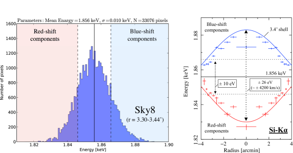
Figure 13.— Left: the histogram of mean photon energies from the Sky8 region (between radii of 3.30^′–3.44^′). Right: the radial dependence of the Si-He$\alpha$ centroid energies of the red- and blueshifted shell components. The blue and red solid lines show a cosine functions which approximatges the 3.4^′ shell expansion. This figure is symmetric for positive and negative radius.

References

- Anders & Grevesse (1989) Anders, E., & Grevesse, N. 1989, Geochim. Cosmochim. Acta, 53, 197
- Audard et al. (2001) Audard, M., Behar, E., Güdel, M., et al. 2001, A&A, 365, L329
- Baade (1945) Baade, W. 1945, ApJ, 102, 309
- Badenes et al. (2006) Badenes, C., Borkowski, K. J., Hughes, J. P., Hwang, U., & Bravo, E. 2006, ApJ, 645, 1373
- Bautz et al. (1998) Bautz, M. W., et al. 1998, Proc. SPIE, 3444, 210
- Benetti et al. (2005) Benetti, S., Cappellaro, E., Mazzali, P. A., et al. 2005, ApJ, 623, 1011
- Bhalerao et al. (2015) Bhalerao, J., Park, S., Dewey, D., Hughes, J. P., Mori, K., & Lee, J.-J. 2015, ApJ, 800, 65
- Brickhouse et al. (2000) Brickhouse, N. S., Dupree, A. K., Edgar, R. J., et al. 2000, ApJ, 530, 387
- Broersen et al. (2013) Broersen, S., Vink, J., Miceli, M., et al. 2013, A&A, 552, A9
- Cappellari & Copin (2003) Cappellari, M., & Copin, Y. 2003, MNRAS, 342, 345
- Cargill & Papadopoulos (1988) Cargill, P. J., & Papadopoulos, K. 1988, ApJ, 329, L29
- Childress et al. (2014) Childress, M. J., Filippenko, A. V., Ganeshalingam, M., & Schmidt, B. P. 2014, MNRAS, 437, 338
- Decourchelle et al. (2001) Decourchelle, A., Sauvageot, J. L., Audard, M., et al. 2001, A&A, 365, L218
- Diehl & Statler (2006) Diehl, S., & Statler, T. S. 2006, MNRAS, 368, 497
- Eriksen et al. (2011) Eriksen, K. A., Hughes, J. P., Badenes, C., et al. 2011, ApJ, 728, L28
- Furuzawa et al. (2009) Furuzawa, A., Ueno, D., Hayato, A., et al. 2009, ApJ, 693, L61
- Garmire et al. (1992) Garmire, G. P., et al. 1992, AIAA Space Program and Technologies Conference: The AXAF CCD Imaging Spectrometer (New York: AIAA)
- Gu et al. (2007) Gu, M. F., Chen, H., Brown, G. V., Beiersdorfer, P., & Kahn, S. M. 2007, ApJ, 670, 1504
- Hayato et al. (2010) Hayato, A., Yamaguchi, H., Tamagawa, T., et al. 2010, ApJ, 725, 894
- Hughes et al. (2014) Hughes, J. P., Safi-Harb, S., Bamba, A., et al. 2014, arXiv:1412.1169
- Hughes (2000) Hughes, J. P. 2000, ApJ, 545, L53
- Hwang et al. (2002) Hwang, U., Decourchelle, A., Holt, S. S., & Petre, R. 2002, ApJ, 581, 1101
- Ishisaki et al. (2007) Ishisaki, Y., Maeda, Y., Fujimoto, R., et al. 2007, PASJ, 59, 113
- Jordan et al. (2008) Jordan, G. C., IV, Fisher, R. T., Townsley, D. M., Calder, A. C., Graziani, C., Asida, S., Lamb, D. Q., & Truran, J. W. 2008, ApJ, 681, 1448-1457
- Kasen et al. (2003) Kasen, D., Nugent, P., Wang, L., et al. 2003, ApJ, 593, 788
- Katsuda et al. (2010) Katsuda, S., Petre, R., Hughes, J. P., et al. 2010, ApJ, 709, 1387
- Katsuda et al. (2015) Katsuda, S., Mori, K., Maeda, K., et al. 2015, ApJ, 808, 49
- Kothes et al. (2006) Kothes, R., Fedotov, K., Foster, T. J., & Uyanıker, B. 2006, A&A, 457, 1081
- Koyama et al. (2007) Koyama, K., et al. 2007, PASJ, 59, S23
- Krause et al. (2008) Krause, O., Tanaka, M., Usuda, T., et al. 2008, Nature, 456, 617
- Kuhlen et al. (2006) Kuhlen, M., Woosley, S. E., & Glatzmaier, G. A. 2006, ApJ, 640, 407
- Lazendic, Dewey, Schulz, & Canizares (2006) Lazendic, J. S., Dewey, D., Schulz, N. S., & Canizares, C. R. 2006, ApJ, 651, 250
- Long et al. (2014) Long, K. S., Bamba, A., Aharonian, F., et al. 2014, arXiv:1412.1166
- Lu et al. (2015) Lu, F. J., Ge, M. Y., Zheng, S. J., et al. 2015, ApJ, 805, 142
- Maeda et al. (2010) Maeda, K., Benetti, S., Stritzinger, M., et al. 2010, Nature, 466, 82
- Maeda et al. (2010) Maeda, K., Röpke, F. K., Fink, M., Hillebrandt, W., Travaglio, C., & Thielemann, F.-K. 2010, ApJ, 712, 624
- Mazzali et al. (2005) Mazzali, P. A., Benetti, S., Altavilla, G., et al. 2005, ApJ, 623, L37
- McKee (1974) McKee, C. F. 1974, ApJ, 188, 335
- Murtagh & Heck (1987) Murtagh, F., & Heck, A. 1987, Multivariate Data Analysis (Dordrecht: D. Reidel)
- Perlmutter et al. (1999) Perlmutter, S., Aldering, G., Goldhaber, G., et al. 1999, ApJ, 517, 565
- Phillips et al. (1999) Phillips, M. M., Lira, P., Suntzeff, N. B., et al. 1999, AJ, 118, 1766
- Plewa, Calder, & Lamb (2004) Plewa, T., Calder, A. C., & Lamb, D. Q. 2004, ApJ, 612, L37 Haberl, F., Dewey, D., et al. 2008, Proc. SPIE, 7011, 70112E
- Plucinsky et al. (2016) Plucinsky, P. P., Beardmore, A. P., Foster, A., et al. 2016, arXiv:1607.03069
- Rest et al. (2008) Rest, A., Welch, D. L., Suntzeff, N. B., et al. 2008, ApJ, 681, L81
- Riess et al. (1998) Riess, A. G., Filippenko, A. V., Challis, P., et al. 1998, AJ, 116, 1009
- Röpke, Woosley, & Hillebrandt (2007) Röpke, F. K., Woosley, S. E., & Hillebrandt, W. 2007, ApJ, 660, 1344
- Ruiz-Lapuente et al. (2004) Ruiz-Lapuente, P., Comeron, F., Méndez, J., et al. 2004, Nature, 431, 1069
- Seward et al. (1983) Seward, F., Gorenstein, P., & Tucker, W. 1983, ApJ, 266, 287
- Shklovsky (1968) Shklovsky, J. S. 1968, Supernovae, Interscience Monographs and Texts in Physics and Astronomy, London: Wiley
- Slane et al. (2014) Slane, P., Lee, S.-H., Ellison, D. C., et al. 2014, ApJ, 783, 33
- Spitzer (1978) Spitzer, Jr., L. 1978, Physical Process in the Interstellar Medium (New York: John Wiley & Sons)
- Takahashi et al. (2014) Takahashi, T., Mitsuda, K., Kelley, R., et al. 2014, Proc. SPIE, 9144, 914425
- Tanaka et al. (2006) Tanaka, M., Mazzali, P. A., Maeda, K., & Nomoto, K. 2006, ApJ, 645, 470
- Uchida et al. (2013) Uchida, H., Yamaguchi, H., & Koyama, K. 2013, ApJ, 771, 56
- Uchiyama et al. (2009) Uchiyama, H., Ozawa, M., Matsumoto, H., et al. 2009, PASJ, 61, S9
- Vancura et al. (1995) Vancura, O., Gorenstein, P., & Hughes, J. P. 1995, ApJ, 441, 680
- Vink et al. (2003) Vink, J., Laming, J. M., Gu, M. F., Rasmussen, A., & Kaastra, J. S. 2003, ApJ, 587, L31
- Vink et al. (2010) Vink, J., Yamazaki, R., Helder, E. A., & Schure, K. M. 2010, ApJ, 722, 1727
- Wang et al. (2003) Wang, L., Baade, D., Höflich, P., et al. 2003, ApJ, 591, 1110
- Warren et al. (2005) Warren, J. S., Hughes, J. P., Badenes, C., et al. 2005, ApJ, 634, 376
- Warren & Blondin (2013) Warren, D. C., & Blondin, J. M. 2013, MNRAS, 429, 3099
- Woosley et al. (2004) Woosley, S. E., Wunsch, S., & Kuhlen, M. 2004, ApJ, 607, 921
- Woosley (2007) Woosley, S. E. 2007, ApJ, 668, 1109
- Yamaguchi et al. (2008) Yamaguchi, H., Koyama, K., Katsuda, S., et al. 2008, PASJ, 60, S141
- Yamaguchi et al. (2014) Yamaguchi, H., Eriksen, K. A., Badenes, C., et al. 2014, ApJ, 780, 136