Three X-ray Flares Near Primary Eclipse of the RS CVn Binary XY UMa

Abstract

We report on an archival X-ray observation of the eclipsing RS CVn binary XY UMa ($\rm P_{orb}\approx$ 0.48d). In two Chandra ACIS observations spanning 200 ks and almost five orbital periods, three flares occurred. We find no evidence for eclipses in the X-ray flux. The flares took place around times of primary eclipse, with one flare occurring shortly ($<0.125\rm P_{orb}$) after a primary eclipse, and the other two happening shortly ($<0.05\rm P_{orb}$) before a primary eclipse. Two flares occurred within roughly one orbital period ($\Delta\phi\approx 1.024\rm P_{orb}$) of each other. We analyze the light curve and spectra of the system, and investigate coronal length scales both during quiescence and during flares, as well as the timing of the flares. We explore the possibility that the flares are orbit-induced by introducing a small orbital eccentricity, which is quite challenging for this close binary.

1 Introduction

X-ray studies of short orbital period systems provide the opportunity to investigate coronal structures by investigating the phase dependence of emission, with the advantage that multiple orbital periods are often accessible. Due to the effect of tidal locking and the increase of stellar magnetic activity with decreasing rotation period (Reiners et al. 2014), some short orbital period systems display enhanced magnetic activity. However, the phenomenon of supersaturation of the X-ray emission can also occur, leading to a decrease in the level of observed magnetic activity (Wright et al. 2011). Eclipsing systems additionally allow for constraints on the extent of X-ray emitting material above the stellar photosphere. Previous X-ray studies of short-period systems have found a lack of strong X-ray eclipses, with suggestions of high latitude, compact coronae, from systems as short period as 0.27 d (contact binary systems VW Ceph and 44 iBoo; Huenemoerder et al. 2006; Brickhouse et al. 2001 respectively ). A recent study of the M dwarf eclipsing binary YY Gem (Hussain et al. 2012), a P${}_{\rm rot}=P_{\rm orb}=$0.81 d, M1V+M1V binary, found that there were no strong X-ray eclipses, and both components were active. Other studies have suggested a causal connection between the timing of flares and periastron passage in close binaries (Massi et al. 2002, 2008; Getman et al. 2011), with the interpretation that of interacting magnetospheres of two systems. These stellar systems can also provide a context in which to place star-planet interactions with close-in, magnetized exoplanets (Rubenstein & Schaefer 2000).

RS Canum Venaticorum systems (RS CVns hereafter, Hall 1976, 1989) are close but detached binaries, typically with a G/K giant or subgiant + a late-type main sequence/subgiant companion. Regular RS CVns have orbital periods between 1 and 14 days, while systems with short periods less than one day can also exist. Tidal locking enhances chromospheric and coronal emission, making RS CVns among the most magnetically active late type stellar systems (see the introduction of Osten & Brown 1999). Since its discovery in 1955, XY UMa has been one of the most intensively observed RS CVn binaries. It has the fifth shortest orbital period ($\approx$0.47899d) according to the RS CVn binary catalog (Dryomova et al. 2005), which means both of its two companions, G2-3V+K4-5V (Strassmeier et al. 1993; Pojmanski & Udalski 1997), should have become tidally locked (Zahn 1977; Tassoul 1988; Tassoul & Tassoul 1992; Abt 2006; Meibom et al. 2006; Mazeh 2008). As described in Pribulla et al. (2001), there are two different distances, one based on Hipparcos astrometric data (66$\pm$6 pc) and the other based on the absolute magnitudes of the two companions (86$\pm$5 pc). Here, we adopt the second value because of Hipparcos’ short-term coverage and the possible perturbation on the astrometry by a third object. The binary parameters are $\rm{R_{1}}$=1.16 $\rm R_{\odot}$, $\rm{R_{2}}$=0.63 $\rm R_{\odot}$, the semi-major axis a=3.107 $\rm R_{\odot}$ and the orbital inclination i=80.86^∘, while Erdem & Gudur (1998) derive the orbital inclination of 76^∘, relative to an edge-on system of 90^∘.

Hilditch & Bell (1994) showed XY UMa had substantial star spot activity based on 1189 V-band photometric observations in 1992 October. They claimed the existence of a dark zone encircled the primary star between $\pm 15^{\circ}$ in latitude and spot accumulation at the inner hemisphere of the primary. Also based on substantial optical photometric data, Collier Cameron & Hilditch (1997) and Lister et al. (2001) used eclipse mapping to map the spot distribution. Their results are consistent with Hilditch & Bell (1994) and showed the spot evolution in few days to one week. Hilditch & Collier Cameron (1995) interpreted long-term photometric variations of XY UMa as originating partly in a polar spot on the primary, which dominates the optical photometric variability.

Although XY UMa is magnetically active and has long term photometric observations in the past several decades, relatively few optical flares have been seen (Jeffries & Bedford 1990). Only two flare-like events were reported in optical band. Zeilik et al. (1983) discovered one between phases 0.54 and 0.62 at UBV bands, while the other (Özeren et al. 2001), derived from the excess emission in $\rm H_{\alpha}$, occurred between phases 0.6 and 0.8. The lack of optical flare detections could be result of flare-induced brightenings being relatively small compared with XY UMa’s overall optical brightness. XY UMa is also X-ray bright. It was observed by EXOSAT for a continuous 14.5 hours in 1986. A moderately higher count rate between phases 1.41 and 1.47 for about 1.5 ks was interpreted as a flare event by Jeffries & Bedford (1990), but it was not mentioned by a previous analysis (Bedford et al. 1990) of the same data. XY UMa was also observed by ROSAT for a total 37 ks in 1992. An enhanced count rate was detected at phase 0.5 exactly in the folded light curve of different observations (Jeffries 1998). In general, three flares out of the four noted in the literature occur near the secondary eclipse.

The paper is organized as follows: §2 describes the observations and data reduction; §3 describes what we can derive about the coronal length scales in both quiescence and during flares, as well as what we can say about the timing of the X-ray flares. §4 has a discussion of the results and §5 concludes.

2 Chandra Observation And Data Reduction

As Table.1 shows, XY UMa was observed by Chandra twice, with observations separated by five days in 2001 April. The two observations were similarly configured except for the exposure time. The original purpose of the observations was an X-ray cluster survey. In processing all of the publicly available ACIS data while searching for flare-like events, we discovered three flares from XY UMa.

The large off-axis angle of XY UMa introduces several technical problems. One concern is whether XY UMa has dithered off the detector. The standard dither pattern of the Chandra telescope is 16$\arcsec$, but the position of XY UMa is about 1$\arcmin$ away from the edge of the detector. The large off-axis angle combined with the spokes (Figure 4.14 of Chandra’s POG 18) in the image may attenuate the count rate of XY UMa, but the profile of the light curve can be recovered. We also assess whether XY UMa is affected by pileup because of its brightness. The script $pileup\_map$ of CIAO 4.7 returns 0.067 (count/event island/frame time) near the centroid of XY UMa(ObsID=2227), which corresponds to $<$ 5% pileup fraction in the 3x3 pixel cell of the most brightest region, where there are only about 3000 counts.

Table 1: Chandra Observations of XY UMa

Instrument	Date	ID	Exposure Time	Countsa	Off-axis angle	Sizeb
ACIS-I	2001 Apr 24	2452	76 ks(1.84$\rm P_{orb}$)	19579/18295	11.23$\arcmin$	12.1$\arcsec$x10.0$\arcsec$
ACIS-I	2001 Apr 29	2227	124 ks(3.00$\rm P_{orb}$)	46302/43302	11.32$\arcmin$	12.0$\arcsec$x10.0$\arcsec$

^a0.3-10 keV photons in the 3$\sigma$ elliptical region by $wavdetect$ and a 10$\arcsec$ radius circle respectively
^baxis length of the 3$\sigma$ elliptical region

2.1 The Phase

Because our analysis makes use of the times of primary and secondary eclipse during the X-ray observations, we use an optical light curve from Heckert (2012). This is the optical observation closest to the time of the Chandra observations we can find, taken just 20 days after the Chandra observations. Lister et al. (2001) showed the zero point of the ephemeris in 2000 has about half an orbital period shift compared with the zero point in 1999. This means it is necessary to adopt an observation close in time to keep the phase coherence. Hence, the phase uncertainties here are not from the ephemeris (Lister et al. 2001), but mainly from the orbital period ($<1\times 10^{-5}$ d, Chochol et al. 1998; Pribulla et al. 2001) and the timing precision of every V band photometric point ($\approx 1\times 10^{-4}$ d) given by Heckert (2012). The combined temporal uncertainty of each point in the V band light curve is less than 10 minutes.

2.2 X-ray Light Curves

Data reduction began with reprocessing the level 2 data for both observations by $chandra\_repro$ to ensure consistent calibration updates and the newest software are applied. Then, X-ray photons between 0.3-10 keV were extracted from the $3\sigma$ elliptical region derived by $wavdetect$, the workhorse of CIAO for source detection. If we use a 10$\arcsec$ radius circle as the source region, the X-ray counts do not vary much. Because the optical data described in §2.1 is in HJD, the X-ray timing data are also converted to Heliocentric Julian Day (HJD) according to web pages. The HJD correction is no more than 1 minute compared with Julian date. We adjust the time bin scale and find a 200 s time binning reduces uncertainties in each light curve bin while retaining information about any temporal variations.

Figure.1 shows the X-ray light curves, along with the hardness ratio, using the 200 s binning. The hardness ratio (HD ratio) is defined as (h-s)/(h+s), in which $s$ is the number of counts in a soft band (0.3 to 2 keV), while $h$ is the number of counts in a hard band extending from 2 to 10 keV. A roughly synchronous evolution can be seen compared with X-ray light curves. Figure.1 also overplots the V band photometry, to illustrate the times of primary and secondary eclipse. As Figure.1 shows, two large flares (f1 and f2 hereafter) occurred shortly before two primary eclipses in the second observation, while a smaller flare (f3 hereafter) occurred in the first observation five days earlier. The peak count rates of f1, f2 and f3 increase with a factor of about 4.2, 2.6 and 2.4 respectively compared with the base level (between 50 counts/bin and 75 counts/bin of the light curve selected by eye. We note key times in the light curve: b1 and s1 are the approximate beginning and ending, respectively, of f1, b2 and s2 are the corresponding quantities for f2. The peaks of f1 and f2 are denoted p1 and p2, respectively, and are the locations of local maxima in the light curves of f2 and f2. The location of optical primary eclipses are termed e0, e1, and e2, and are also marked in the light curve.

Because of the asymmetrical profiles and the relatively sparse counts near the flare peaks, we directly adopt points with the biggest counts, p1 and p2, as flare peaks. The separation between the peak of f1 and its corresponding primary eclipse is about 71.2 minutes, and for f2, it is about 54.2 minutes. The difference (17min $\approx 0.024\rm P_{orb}$) could be bigger or smaller depending on where the flare peaks and where primary eclipses are exactly. Using a Possion error for every time bin and the method of least squares, assuming an exponential $y=a\times e^{-t/\tau}+b$ decay, we obtain an e-folding decay time $\tau$=1433$\pm$249s ($\chi^{2}$=1.9, dof=31) for [p1, s1], while $\tau$=3732$\pm$1236s ($\chi^{2}$=1.4, dof=26) for [p2, s2]. The decay continues between s1 and b2, but the exponential fit is poor because of fluctuations after s1.

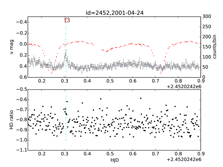
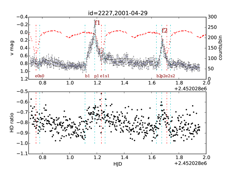
Figure 1: X-ray light curves from the two Chandra observations

In the two upper panels, the blue points are from the X-ray data, while the red points are from real optical observations which have a 20 day offset. The hardness ratios are in the lower panels. Critical timing points selected by eye and primary eclipses are marked by cyan and red dashed lines respectively in all panels.

2.3 X-ray Spectra

The X-ray spectrum of coronally active stars is well-described by a collisionally ionized plasma, and we use the absorbed ($xswabs$) APEC model (Smith et al. 2001) implementation in Sherpa to fit each spectrum. Time-resolved X-ray spectra were extracted using the light curve time intervals noted in Figure.1. The [p1,s1] and [s1,b2] temporal intervals were subdivided into two and three equal parts, respectively, to get some resolution, and spectra were extracted from each sub-interval. Source and background spectra were created by $specextract$ and fit by an absorbed two-temperature APEC model. We freeze the redshift in APEC to be zero, leave all other parameters free, and use the Sherpa $moncar$ (the Monte Carlo optimization method) to search for the best model parameters.

The value of N_H is not constrained, but N_H obtained are all near zero. We settled on using two temperature components to describe the spectra: a one-temperature APEC model produced large $\chi^{2}$ values, indicating an inadequacy of the spectral fits. Spectra corresponding to non-flare temporal bins could also be described by a four-temperature APEC model, but the improvement is not enough. The non-flare parts are relatively poorly fit. Results are shown in Table.2.

The spectra of f1 ([b1,s1]) and f2 ([b2,s2]) are shown in Figure.2. Both have a 2.1 keV instrumental absorption edge (Table 9.4 of Chandra’s POG 18; Moran et al. 2005), which also indicates photon pileup can be ignored. Taking the integrated flux from the segments within [b1,s1] and [b2,s2] in Table.2 and multiplying by the integration times and assumed distance of 86 pc, the radiated energies in the 0.3-10 keV bandpass for f1 and f2 are $1.1\times 10^{35}$ erg and $5.5\times 10^{34}$ erg, respectively.

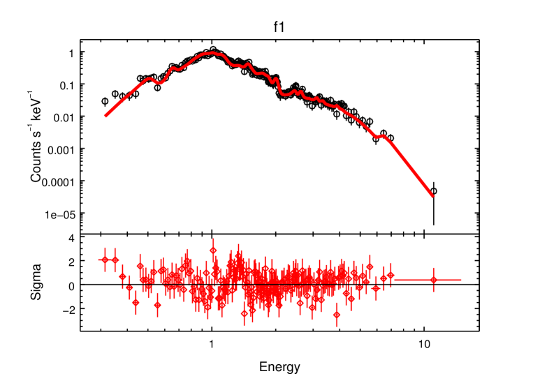
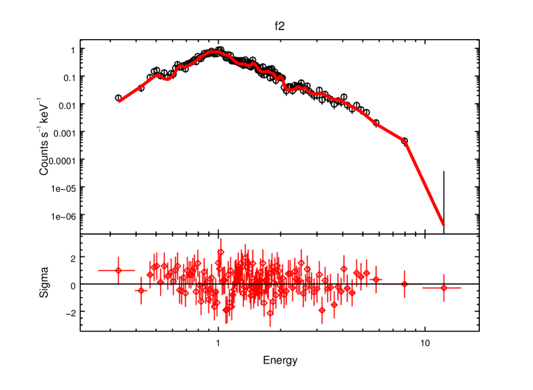
Figure 2: An absorbed-2T fit for f1 and f2. The high temperature part evolves, while the low temperature part sustains at about 1 keV.

3 Analysis

3.1 Quiescent Coronal Length Scales

Despite the fact that the X-ray observations span multiple binary eclipses, Figure.1 reveals that there is no apparent diminution of the X-ray flux during these events. The Volume Emission Measures (VEMs) reported in Table.2 outside of flares provide a constraint on emitting volumes and hence length scales, for assumptions about the coronal electron density. The volume emission measure in Table.2 is $VEM=n_{e}n_{H}dV$, with $n_{e}$ the coronal electron density, $n_{H}$ the number density of Hydrogen, and $dV$ the emitting volume. For a fully ionized plasma, $n_{H}/n_{e}=$0.8. The interval between 0 and b1 in Table.2 should occur during a primary eclipse, according to Figure.1, and we use the emission measures reported to investigate physical length scales. Ness et al. (2004) examined coronal electron densities derived from density-sensitive X-ray line diagnostics, for a range of stellar activity levels. Densities derived from the Ne 9 triplet, formed at a temperature around 4 MK, ranged from $\log n_{e}$ (cm^-3)=10.5$-$12, and they found no conclusive trend of densities with activity level for the higher activity stars. As this temperature is closest to the lower of the two temperatures returned from our spectral fitting, we use the emission measure reported in Table.2 for the 0.92 keV plasma (0.92 keV$\approx$11 MK), which is $n_{e}n_{H}dV=$5.27$\times$10²⁷ cm^-3. Evaluating at the low and high ends of the electron densities found in Ness et al. (2004), the coronal volume ranges between 6.6$\times$10²⁸ cm³ and 6.6$\times$10³¹ cm³. This is consistent with the volume trends described in Osten et al. (2003).

If this volume is distributed homogeneously over the surface of one star, then the height of the coronal shell can be estimated from

$$V_{\rm cor}=4\pi R_{\star}^{2}h_{\rm cor}$$ (1)

where $V_{\rm cor}$ is the coronal emitting volume, R_⋆ is the stellar radius, and $h_{\rm cor}$ is the height of a spherically symmetric X-ray-emitting region. Evaluating separately for each star, we find

$$h_{\rm cor,1} = 8\times 10^{5}-8\times 10^{8}\;\;\;cm$$ (2)

$$h_{\rm cor,2} = 2.7\times 10^{6}-2.7\times 10^{9}\;\;\;cm$$ (3)

for the primary and secondary, respectively, with $R_{1}=1.16R_{\odot}$ for the primary and $R_{2}=0.63R_{\odot}$ for the secondary. These sizes are very small compared to the binary separation (3.1 R_⊙ = 2.2$\times$10¹¹ cm), and would suggest that the X-ray-emitting material would be eclipsed as well. In order for this not to be the case, the coronal material should be at a high latitude which is always visible.

The geometry of the system provides another constraint on the coronal length scales during quiescence. Assuming that the orbital and rotational axes are aligned, the constraint on the orbital inclination of $\i=14^{\circ}$ from Erdem & Gudur (1998) suggests that an emitting region on the surface of either star would need to be located between $0$ and $14$ ^∘ co-latitude (i.e., at the visible pole or up to 14^∘ away in latitude). For an extended structure, we use the formalism described in Lim et al. (1994), using the quantity $\xi$,

$$\xi=\sin\theta\sin i\cos\phi+\cos\theta\cos i$$ (4)

where $\theta$ is the co-latitude of the emitting region, $\phi$ is the longitude, and $\i$ is the inclination (with a 90^∘ offset in the orbital inclination used above). An emitting region above the surface is visible as long as $\xi>0$ and the relation

$$\left(1+\frac{h}{R_{\star}}\right)\sqrt{(1-\xi^{2})}>1$$ (5)

holds. We evaluated these conditions for each star to determine the minimum height required to be visible at all longitudes, and found that a relative height of 0.03 R_⋆ was sufficient. For the primary, this works out to $\approx$2.5$\times$10⁹ cm, and for the secondary it is 1.4$\times$10⁹ cm.

3.2 Flaring Length Scale

The light curve and spectral evolution of flaring plasma hold information about the flaring coronal length scales, once assumptions about the release of energy and geometry are made. Most often, analyses of the decay phase of stellar coronal flares are used to reveal a loop semi-length using the method of Reale et al. (1997). Reale (2007) gives an empirical relation based on max(temperature) $\rm{T_{0}}$, max(emission measure), the time ($t_{M,3}$) at which max(EM) occurs and the temperature $\rm{T_{M}}$ when max(EM) occurs. In light of the poor statistics given by our spectral fitting of sub-intervals of the decay phase of f1, we use this alternate method to estimate the size of a single flaring loop. We evenly divide the decay phase of [p1,s1] and [s1,b2] respectively, and have five temperature bins. As Table.2 shows, emission measure drops sharply after [p1,s1]a (@9.42 ks), while the temperature sustains around 3.2 keV. Using Equation(12) of Reale (2007),

$$\rm{L_{9}}\approx 3{\Psi}^{2}\sqrt{\rm{T_{0,7}}}t_{M,3}$$ (6)

where $\rm{T_{0}}$ is the maximum temperature attained during the flare, $\rm{T_{0,7}}$ is $\rm{T_{0}}$ in units of 10⁷K, $\rm{t_{M}}$ is the time at which the maximum emission measure occurs, $t_{M,3}$ is $\rm{t_{M}}$ in units of 1000 seconds, and $\Psi$ is $\frac{\rm{T_{0}}}{\rm{T_{M}}}$. Evaluating this for f1, we let $\rm{T_{0}}\approx T_{M}$=3.2 keV and $t_{M,3}$=(102+55)minutes=9420s, and get the loop half length $\rm{L}\approx 3\times{(\frac{3.2}{3.2})}^{2}\times\sqrt{3.2\times 1.16}\times 9.42\times 10^{9}$ cm=0.78 $\rm R_{\odot}$. Then the loop height is 0.50 $\rm R_{\odot}$ assuming a vertical and circular loop. Hence, if it is one single loop, it is not long enough to anchor on the two companions simultaneously, but the loop height is a significant fraction of the separation between the two companions, and thus there could be magnetosphere interaction in between.

Table 2: APEC Fit

Phase	Duration	APEC.2T	$\chi^{2}$(dof)	Fluxa	Luminosityb	EM
………	(minute)	(keV)	………	…	($\rm{10^{30}\ erg\ s^{-1}}$)	($\rm{10^{53}}cm^{-3}$,$\rm{10^{52}\,cm^{-3}}$)
[0, b1]	576	$2.62^{+0.29}_{-0.09},0.92^{+0.01}_{-0.01}$	2.4(171)	4.4	3.9	$1.42^{+0.04}_{-0.04},5.27^{+0.21}_{-0.21}$
[b1, p1]	102	$2.98^{+0.18}_{-0.18},0.97^{+0.03}_{-0.03}$	0.9(127)	9.7	8.6	$3.83^{+0.14}_{-0.14},7.17^{+0.60}_{-0.61}$
[p1, s1]a	55	$3.20^{+0.26}_{-0.24},1.00^{+0.03}_{-0.03}$	0.9(102)	11.1	9.8	$4.25^{+0.21}_{-0.21},8.77^{+0.90}_{-0.90}$
[p1, s1]b	55	$3.22^{+0.33}_{-0.30},1.00^{+0.03}_{-0.04}$	0.7(78)	7.4	6.5	$2.80^{+0.18}_{-0.18},6.20^{+0.79}_{-0.79}$
[s1, b2]a	180	$2.87^{+0.18}_{-0.17},0.98^{+0.02}_{-0.02}$	1.4(129)	5.8	5.1	$2.11^{+0.08}_{-0.08},5.61^{+0.37}_{-0.37}$
[s1, b2]b	180	$2.24^{+0.14}_{-0.12},0.92^{+0.03}_{-0.03}$	1.1(116)	4.9	4.3	$1.69^{+0.08}_{-0.08},5.43^{+0.42}_{-0.46}$
[s1, b2]c	180	$2.52^{+0.18}_{-0.18},0.94^{+0.03}_{-0.03}$	1.5(106)	4.4	3.9	$1.34^{+0.07}_{-0.07},5.64^{+0.40}_{-0.40}$
[b2, p2]	55	$3.57^{+0.54}_{-0.39},0.96^{+0.03}_{-0.04}$	0.8(72)	6.4	5.6	$2.13^{+0.15}_{-0.16},6.39^{+0.69}_{-0.69}$
[p2, s2]	93	$3.22^{+0.26}_{-0.24},0.97^{+0.02}_{-0.03}$	0.9(106)	7.3	6.4	$2.54^{+0.13}_{-0.13},7.17^{+0.60}_{-0.59}$
[s2, end]	309	$2.57^{+0.16}_{-0.15},0.93^{+0.02}_{-0.02}$	1.8(126)	3.7	3.3	$1.04^{+0.05}_{-0.05},5.30^{+0.28}_{-0.28}$
f1:[b1, s1]	212	$3.09^{+0.12}_{-0.12},0.98^{+0.02}_{-0.02}$	1.1(173)	9.7	8.6	$3.79^{+0.09}_{-0.09},7.47^{+0.41}_{-0.41}$
f2:[b2, s2]	148	$3.31^{+0.22}_{-0.19},0.97^{+0.02}_{-0.02}$	0.9(129)	7.0	6.2	$2.41^{+0.10}_{-0.10},7.00^{+0.44}_{-0.44}$

^aabsorbed flux between 0.3-10 keV in unit of $10^{-12}\rm{erg\,cm^{-2}\,s^{-1}}$
^bluminosity based on absorbed flux

3.3 Timing of the flares

RS CVns should flare more frequently than typical binaries in the X-ray band, due to their shorter orbital and hence rotational periods. However, it is difficult to assess how frequently a particular RS CVn binary flares since long term X-ray observations of any one system are lacking. Osten & Brown (1999) analyzed 12.2 Ms EUVE photometric data of 16 RS CVn binaries and partly answered this question. Of the dozens of flares, only a few had peak flare count rates increase by more than a factor of three compared to the non-flaring count rates. As noted in §2.2, the peaks of these flares are factors of 4.2, 2.6, and 2.4 above a non-flaring count rate, and the integrated energies derived in §2.3 also reveal these to be large releases of energy.

The energetic releases of these two flares are fairly large and should occur relatively rarely. Here we attempt to quantify this by extrapolating from what is known about flares on RS CVn systems as well as single stars. Audard et al. (2000) characterized the coronal flare frequency of active single G and K dwarfs as a function of the star’s X-ray luminosity,

$$N(>10^{32}erg)=1.9\times 10^{-27}L_{x}^{0.95}\rm{\ flares/day}$$ (7)

above a flare energy of 10³² erg, and we use this to estimate the number of flares which would be expected to occur on one of the stars in the XY UMa system, assuming that the flare frequency distribution for tidally locked binary systems is similar to that of single active stars. We compute $L_{x}$ using the values for quiescence in Table.2, and dividing the observed X-ray luminosity (3.9$\times$10³⁰ erg s^-1) equally between the two stars. Osten & Brown (1999) investigated the flare frequency versus energy distribution for the 16 RS CVn systems mentioned above, and characterized it by an index $\alpha$ near 1.6, where the differential number of flares occurs per unit time per unit energy as $dN/dE\propto E^{-\alpha}$. More recent investigations of flare frequency distributions for active stars have revealed a range of $\alpha$ going up to about 2.2 (Güdel 2007), and we consider this range here, as the precise flare frequency distribution for XY UMa is not known. Given the flare rate in Audard et al. (2000), the number of flares expected a critical level $E_{\rm crit}$ is,

$$N_{\rm expected}=N_{\rm tot}\left(\frac{E_{\rm crit}}{E_{\rm min}}\right)^{1-\alpha}$$ (8)

with $E_{\rm min}$=10³² erg, and $N_{\rm tot}=N(>10^{32}erg)\times\Delta t$ flares. For $\alpha=$1.6,1.8,2.0,2.2, and a critical flare energy of $1.1\times 10^{35}$ erg (the radiated energy of the f1 flare), we would expect 2.4,0.6,0.1,0.04 flares in the 1.44 days of the 29 April observation. Thus these flares are consistent or marginally consistent with the expected number of flares for the flatter distributions, but for the steeper distributions ($\alpha\geq$ 2) they are incompatible. At this point the large loop lengths coupled with particular timing of flares relative to primary eclipse are suggestive but not conclusive of magnetospheric interaction in this binary system.

4 Discussion

It is curious that two of the flares observed on XY UMa occurred within 0.05 P_orb of primary eclipses of the binary system. We have investigated via flare loop hydrodynamic modelling whether the flaring structures are large enough to enable interactions between the two stars in the binary system, given how close they are. The separation of the two stellar surfaces is only a few stellar radii, making it plausible that a flaring loop of height 0.5 $\rm R_{\odot}$ could possibly interact with a similarly sized loop on the other star of the binary system. The fact that the X-ray observations do not show any evidence of primary or secondary eclipses indicates fairly extended coronal structures. The flares themselves exhibit a fairly classic rise and decay light curve structure without evidence for eclipses of the flaring material.

The similar phases of the three sporadic flares near primary eclipse make XY UMa a stunted version of CF Tuc (Gunn et al. 1997). Also as an eclipsing RS CVn system, with a 2.78d orbit, CF Tuc shows a clear modulation with a radio-flux maximum at phase 0.5, which is caused by an active intra-binary region probably. V711 Tau shows a similar behaviour seen here, in that two nearly identical flares, which both increase by a factor of about two, are separated by $\approx\frac{2}{3}\rm P_{orb}$. The binary $\sigma^{2}$ CrB also displayed flares separated in phase by nearly two orbital periods (Osten et al. 2000). It is also interesting to find some potential mechanism responsible for the phases of f1, f2 and f3, especially when the phases of f1 and f2 are almost the same.

The timing of flares on XY UMa, both those studied here and reported elsewhere in the literature, appear to occur preferentially near primary or secondary eclipse. Previous studies of activity on RS CVn systems have shown a clustering of starspots at preferential, or “active” longitudes (Oláh 2006). Since coronal flares are presumed to originate from the regions of concentrated magnetic field which manifest in the photosphere as starspots or active regions, the existence of two flares separated by nearly an orbital period suggests that an active region at the same longitude could be the origin for both events.

Another possibility to explain the particular timing of the flares is that there is some mechanism to trigger flares near a primary eclipse. Periastron-induced activities such as those described in (Massi et al. 2002, 2008), could cause the interaction of the two magnetospheres or a joint-magnetosphere, and thus trigger magnetic reconnection flares during close approach. This scenario would require XY UMa’s periastron to be near its primary eclipse. Based on the loop length analysis in §3.2, we find weak evidence for the f1 flare to originate in an extended structure.

It is quite challenging (see the six reference papers in our introduction) to have an eccentric orbit for XY UMa. The question is how circular its orbit is or how small its orbit eccentricity is. Three factors lead us to reconsider its supposed circular orbit. First, a tertiary object may induce an eccentricity in the inner binary via the Kozai mechanism (Kozai 1962). Tokovinin et al. (2006) argues, for P$<$3d binaries, 96% have a tertiary companion. The distortion of XY UMa’s long-term optical light curve also indicates a third companion with a period of about 30 years (Chochol et al. 1998; Pribulla et al. 2001). The relative strength between general relativity and the perturber (Dong et al. 2014; Fabrycky & Tremaine 2007) is,

$$\rm\epsilon_{GR}=\frac{8G\rm M^{2}b_{per}^{3}}{c^{2}a^{4}\rm M_{per}}\approx 6.5\times 10^{-4}\ (Equation.2\ of\ Dong\ et\ al.\ 2014)$$ (9)

if parameters like $\rm b_{per}$=10AU, a=1.5AU, M=2$\rm M_{\odot}$ and $\rm M_{per}$=0.23$\rm M_{\odot}$ (Chochol et al. 1998) are adopted. Hence, in XY UMa, Kozai oscillation should not be suppressed by general relativity effect at least. Second, a non-early type binary in fact can have an elliptical orbit and short period. For example, Conroy et al. (2015) reported a P $\approx$ 0.86d binary KIC2835289 based on Kepler data. Its eccentricity is being detected by more observations. KIC2856960 (Lee et al. 2013) is the other example in the literature, which is a two M-type binary with a 6.2 hr orbital period and small eccentricity $\approx$ 0.0064. Third, Pribulla et al. (2007) used a $sine$ curve to fit the radial velocities of XY UMa directly, but did not assess significance. We re-fit the radial velocity data, assuming constant uncertainties, and find that we can rule out eccentricities larger than 0.01 from the data, but the data are not sensitive to eccentricities smaller than this value.

5 Conclusions

We used a serendipitously obtained observation to investigate the timing of flares and size scales of coronal structures in a close binary system XY UMa. The existence of two very energetic flares so close in time to each other is marginally consistent with expected flare frequencies for active binary systems. The lack of eclipses seen in the X-ray light curve are consistent with most of the non-flaring X-ray emission being produced in a polar spot which is always visible. Assuming there is a single flaring loop involved in the X-ray flare, analysis of the temperature and emission measure reveal large length scales. Whether these are large enough to connect the magnetospheres of the two stars and provide a trigger for flares at preferential orbital phases is suggestive, but not conclusive. All three possibilities (tertiary companion, non-early type binary, sine curve to radial velocities) for periastron occurring near primary eclipse are speculative and marginally acceptable. Even if the orbit of XY UMa is not so circular, whether a small eccentricity can produce such an effect is not known. Because there are only two flares, we hope future X-ray or radio monitoring can test whether flares have a significant accumulation near XY UMa’s primary and secondary eclipse. Such observations would shed light on how stellar coronal environments are shaped by interactions with a companion.