On the Fundamental Importance of Gauss-Newton in Motion Optimization

Abstract

Hessian information speeds convergence substantially in motion optimization. The better the Hessian approximation the better the convergence. But how good is a given approximation theoretically? How much are we losing? This paper addresses that question and proves that for a particularly popular and empirically strong approximation known as the Gauss-Newton approximation, we actually lose very little—for a large class of highly expressive objective terms, the true Hessian actually limits to the Gauss-Newton Hessian quickly as the trajectory’s time discretization becomes small. This result both motivates it’s use and offers insight into computationally efficient design. For instance, traditional representations of kinetic energy exploit the generalized inertia matrix whose derivatives are usually difficult to compute. We introduce here a novel reformulation of rigid body kinetic energy designed explicitly for fast and accurate curvature calculation. Our theorem proves that the Gauss-Newton Hessian under this formulation efficiently captures the kinetic energy curvature, but requires only as much computation as a single evaluation of the traditional representation. Additionally, we introduce a technique that exploits these ideas implicitly using Cholesky decompositions for some cases when similar objective terms reformulations exist but may be difficult to find. Our experiments validate these findings and demonstrate their use on a real-world motion optimization system for high-dof motion generation.

1 Introduction

Hessian information is playing an increasingly central role in trajectory optimization for motion generation, especially in high degree-of-freedom systems with non-trivial dynamics and environmental constraints. But generally, Hessian calculations can be hard, especially when kinematic maps or inertia matrices are involved. Successful motion optimization methods have gone to lengths to avoid large portions of them. Many, such as CHOMP [10], STOMP [4], and TrajOpt [11], largely ignore the curvature induced by kinematic maps and focus solely on the connectivity encoded in the interactions between neighboring configurations within smoothness terms of discrete-time trajectory representations. Others, such as iLQG [13, 2], KOMO [15], and RieMO [9], have found empirically that Gauss-Newton approximations tend to be sufficient for fast convergence. Unfortunately, there’s little theory backing the various approximations in the context of motion optimization; we’re often left to rely on empirical justification and intuition. We don’t really know how much the approximation hinders performance.

This paper takes a deeper look at this theoretical problem. Specifically, we analyze how the Gauss-Newton approximation relates to the true Hessian for a widely used and expressive class of objective terms represented as functions of task space time derivatives. We show that for this class of functions, when numerically integrated across the trajectory, the true Hessian converges to the Gauss-Newton approximation as the time-discretization becomes increasingly fine. This Gauss-Newton Hessian is actually a fundamental representation of problem curvature. Importantly, this class of objective terms includes discrete approximations to the geodesic energy through a task space, and can therefore theoretically represent any sort of Riemannian geometric model describing fundamental properties of the robot such Euclidean end-effector motion, kinetic energy (see Section 4), and the geometry of the workspace [9].

Our proof also shows that this limit converges at a rate of $O(\Delta t^{2k})$, where $k$ is the minimal order of the task space time-derivatives used in the terms. This Gauss-Newton Hessian is known to capture the entirety of the first-order Riemannian Geometry of these types of terms [9]; here, we show that the Gauss-Newton Hessian actually is the Hessian in the limit of finer discretization.

We also show that some previously computationally difficult objective terms can be reformulated in light of these observations to exploit this efficient curvature calculation. As an example, we reformulate rigid body kinetic energy of the robot as a squared velocity norm through a higher-dimensional Euclidean task space to leverage this result. The calculation of the Gauss-Newton Hessian under this formulation requires only Jacobians of kinematic maps, and is only as computationally complex as calculating the inertia matrix ${\bm{M}}({\bm{q}})$ required for a single evaluation of the traditional formulation $\mathcal{K}({\bm{q}},{\dot{{\bm{q}}}})=\frac{1}{2}{\dot{{\bm{q}}}}^{T}{\bm{M}}({\bm{q}}){\dot{{\bm{q}}}}$.

Moreover, since any Riemannian metric can be represented as a Pullback metric of a mapping into a higher-dimensional Euclidean space (see Section 2), we can approximately and implicitly exploit these results, even when we don’t have access to the full task map, using Cholesky decompositions of the Riemannian metric.

Our experiments provide an empirical verification of these theoretical results, as well as a full system validation on a real-world 8 degree-of-freedom manipulation platform where we use motion optimization with Gauss-Newton Hessians to solve problems such as obstacle avoidance and reaching to grasp preshapes that conform to the overall shape of the object (formulated as a single optimization).

2 Motion Optimization with Finite-Differencing

This section reviews the general motion optimization formulation studied in this paper as well as some basic concepts from Riemannian geometry useful for the discussion. For details, we point to [9].

The discrete-time motion optimization problem can be generically represented as a constrained optimization problem defined over $k^{th}$-order Markov cliques [15]. We denote the full discrete trajectory as $\xi=({\bm{q}}_{1},\ldots,{\bm{q}}_{T})$ with ${\bm{q}}_{t}\in\mathbb{R}^{d}$ and time index $t$ in integer units of the the discretization $\Delta t>0$. Each $k^{\textrm{th}}$-order clique is a sequence of $k+1$ configurations starting at index $\tau_{t}$ (with $\tau_{t+1}=\tau_{t}+1$), denoted ${\bm{q}}_{t}^{c}=({\bm{q}}_{\tau_{t}};{\bm{q}}_{\tau_{t}+1};\ldots;{\bm{q}}_{\tau_{t}+k})$. In full, the optimization problem takes the form

$$\min_{\xi}\sum_{t=1}^{T}\mathcal{L}_{t}({\bm{q}}_{t}^{c})\ \ \ \textrm{s.t.}\ \ \left\{\begin{array}[]{l}{\bm{g}}_{t}({\bm{q}}_{t}^{c})\leq{\bm{0}}\\ {\bm{h}}_{t}({\bm{q}}_{t}^{c})={\bm{0}}\end{array}\right.\forall t.$$

We use Augmented Lagrangian methods for constrained optimization which, in an inner loop, add the violated constraints into the objective as penalty functions to form an unconstrained proxy objective which is subsequently optimized using Newton’s method.

Each time step’s objective term $\mathcal{L}_{t}({\bm{q}}_{t}^{c})$ usually consists of a collection of modeling costs $\widetilde{l}({\bm{q}}_{t}^{c})$, many of which take the form $\widetilde{l}({\bm{q}}_{t}^{c})=l(\phi({\bm{q}}_{t}^{c}))$, where $\phi$ is a differentiable nonlinear mapping of the entire clique ${\bm{q}}_{t}^{c}$ to some other space. Often these clique maps are constructed from task maps of the form $\phi:\mathbb{R}^{d}\rightarrow\mathbb{R}^{m}$; we use $\phi$ to denote both the map and its configuration-wise application to the entire clique ${\bm{z}}_{t}^{c}=\phi({\bm{q}}_{t}^{c})$. These task maps may be mappings from the configuration space to points and axes on the robot’s body, or from the configuration space to the distance between a pair of fingers. We even treat the identity map as a task map for uniformity, making the configuration space, itself, a task space. When ${\bm{z}}=\phi({\bm{q}})$ represents a task map, we call the map’s co-domain the task space; the corresponding mapped variable ${\bm{z}}\in\mathbb{R}^{m}$ is said to reside in the that task space.

Further, each of these task space cost functions $l(\phi({\bm{q}}_{t}^{c}))=l({\bm{z}}_{t}^{c})$ are often functions of time derivatives calculated as finite-differences on the clique. We denote $k^{\textrm{th}}$-order finite-differencing matrices (operating on a task space clique) by ${\bm{z}}_{t}^{\scriptscriptstyle(k)}={\bm{D}}^{\scriptscriptstyle(k)}{\bm{z}}_{t}^{c}$. For instance, if the clique is defined over triples of configurations ${\bm{z}}_{t}^{c}=({\bm{z}}_{t-1};{\bm{z}}_{t};{\bm{z}}_{t+1})$, the first- and second-order finite-differencing matrices take the form ${\bm{D}}^{\scriptscriptstyle(1)}=\frac{1}{\Delta t}[-{\bm{I}},\>{\bm{I}},\>{\bm{0}}]$ and ${\bm{D}}^{\scriptscriptstyle(2)}=\frac{1}{\Delta t^{2}}[{\bm{I}},\>-2{\bm{I}},\>{\bm{I}}]$ so that multiplication with ${\bm{z}}_{t}^{c}$ calculates the velocity and acceleration, respectively. Using this notation, we can denote functions defined on task space derivatives as $l({\bm{z}}_{t}^{c})=f({\bm{D}}^{\scriptscriptstyle(k_{1})}{\bm{z}}_{t}^{c},\ldots,{\bm{D}}^{\scriptscriptstyle(k_{l})}{\bm{z}}_{t}^{c})$.

The full Hessian of a general task space clique function of the form $l(\phi({\bm{q}}_{t}^{c}))=l({\bm{z}}_{t}^{c})$ is

$$\nabla^{2}_{{\bm{q}}_{t}^{c}}l(\phi({{\bm{q}}_{t}^{c}}))={\bm{J}}_{{\bm{z}}_{t}^{c}}^{T}\Big{(}\nabla^{2}l({\bm{z}}_{t}^{c})\Big{)}{\bm{J}}_{{\bm{z}}_{t}^{c}}+\left[\frac{\partial{\bm{J}}_{{\bm{z}}_{t}^{c}}}{\partial{\bm{q}}_{t}^{c}}\right]\nabla l({\bm{z}}_{t}^{c}),$$

where in this context ${\bm{J}}_{{\bm{z}}_{t}^{c}}$ denotes the Jacobian of the full clique map ${\bm{z}}_{t}^{c}=\phi({\bm{q}}_{t}^{c})$. The derivative of the Jacobian $\frac{\partial{\bm{J}}_{{\bm{z}}_{t}^{c}}}{\partial{\bm{q}}}$ is a third-order tensor and is, therefore, computationally expensive—it’s equivalent to calculating $m$ separate $n\times n$ Hessians. The Gauss-Newton Hessian simply removes the term that require this third-order tensor.

There’s a strong connection between task maps and Riemannian Geometry. For our purposes, the Riemannian Geometry of a space is represented by a symmetric positive definite matrix ${\bm{A}}({\bm{q}})$ that varies smoothly with ${\bm{q}}$. It defines a norm on the tangent space so that $\|{\dot{{\bm{q}}}}\|_{\bm{A}}^{2}={\dot{{\bm{q}}}}^{T}{\bm{A}}({\bm{q}}){\dot{{\bm{q}}}}$. Importantly, given any task map ${\bm{z}}=\phi({\bm{q}})$, since $\dot{{\bm{z}}}={\bm{J}}_{\phi}{\dot{{\bm{q}}}}$, we can rewrite tangent space norms in the task space under metric ${\bm{B}}({\bm{z}})$ as tangent space norms in the configuration space $\|\dot{{\bm{z}}}\|_{\bm{B}}^{2}=\|{\bm{J}}_{\phi}{\dot{{\bm{q}}}}\|_{\bm{B}}^{2}={\dot{{\bm{q}}}}^{T}\left({\bm{J}}_{\phi}^{T}{\bm{B}}{\bm{J}}_{\phi}\right){\dot{{\bm{q}}}}$ with Riemannian metric ${\bm{A}}({\bm{q}})={\bm{J}}_{\phi}^{T}{\bm{B}}{\bm{J}}_{\phi}$. This derived metric is called the Pullback metric [5].

The right choice of task map $\phi$ can be a very expressive model of the problem’s geometry. And, typically, terms defined on derivatives through a task space, satisfy the preconditions of Theorem 1, allowing us to leverage Gauss-Newton Hessians to efficiently capture and leverage the curvature of the problem. Moreover, the Nash-Embedding theorem [6] tells us that the geometry of every non-Euclidean Riemannian manifold can be modeled as a mapping to a higher-dimensional Euclidean task space. Such a task map can be hard to find, a situation addressed in Section 5, but, as Section 4 shows, finding such an equivalent task map, especially given Theorem 1, can greatly reduce the computational burden of representing and exploiting problem curvature.

3 The Convergence of Hessians to Gauss-Newton

This section states and proves the primary theoretical results of this paper. The theorem is stated in a fairly general form, which makes the proof somewhat more difficult to follow. For a simpler theoretical statement covering a useful special case with a more verbose and explicit proof, see [8]. The proof presented here may be skipped on first reading without loss of continuity.

In what follows, we denote the full Hessian of a function $\mathcal{F}(\xi)$ defined on the entire trajectory as $\nabla^{2}\mathcal{F}(\xi)$ and the corresponding Gauss-Newton Hessian as $\nabla_{\mathrm{GN}}\mathcal{F}(\xi)$. See Section 2 for additional notational definitions.

3.1 Basic theorem statements and corollaries

The main theorem states that discrete approximations of trajectory integrals with objective terms defined on finite-differenced time derivatives of the trajectory mapped into some task space have Hessians that converge quickly to the Gauss-Newton Hessian as the time-discretization becomes small.

Theorem 1

Consider a sequence of objective terms of the form $\displaystyle\mathcal{F}(\xi)=\sum_{t=1}^{T}f({\bm{D}}^{\scriptscriptstyle(k_{1})}{\bm{z}}_{t}^{c},\>\ldots,\>{\bm{D}}^{\scriptscriptstyle(k_{l})}{\bm{z}}_{t}^{c})\>\Delta t$ (2) defined over task-space cliques, where $f(\cdot)$ is independent of $\Delta t$. Then $\nabla^{2}\mathcal{F}(\xi)\rightarrow\nabla^{2}_{\mathrm{GN}}\mathcal{F}(\xi)$ as $\Delta t\rightarrow 0$ at a rate of $O(\Delta t^{2k})$ where $k=\min_{i}\{k_{i}\}_{i=1}^{l}$.

The proof of this theorem is given in Section 3.2. A direct corollary of this result is that squared task space velocity and acceleration norms—common modeling tools—have Hessians that converge to the Gauss-Newton approximation at well defined rates that increase with the order of the derivative.

Corollary 1

Let $\dot{{\bm{z}}}_{t}={\bm{D}}^{\scriptscriptstyle(1)}{\bm{z}}_{t}^{c}$ and $\ddot{{\bm{z}}}_{t}={\bm{D}}^{\scriptscriptstyle(2)}{\bm{z}}_{t}^{c}$. Then objectives of the form $\displaystyle\mathcal{F}_{\dot{{\bm{z}}}}(\xi)=\sum_{t=1}^{T}\frac{1}{2}\|\dot{{\bm{z}}}_{t}\|^{2}\>\Delta t\ \ \textrm{and}\ \ \mathcal{F}_{\ddot{{\bm{z}}}}(\xi)=\sum_{t=1}^{T}\frac{1}{2}\|\ddot{{\bm{z}}}_{t}\|^{2}\>\Delta t$ have Hessians that converge to the Gauss-Newton approximation at the rates of $O(\Delta t^{2})$ and $O(\Delta t^{4})$, respectively, independent of the particular choice of differentiable map defining ${\bm{z}}_{t}=\phi({\bm{q}}_{t})$.

3.2 Proof of Theorem 1

Due to space restrictions, we prove only convergence of the block diagonal entries for the special case where each clique function is defined on only single derivative $f_{t}({\bm{z}}_{t}^{\scriptscriptstyle(k)})$. It’s straightforward to show that the off-diagonal Hessian blocks are always equivalent to the Gauss-Newton approximation, independent of $\Delta t$, and the proof of mixed time-derivatives is similar. In this section, we denote the dimensionality of the task space as $m>0$ with $\phi({\bm{q}})={\bm{z}}\in\mathbb{R}^{m}$ denoting the task map.

We first note that finite-differencing matrices for $k^{\textrm{th}}$ order derivatives take the blockwise form

$${\bm{D}}^{\scriptscriptstyle(k)}=\left[{\bm{D}}_{0}^{\scriptscriptstyle(k)}\ {\bm{D}}_{1}^{\scriptscriptstyle(k)}\ \cdots\ {\bm{D}}_{k}^{\scriptscriptstyle(k)}\right]\ \ \textrm{with}\ \ {\bm{D}}_{i}^{\scriptscriptstyle(k)}=\frac{\sigma_{i}^{\scriptscriptstyle(k)}}{\Delta t^{k}}{\bm{I}},$$

where $\sigma_{i}^{\scriptscriptstyle(k)}\in\mathbb{R}$ are constants and ${\bm{I}}\in\mathbb{R}^{m\times m}$. Consider any sequence of clique terms of the form

$$\mathcal{F}(\xi)=\sum_{t=1}^{T}l({\bm{z}}_{t}^{c})=\sum_{t=1}^{T}f({\bm{D}}^{\scriptscriptstyle(k)}{\bm{z}}_{t}^{c}).$$ (3)

In the following, we use subscripts to indicate which clique a function is applied to. For instance, we denote $l({\bm{z}}_{t}^{c})$ as $l_{t}$.

Let $\mathcal{N}_{t}=\{\tau\>|\>{\bm{z}}_{t}\in{\bm{z}}_{\tau}^{c}\}$ be the set of all indices of cliques containing the task space variable ${\bm{z}}_{t}$ and let $\underline{t}=\min\mathcal{N}_{t}$ be the smallest of those indices. Generally, in terms of $l$ (defined directly on the clique variables), the Hessian block corresponding to the single configuration ${\bm{q}}_{t}$ is

$$\nabla^{2}_{{\bm{q}}_{t}}\mathcal{F}={\bm{J}}_{t}^{T}\left(\sum_{i=0}^{k}\nabla^{2}_{{\bm{z}}_{t}}l_{\underline{t}+i}\right){\bm{J}}_{t}+\left[\frac{\partial{\bm{J}}_{t}}{\partial{\bm{q}}_{t}}\right]\sum_{i=0}^{k}\nabla_{{\bm{z}}_{t}}l_{\underline{t}+i}.$$ (4)

Note that $\frac{\partial{\bm{J}}_{t}}{\partial{\bm{q}}_{t}}=\frac{\partial^{2}\phi_{t}}{\partial{\bm{q}}_{t}}$ is a third-order tensor, so the product is a tensor product. The first term in Equation 4 is already the Gauss-Newton Hessian, so what remains to be shown is that the second term gets vanishingly small relative to the first as $\Delta t$ gets small.

Now we can expand these expressions in terms of $f$ (defined on the finite-differenced time derivatives). Denoting the derivative of $f$ with respect to the time-derivative variable as ${\bm{z}}^{\scriptscriptstyle(k)}={\bm{D}}^{\scriptscriptstyle(k)}{\bm{z}}^{c}$ as $\nabla_{{\bm{z}}^{\scriptscriptstyle(k)}}f$, the sum of first derivatives in Equation 4 becomes

$$\sum_{i=0}^{k}\nabla_{{\bm{z}}_{t}}l_{\underline{t}+i} =\sum_{i=0}^{k}{{\bm{D}}_{k-i}^{\scriptscriptstyle(k)}}^{T}\nabla_{{\bm{z}}^{\scriptscriptstyle(k)}}f({\bm{D}}^{\scriptscriptstyle(k)}{\bm{z}}_{\underline{t}+i}^{c})=\underline{{\bm{D}}}^{\scriptscriptstyle(k)}{\bm{g}}_{t}^{c},$$

where the $i^{\textrm{th}}$ $m$-dimensional segment of this new clique variable ${\bm{g}}_{t}^{c}$ is $\nabla_{{\bm{z}}^{\scriptscriptstyle(k)}}f({\bm{D}}^{\scriptscriptstyle(k)}{\bm{z}}_{\underline{t}+i}^{c})$, and $\underline{{\bm{D}}}^{\scriptscriptstyle(k)}=\left[{\bm{D}}_{k}^{\scriptscriptstyle(k)}\ {\bm{D}}_{k-1}^{\scriptscriptstyle(k)}\ \ldots\ {\bm{D}}_{0}^{\scriptscriptstyle(k)}\right]$ evaluates the $k^{\textrm{th}}$-order finite-differencing time derivative approximation for time running in reverse (note that each ${\bm{D}}_{i}^{\scriptscriptstyle(k)}$ is symmetric). This sum, therefore, limits to the following kinematic quantity

$$\underline{{\bm{D}}}^{\scriptscriptstyle(k)}{\bm{g}}_{t}^{c}\ \ \ \xrightarrow[\Delta t\to 0]{}\ \ \ -\frac{d^{k}}{dt^{k}}\left(\frac{\partial f}{\partial{\bm{z}}^{\scriptscriptstyle(k)}}\left({\bm{z}}^{\scriptscriptstyle(k)}(t)\right)\right),$$ (5)

where ${\bm{z}}^{\scriptscriptstyle(k)}(t)=\frac{d^{k}}{dt^{k}}\phi({\bm{q}}(t))$.

The sum over second derivatives in Equation 4 is

$$\sum_{i=0}^{k}\nabla^{2}_{{\bm{z}}_{t}}l({\bm{z}}_{\underline{t}+i}^{\scriptscriptstyle(k)}) =\sum_{i=0}^{k}{{\bm{D}}_{k-i}^{\scriptscriptstyle(k)}}^{T}\left(\nabla^{2}_{{\bm{z}}^{\scriptscriptstyle(k)}}f\big{(}{\bm{D}}^{\scriptscriptstyle(k)}{\bm{z}}_{\underline{t}+i}^{c}\big{)}\right){\bm{D}}_{k-i}^{\scriptscriptstyle(k)}$$

$$=\frac{S_{k}}{\Delta t^{2k}}\sum_{i=0}^{k}\alpha_{i}^{\scriptscriptstyle(k)}\left(\nabla^{2}_{{\bm{z}}^{\scriptscriptstyle(k)}}f\big{(}{\bm{D}}^{\scriptscriptstyle(k)}{\bm{z}}_{\underline{t}+i}^{c}\big{)}\right),$$

where $S_{k}=\sum_{i}\left(\sigma_{k-i}^{\scriptscriptstyle(k)}\right)^{2}$ and $\alpha_{i}^{\scriptscriptstyle(k)}=\left(\sigma_{k-i}^{\scriptscriptstyle(k)}\right)^{2}/S_{k}$ are both constant with respect to $\Delta t$, and $\alpha_{i}^{\scriptscriptstyle(k)}$ form normalized nonnegative weights with $\alpha_{i}^{\scriptscriptstyle(k)}\geq 0$ and $\sum_{i}\alpha_{i}^{\scriptscriptstyle(k)}=1$. Each of the Hessians ${\bm{C}}_{ti}^{\scriptscriptstyle(k)}=\nabla^{2}_{{\bm{z}}^{\scriptscriptstyle(k)}}f({\bm{D}}^{\scriptscriptstyle(k)}{\bm{z}}_{\underline{t}+i}^{c})$ limit to the same value ${\bm{C}}_{t}^{\scriptscriptstyle(k)}=\nabla_{{\bm{z}}^{\scriptscriptstyle(k)}}^{2}f({\bm{z}}^{\scriptscriptstyle(k)}(t))$ as $\Delta t\rightarrow 0$, so the weighted average of Hessians, itself, limits to ${\bm{C}}_{t}^{\scriptscriptstyle(k)}$. Since this expression we’re evaluating—the first term of Equation 4—is also the Gauss-Newton Hessian, and we’ve just shown that it scales with $O(\frac{1}{\Delta t^{2k}})$ (getting large as $\Delta t$ gets small), we need to scale the expressions by $O(\Delta t^{2k})$ to understand their limiting behavior so that the Gauss-Newton portion limits to a finite nonzero value. The scaled expression in Equation 4, using the derived calculations, becomes

$$\frac{\Delta t^{2k}}{S_{k}}\nabla^{2}_{{\bm{q}}_{t}}\mathcal{F} ={\bm{J}}_{t}^{T}\left(\sum_{i=0}^{k}\alpha_{i}^{\scriptscriptstyle(k)}{\bm{C}}_{ti}^{\scriptscriptstyle(k)}\right){\bm{J}}_{t}+\frac{\Delta t^{2k}}{S_{k}}\left[\frac{\partial{\bm{J}}_{t}}{\partial{\bm{q}}_{t}}\right]\underline{{\bm{D}}}^{\scriptscriptstyle(k)}{\bm{g}}_{t}^{c}.$$

The first term is always the (scaled) Gauss-Newton Hessian and limits to ${\bm{J}}_{t}^{T}{\bm{C}}_{t}^{\scriptscriptstyle(k)}{\bm{J}}_{t}$, while the second term approaches zero at a rate of $O(\Delta t^{2k})$ since the unscaled portion of that term approaches the kinematic limit in Equation 5. $\square$

4 Reformulating Kinetic Energy for Efficient Curvature Calculations

Kinetic energy is an important quantity in motion, but interestingly it’s not usually modeled in kinematic optimization strategies for motion planning such as CHOMP [10], STOMP [4], TrajOpt [11], or AICO [14]. We can largely attribute that discrepancy to its computational complexity, especially with respect to Hessian calculation. The kinetic energy is most commonly expressed in the configuration space as

$$\mathcal{K}({\bm{q}},{\dot{{\bm{q}}}})=\frac{1}{2}{\dot{{\bm{q}}}}^{T}{\bm{M}}({\bm{q}}){\dot{{\bm{q}}}},$$ (6)

where ${\bm{M}}({\bm{q}})$ is the symmetric positive definite inertia matrix. Generally, taking derivatives of ${\bm{M}}({\bm{q}})$ is hard. There are some clever algorithms for calculating such derivatives [3], but fundamentally, the first derivative will always be a third order tensor, and the second derivative will always be a fourth order tensor. Computing these in practice is both difficult and computationally expensive.

But we can interpret ${\bm{M}}({\bm{q}})$ as a positive definite Riemannian metric, and Equation 6 as a generalized squared velocity norm. The Nash Embedding Theorem (see Section 2) suggests that there exist a nonlinear map to some higher dimensional task space under which Euclidean squared velocity norms correctly reflect this metric weighted velocity. And importantly, if we find such a map, Corollary 1 say the Hessian of these terms when summed across the trajectory converges to the Gauss-Newton Hessian at a rate of $O(\Delta t^{2})$.

One such map is straightforward, but computationally intractable. If we could enumerate all particles across the entire robot’s body $\mathcal{R}=\{{\bm{x}}_{i}\}_{i=1}^{N}$, the kinetic energy of the system is simply

$$\mathcal{K}({\bm{q}},{\dot{{\bm{q}}}})=\sum_{i=1}^{N}\frac{1}{2}m_{i}\|\dot{{\bm{x}}}_{i}\|^{2}.$$ (7)

This expression is a squared velocity norm through a task space of the form

$$\phi_{\mathcal{K}}({\bm{q}})=\left[\begin{array}[]{c}\sqrt{m_{1}}\>{\bm{x}}_{1}({\bm{q}})\\ \sqrt{m_{2}}\>{\bm{x}}_{2}({\bm{q}})\\ \vdots\\ \sqrt{m_{N}}\>{\bm{x}}_{N}({\bm{q}})\end{array}\right].$$ (12)

Unfortunately, $N$ is technically on the order of $10^{23}$ (Avogadro’s number—this sum is usually best approximated as an integral) and even discrete approximations would require a large number of “proxy” particles to make a good representation.

However, we can simplify this expression by leveraging the same rigid body structure here that’s typically used to derive the rigid body inertia matrix. Suppose $\rho({\bm{u}})$ with ${\bm{u}}=(u_{1},u_{2},u_{3})$ describes the mass density of a rigid body in coordinates of some orthonormal basis $\{{\bm{e}}_{1},{\bm{e}}_{2},{\bm{e}}_{3}\}$ relative to the center-of-mass ${\bm{x}}_{c}$. (Here we’re taking ${\bm{x}}_{c},{\bm{e}}_{1},{\bm{e}}_{2},{\bm{e}}_{3}$ to be described in some inertial world frame of reference, but fixed relative to the rigid body so that the coordinates ${\bm{u}}=(u_{1},u_{2},u_{3})$ always represent a local description.) Any given point on the robot’s body $\mathcal{R}$ can be represented in world coordinates as ${\bm{x}}={\bm{x}}_{c}+u_{1}{\bm{e}}_{1}+u_{2}{\bm{e}}_{2}+u_{3}{\bm{e}}_{3}\in\mathcal{R}$. In these coordinates, as Appendix 1.1 shows in more detail, the kinetic energy integral over the rigid body decomposes as

$$\frac{1}{2}\int_{\mathcal{R}}\|\dot{{\bm{x}}}\|^{2}\rho\>d{\bm{x}} =\frac{1}{2}\int\rho({\bm{u}})\|\dot{{\bm{x}}}_{c}+u_{1}\dot{{\bm{e}}}_{1}+u_{2}\dot{{\bm{e}}}_{2}+u_{3}\dot{{\bm{e}}}_{3}\|^{2}d{\bm{u}}$$

$$=\frac{1}{2}M\|\dot{{\bm{x}}}_{c}\|^{2}+\sum_{ij}\frac{1}{2}b_{ij}\dot{{\bm{e}}}_{i}^{T}\dot{{\bm{e}}}_{j}.$$ (13)

where $M=\int_{\mathcal{R}}\rho\>d{\bm{x}}$ is the total mass, and the quantities $b_{ij}$ are given by

$$b_{ij}=\int u_{i}u_{j}\>\rho({\bm{u}})\>d{\bm{u}}.$$ (14)

These quantities $b_{ij}$ form entries in a matrix ${\bm{B}}$ that we call the Distributional Inertia Matrix. This matrix describes the mass distribution of the body rather than the moments of inertia (note its structural similarity to the covariance matrix of a probability distribution). This Distributional Inertia Matrix is just a linear transformation away from the more traditional form as described in Appendix 1.2, and the principle directions that diagonalize the matrix are the same. If the axes of representation are chosen as these principle directions ${\bm{e}}_{1}^{*},{\bm{e}}_{2}^{*},{\bm{e}}_{3}^{*}$, then all off-diagonal entries of ${\bm{B}}$ vanish, and the above expression reduces to

$$\mathcal{K}({\bm{q}},{\dot{{\bm{q}}}})=\frac{1}{2}M\|\dot{{\bm{x}}}_{c}\|^{2}+\frac{1}{2}\sum_{i=1}^{3}b_{i}\|\dot{{\bm{e}}}_{i}^{*}\|^{2},$$ (15)

where $b_{i}=b_{ii}=\int u_{i}^{2}\>\rho({\bm{u}})\>d{\bm{u}}$ denotes the moment of inertia of the axis ${\bm{e}}_{i}$ as though it were a infinitesimally thin rod of material rotating around the center-of-mass. Note that the axes ${\bm{e}}_{i}^{*}$ are normalized and the velocities $\dot{{\bm{e}}}_{i}^{*}$ always reflect only rotational components which are always orthogonal to the axis, itself. The norm $\|\dot{{\bm{e}}}_{i}^{*}\|$ is, therefore, the angular velocity of the rotation of that axis.

Thus, under this representation, we can construct a task map of the form

$$\phi_{\mathcal{K}}({\bm{q}})=\left[\begin{array}[]{c}\sqrt{M}\>{\bm{x}}_{c}\\ \sqrt{b_{1}}\>{\bm{e}}_{1}^{*}\\ \sqrt{b_{2}}\>{\bm{e}}_{2}^{*}\\ \sqrt{b_{3}}\>{\bm{e}}_{3}^{*}\end{array}\right],$$ (20)

built entirely from kinematic maps of the rigid body. Denoting this Rigid Body Inertial Map as ${\bm{z}}_{\mathcal{K}}=\phi_{\mathcal{K}}({\bm{q}})$, the kinetic energy reduces to just $\frac{1}{2}\|\dot{{\bm{z}}}_{\mathcal{K}}\|^{2}$. This formulation represents the kinetic energy of a rigid body as the squared velocity norm through a 12 dimensional space. Its curvature, therefore, primarily comes from its Gauss-Newton Hessian, which, in this case, is computed entirely from kinematic Jacobians. Note that under the original formulation, the inertia matrix, itself, already consists of a similar sum of kinematic Jacobians; calculating even its gradient, therefore, requires second-order derivatives of these kinematic functions, and calculating its Hessian is even harder. On the other hand, computing the Gauss-Newton Hessian of this reformulated kinetic energy is the same order of complexity as just one evaluation of the inertia matrix ${\bm{M}}({\bm{q}})$.

Notice that since the axes are orthogonal to one another, we can implement this representation using ${\bm{e}}_{3}^{*}={\bm{e}}_{1}^{*}\times{\bm{e}}_{2}^{*}$. This formulation takes 9 numbers to describe and is, therefore, a minimal representation of rigid body kinetic energy.

5 Cholesky Approximations for Arbitrary Metrics

Sometimes velocities through task space are most easily represented as metric scaled velocities through the configuration space of the form $l({\bm{q}},{\dot{{\bm{q}}}})=\frac{1}{2}{\dot{{\bm{q}}}}^{T}{\bm{A}}({\bm{q}}){\dot{{\bm{q}}}}$ for some smooth symmetric positive definite Riemannian metric ${\bm{A}}({\bm{q}})$. The Nash Embedding theorem suggests that all Riemannian metrics can be represented as the Pullback some Euclidean task space metric (see Section 2, but sometimes it’s difficult to find such a task map. This section shows that the true Hessian of these terms can be approximated even without access to this unknown task map, using only Cholesky factorizations of the metric ${\bm{A}}({\bm{q}})$.

Suppose ${\bm{z}}=\phi({\bm{q}})$ is a differentiable task map. The pullback metric is ${\bm{A}}({\bm{q}})={\bm{J}}_{\phi}^{T}{\bm{J}}_{\phi}$. For this argument, we assume the map is sufficient to produce a fully positive definite metric. We first note that since the Cholesky Decomposition produces ${\bm{A}}={\bm{C}}^{T}{\bm{C}}$, the upper triangular matrix ${\bm{C}}$ is just an orthogonal coordinate transformation away from the task map’s Jacobian: ${\bm{C}}^{T}{\bm{C}}={\bm{J}}_{\phi}^{T}{\bm{J}}_{\phi}\Rightarrow({\bm{J}}_{\phi}{\bm{C}}^{-1})^{T}({\bm{J}}_{\phi}{\bm{C}}^{-1})={\bm{I}}$, which means ${\bm{U}}={\bm{J}}_{\phi}{\bm{C}}^{-1}$ has mutually orthogonal columns and ${\bm{J}}_{\phi}={\bm{U}}{\bm{C}}$.

For simplicity, we describe this result specifically for terms of the form

$$l({\bm{q}}_{t-1},{\bm{q}}_{t})=\frac{1}{2}\|\phi({\bm{q}}_{t})-\phi({\bm{q}}_{t-1})\|^{2},$$ (21)

where we assume we don’t have access to $\phi$, but we can evaluate the Pullback metric ${\bm{A}}({\bm{q}})={\bm{J}}_{\phi}^{T}{\bm{J}}_{\phi}$ directly as a function of ${\bm{q}}$. The gradient takes the form

$$\nabla l_{t}=\left[\begin{array}[]{c}\scriptstyle-{\bm{J}}_{\phi_{t-1}}^{T}(\phi({\bm{q}}_{t})-\phi({\bm{q}}_{t-1}))\\ \scriptstyle{\bm{J}}_{\phi_{t}}^{T}(\phi({\bm{q}}_{t})-\phi({\bm{q}}_{t-1}))\end{array}\right]\approx\left[\begin{array}[]{c}\scriptstyle-{\bm{A}}_{t-1}({\bm{q}}_{t}-{\bm{q}}_{t-1})\\ \scriptstyle{\bm{A}}_{t}({\bm{q}}_{t}-{\bm{q}}_{t-1})\end{array}\right],$$

where the approximation on the right comes from linearizing both $\phi({\bm{q}}_{t-1})$ and $\phi({\bm{q}}_{t})$ around ${\bm{q}}_{t-1}$ for the first entry and around ${\bm{q}}_{t}$ for the second entry. Moreover, the Gauss-Newton Hessian is

$$\nabla^{2}_{\textrm{GN}}l_{t} =\left[\begin{array}[]{cc}\scriptstyle{\bm{J}}_{\phi_{t-1}}^{T}&\\ &\scriptstyle{\bm{J}}_{\phi_{t}}^{T}\end{array}\right]\left[\begin{array}[]{cc}\scriptstyle{\bm{I}}&\scriptstyle-{\bm{I}}\\ \scriptstyle-{\bm{I}}&\scriptstyle{\bm{I}}\end{array}\right]\left[\begin{array}[]{cc}\scriptstyle{\bm{J}}_{\phi_{t-1}}&\\ &\scriptstyle{\bm{J}}_{\phi_{t}}\end{array}\right]$$ (28)

$$\approx\left[\begin{array}[]{cc}\scriptstyle{\bm{A}}_{t-1}&\scriptstyle-{\bm{C}}_{t-1}^{T}{\bm{C}}_{t}\\ \scriptstyle-{\bm{C}}_{t}^{T}{\bm{C}}_{t-1}&\scriptstyle{\bm{A}}_{t}\end{array}\right],$$ (31)

where we’ve made the approximation ${\bm{U}}_{t-1}^{T}{\bm{U}}_{t}\approx{\bm{I}}$ for the off-diagonal terms, which is reasonable given the smoothness assumption on $\phi$.

Note that this procedure is only approximate because we linearize the maps in the gradient computation and use the approximation ${\bm{U}}_{t}^{T}{\bm{U}}_{t-1}\approx{\bm{I}}$ for the Hessian calculation. It’s usually better to exploit the actual task map $\phi$ when available. But, as our experiments show below, this procedure can supply a good approximation when the task map isn’t readily available.

6 Experimental Results

Our experiments first verify the theoretical convergence analysis of Section 3 using controlled experiments on kinematic objective terms under a realistic model of the manipulation system pictured in Figure 2. We then empirically analyze the optimization performance of both the new kinetic energy formulation of Section 4 and the corresponding performance of the traditional energy formulation using the Cholesky approximation of Section 5. Finally, in Section 6.3, we demonstrate the performance of our full motion optimization system on the pictured Apollo manipulation platform using both simulated and real-world executions.

Our robotic platform is a dual arm manipulation system with two torque controlled 7 DOF Kuka Lightweight arms with 4 DOF Barrett hands. Each experiment utilizes only the right side, and reduces the dimensionality of the configuration space to 8 DOF, either by restricting the finger motion to only the thumb/middle finger (locking the remaining fingers closed) or by using a single value to control all fingers simultaneously (locking the finger spread at a fixed maximal value). Each real-world execution splines the $({\bm{q}},{\dot{{\bm{q}}}},{\ddot{{\bm{q}}}})$ trajectory using quintic splines and directly sends torque commands to the arm at a rate of 1kHz using inverse dynamics for active compliance.

6.1 Controlled Hessian convergence experiment

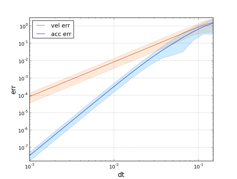
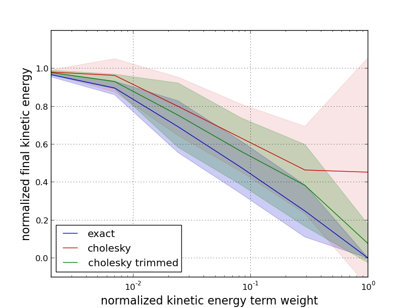
Figure 1: Left: Log-log plot showing convergence of full Hessians to Gauss-Newton Hessians for squared end-effector velocity and acceleration norm terms. As predicted by Theorem 1, the acceleration Hessian shows a faster rate of convergence than the velocity Hessian as indicated by the relative slopes of the linear log-log relations. The plot shows 1 standard-deviation error bars for each progression. Right: Plot showing the efficacy of exact kinetic energy optimization using the Rigid Body Inertial Map derived in Section 4, as well as the Cholesky approximation presented in Section 5 (increasing the energy weight decreases the final energy). The Cholesky approximation usually performs well, but occasionally has difficulty. The trimmed Cholesky progression shows the behavior with outliers removed (see the text for details). Both axes are normalized to lie between 0 and 1; the maximum energy is chosen as the final trajectory energy resulting from optimizing without the energy term, and the minimum energy is the energy resulting from optimizing under the exact kinetic energy using the largest term weight. The plot shows 1 standard-deviation error bars for each progression.

Our first experiment directly addresses convergence and convergence rate of the full Hessian to the Gauss-Newton Hessian as $\Delta t\rightarrow 0$. We defined a smooth nonlinear $8$-dimensional configuration trajectory using the formula

$$q^{(i)}(t)=\frac{\pi}{2}\sin\left(2\pi\sigma_{i}(t-{\scriptstyle\frac{1}{2}})+\eta_{i}\right).$$ (32)

for each joint $i$ (ordered by distance from the base), where $\sigma_{i}\in\mathbb{R}$ ranges linearly from $.5$ to $2$ and $\eta_{i}\in\mathbb{R}$ ranges linearly from $0$ to $\pi$. Time is in units of seconds.

This experiments analyzes the true Hessian of terms of the form

$$\mathcal{F}(\xi)=\sum_{t=1}^{T}\frac{1}{2}\|{\bm{x}}^{(k)}_{t}\|^{2}dt,$$ (33)

where ${\bm{x}}=\phi_{\textrm{fk}}({\bm{q}})$ is the forward kinematics map and $k$ denotes the $k^{\textrm{th}}$-order time derivative. For these experiments, we chose $k=1,2$ to examine task space velocities and accelerations.

Figure 1 shows the basic convergence of the $8\times 8$ diagonal blocks of the true Hessian (calculated using finite-differencing) to the Gauss-Newton Hessian. The plots show the normalized error

$$\textrm{err}({\bm{q}}_{t})=\frac{\|{\bm{H}}_{t}-\widetilde{{\bm{H}}}_{t}\|}{\|{\bm{H}}_{t}\|},$$ (34)

where ${\bm{H}}_{t}$ is the true Hessian block and $\widetilde{{\bm{H}}}_{t}$ is the corresponding Gauss-Newton Hessian block, both scaled by $\Delta t^{2k}$ as suggested by the theory. Here $\|\cdot\|$ denotes the Frobenius matrix norm. We additionally verified separately that the scaled full Hessian and Gauss-Newton Hessian both converge individually to (the same) finite non-zero quantities as $\Delta\rightarrow 0$.

We evaluated the distribution of normalized Hessian block errors across the entire trajectory ($20$ linearly spaced choices of $t$ between $0$ and $1$) for each of the $20$ log-linearly spaced values of $\Delta t$ between $.15$ and $.001$. The plots show the mean and one standard deviation error bars of the normalized errors as a function of $\Delta t$ (in units of seconds). Monomials appear linear in log-log scales; the linearity of these plots verifies the basic form of the predicted convergence rates ($O(\Delta t^{2})$ for the velocity terms and $O(\Delta t^{4})$ for the acceleration terms). Moreover, the slope of the acceleration curve is twice that of the velocity curve verifying the differing relative rates of convergence as well.

6.2 Controlled kinetic energy and Cholesky approximation experiment

We implemented the inertial map derived in Section 4 using a slightly simplified model of the mass distribution. We treat the upper arm and forearm as cylindrical uniformly distributed rigid bodies of mass $9\>\textrm{kg}$ each and use formulas for cylindrical rotational inertia around the appropriate axes to calculate the requisite diagonal components of ${\bm{B}}$ as $b_{1}=.1875\>\textrm{kg\>m}^{2}$, and $b_{2}=b_{3}=.0324\>\textrm{kg\>m}^{2}$ along the principle axes. We model the inertial profile of the hand to be the same as the upper and lower arms but with only $.9\>\textrm{kg}$ of mass.

For this experiment, each of $12$ trials started Apollo (simulated) in one of a collection of initial configurations, and optimized a reach motion to touch one of a collection of points in the 3D space under kinetic energy penalization terms of varying strengths. We used both the exact kinetic energy terms as given by the task space velocity under the Rigid Body Inertial Map described in Section 4 and a Cholesky approximation of the corresponding configuration space kinetic energy formulation using the method described in Section 5. This problem is intentionally simple to provide a more controlled experimental environment for understanding the behavior of the kinetic energy term and it’s Cholesky approximation. In addition to these energy terms, this model used small squared norm terms on configuration space accelerations, initial velocities, and terminal velocities, as well a postural term pulling back to a default configuration for Null space resolution.

The experiments used 6 separate weights for the kinetic energy term log-linearly spaced between 1 and 500, in addition to a weight of 0 (removing the term entirely). The plot shows these weights along the x-axis normalized between 0 and 1. For all nonzero weights, the exact energy term provided an accurate Gauss-Newton Hessian estimate of the problem curvature, and, therefore, optimized very well. We take its final cumulative kinetic energy under the maximal weight as the minimum energy and the final kinetic energy achieved with a weight of 0 as the maximum energy—the reported energy values are scaled linearly between these minimum and maximum values to make them comparable across all scenarios. Figure 1 plots the distribution of achieved normalized energy values as a function of term weight (energy decreases with increased energy penalty term weight).

Generally, the Cholesky approximation performed well. For these trials, though, we intentionally chose the start configuration and reaching target combinations to stress the optimizer. As a result, we found that the Cholesky approximation had difficulty on $4$ of the $12$ trials especially as the term weight became larger as can be seen in the figure. We, therefore, additionally plot the performance of the distribution of the successful $8$ trials as “cholesky trimmed” to show more generally the suboptimality of the approximation when successful.

Understanding better when this Cholesky approximation is good is a subject of future work. When it performs well, it converges very fast, in just slightly more iterations (one or two) than the exact terms under Gauss-Newton Hessians. Our empirical experience, though, emphasizes that, when explicit task maps can be found, they are both fast and highly robust to problem variations.

6.3 Experimental validation on a real-world system

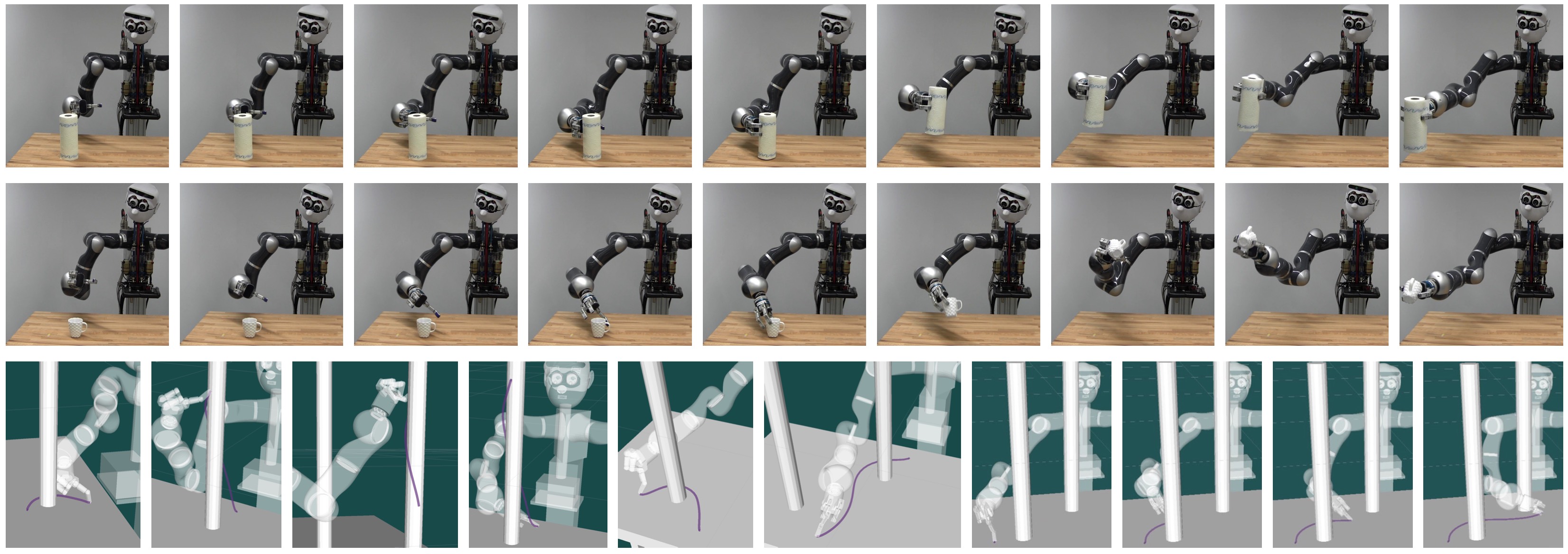
Figure 2: Row 1: Optimizing simultaneous reaching and cylindrical grasp preshaping, and a secondary lift motion with orientational constraints. Row 2: Optimizing reach and elliptical preshaping for a more abnormally shaped object. Row 3: Optimizing motions around thin cylindrical objects using Gauss-Newton Hessians on geometric task maps mapping the workspace to a 9-dimensional latent Euclidean space modeling workspace geometry. The first 6 images show the final configuration of the trajectory and the end-effector trail traced out by the motion; the final 4 images show a sequence of configurations for a single optimized trajectory moving among both cylinders.

Our final experimental demonstrations are on realistic problems using a full implementation of the optimization system for optimized grasp reach and preshaping and obstacle aware motions. Figure 2 shows some of the resulting sequences. Each optimization used $T=30$ and $\Delta t=.1$ seconds.

Our motion model included the following objective terms and constraints:

• Configuration space derivatives penalties. $f({\dot{{\bm{q}}}},{\ddot{{\bm{q}}}})=\alpha_{1}\|{\dot{{\bm{q}}}}\|^{2}+\alpha_{2}\|{\ddot{{\bm{q}}}}\|^{2}$.

• Task space velocity penalties. $f({\bm{x}},\dot{{\bm{x}}})=\frac{1}{2}\|\frac{d}{dt}\phi({\bm{x}})\|^{2}$, where $\phi:\mathbb{R}^{3}\rightarrow\mathbb{R}^{n}$ is a mapping to a workspace geometric space (see [9]). For the grasp preshape experiments, this geometric map was just the identity map.

• Joint limit proximity penalties. $f_{i}(q_{i})=\left(\max\{0,q_{i}-(q_{\mathrm{max}}-\epsilon),(q_{\mathrm{min}}+\epsilon)-q_{i}\}\right)^{2}$, where $\epsilon>0$ is a joint limit margin.

• Posture potentials. $f({\bm{q}})=\frac{1}{2}\|{\bm{q}}-{\bm{q}}_{\mathrm{default}}\|^{2}$ pulling toward a neutral default configuration ${\bm{q}}_{\mathrm{default}}$.

• Kinetic energy. These experiments use a simplified precursor to the more complete kinetic energy model defined in Section 4. The robot was modeled as a collection of point masses at key locations along the robot’s body.

• Joint limit constraints. We have explicit constraints on the joint limits that prevent them from being violated in the final solution.

• Obstacle constraints. All objects are modeled as analytical inequality constraints with a margin. The end-effector, first knuckle, and second knuckle use margins of $0$cm, $1$cm, and $6$cm, respectively; the lower and upper wrist joints use margins of $14$cm and $17$cm, respectively.

• Goal constraint. Reaching the goal is enforced as a zero distance constraint on the goal proximity function. This strategy generalizes the goal set ideas of [1].

The optimizations to grasp preshape configurations used the weighted average position of the fingertips and palm as the end-effector and chose the goal as a point near the centroid of the object. A constraint surface surrounding the object and reflecting the object’s general shape enforced that the fingertip positioning conform to a preshape configuration around the object upon achieving the goal. The cylindrical object used a cylindrical preshape surface in conjunction with final configuration orientation constraint to align the hand to the principle axis of the cylinder; the cup used a simple elliptical preshape surface without orientation constraints. Explicit quadratic potentials pulling the finger joints toward open and close positions at times $\lfloor.75T\rfloor$ and $T$, respectively, implement the open and close behavior of the hand as it approaches the object. After achieving a successful preshape, the robot simply squeezes using compliant control (implemented approximately here simply as torque limits on the fingers and inverse-dynamics of the full arm) in the manner of a pinch grasp. Once kinematic control over the object has been achieved, the robot executes a lift and extend motion additionally optimized by our motion optimizer. The cylindrical lift and extend motion used explicit orientation constraints at each time step to keep the cylinder upright, while the cup lift and extend motion did not. Both final motions used a uniform upward potential in the workspace to implement the lift. We used Gauss-Newton Hessians wherever possible throughout this implementation.

The top two rows of Figure 2 show examples of the reach-preshape, grasp, and lift-extend motions. Each of these motions were optimized starting from the zero motion trajectory in about .7 seconds. This system focused on the motion generation component and did not use a vision system for object localization. The results suggest that an optimization strategy targeting viable preshapes that conform to the general contours of the object, in conjunction with compliant grasping strategies, may constitute a successful interaction approach for objects in unknown environments. A more extensive empirical analysis of this approach integrating vision is the subject of future work.

The final row of the figure shows obstacle avoidance behaviors optimized using latent Euclidean task maps mapping the workspace to a higher-dimensional space that encodes how environmental obstacles warp the geometry of the workspace (see [9]). Each of these motions took between $.3$ and $1$ seconds of computation, using Gauss-Newton Hessians wherever possible.

APPENDIX

1.1 Exploiting Rigid Body Structure

Here we provide some details on the decomposition leading to Equation 13. First, we note that by the definition of center-of-mass,

$${\bm{x}}_{c} =\frac{1}{M}\int{\bm{x}}({\bm{u}})\rho({\bm{u}})d{\bm{u}}=\frac{1}{M}\int\left({\bm{x}}_{c}+\sum_{i}u_{i}{\bm{e}}_{i}\right)\rho({\bm{u}})d{\bm{u}}$$

$$={\bm{x}}_{c}+\frac{1}{M}\sum_{i}\left(\int u_{i}\rho({\bm{u}})d{\bm{u}}\right){\bm{e}}_{i}.$$

And since the set $\mathcal{B}=\{{\bm{e}}_{i}\}_{i=1}^{3}$ forms an orthonormal basis, it must be that

$$\int u_{i}\rho({\bm{u}})d{\bm{u}}=0\ \ \ \textrm{for all}\ \ i=1,2,3.$$ (35)

Now, expanding the kinetic energy expression, we get

$$\frac{1}{2}\int\rho({\bm{u}})\>\|\dot{{\bm{x}}}\|^{2}d{\bm{u}}=\frac{1}{2}\int\rho({\bm{u}})\>\|\dot{{\bm{x}}}_{c}+\sum_{i}u_{i}\dot{{\bm{e}}}_{i}\|^{2}d{\bm{u}}$$

$$\ \ =\frac{1}{2}\int\rho({\bm{u}})\left(\|\dot{{\bm{x}}}_{c}\|^{2}+2\sum_{i}u_{i}\dot{{\bm{x}}}_{c}^{T}\dot{{\bm{e}}}_{i}+\|\sum_{i}u_{i}\dot{{\bm{e}}}_{i}\|^{2}\right)$$

$$\ \ =\frac{1}{2}M\|\dot{{\bm{x}}}_{c}\|^{2}+\sum_{i}\dot{{\bm{x}}}_{c}^{T}\dot{{\bm{e}}}_{i}\int u_{i}\rho({\bm{u}})\>d{\bm{u}}$$

$$\ \ \ \ \ \ \ \ \ \ \ \ \ \ \ \ \ \ \ \ \ \ \ \ \ \ +\frac{1}{2}\sum_{ij}\left(\int u_{i}u_{j}\>\rho({\bm{u}})d{\bm{u}}\right)\dot{{\bm{e}}}_{i}^{T}\dot{{\bm{e}}}_{j}$$

The second term vanishes because of Equation 35, and the first and last terms, together, constitute Equation 13.

1.2 Relationship between the Distributional Inertia Matrix and the traditional Inertia Matrix

It’s fairly straightforward to show, simply from the definition of the traditional inertial matrix ${\bm{I}}$ [12], that the entries of the Distributional Inertia Matrix defined in Section 4 are given by

$${\bm{B}}=\left[{\tiny\begin{array}[]{ccc}\frac{1}{2}(I_{22}+I_{33}-I_{11})&-I_{12}&-I_{13}\\ -I_{21}&\frac{1}{2}(I_{11}+I_{33}-I_{22})&-I_{23}\\ -I_{31}&-I_{32}&\frac{1}{2}(I_{11}+I_{22}-I_{33})\end{array}}\right].$$

The off-diagonal entries of ${\bm{B}}$ are just the negatives of the off-diagonal entries of ${\bm{I}}$, so ${\bm{B}}$ is diagonal if and only if ${\bm{I}}$ is diagonal.

References

- [1] Anca Dragan, Nathan Ratliff, and Siddhartha Srinivasa. Manipulation planning with goal sets using constrained trajectory optimization. In 2011 IEEE International Conference on Robotics and Automation, May 2011.
- [2] Tom Erez, Kendall Lowrey, Yuval Tassa, Vikash Kumar, Svetoslav Kolev, and Emanuel Todorov. An integrated system for real-time model-predictive control of humanoid robots. In IEEE/RAS International Conference on Humanoid Robots, 2013.
- [3] Gianluca Garofalo, Christian Ott, and Alin Albu-Schäffer. On the closed form computation of the dynamic matrices and their differentiations. In IEEE/RSJ International Conference on Intelligent Robots and Systems (IROS), November 2013.
- [4] M. Kalakrishnan, S. Chitta, E. Theodorou, P. Pastor, and S. Schaal. STOMP: Stochastic trajectory optimization for motion planning. In Robotics and Automation (ICRA), 2011 IEEE International Conference on, 2011.
- [5] John M. Lee. Introduction to Smooth Manifolds. Springer, 2nd edition, 2002.
- [6] John Nash. The imbedding problem for Riemannian manifolds. Ann. Math., 63:20–63, 1956.
- [7] Jorge Nocedal and Stephen Wright. Numerical Optimization. Springer, 2006.
- [8] Nathan Ratliff, Marc Toussaint, and Stefan Schaal. Riemannian motion optimization. Technical report, Max Planck Institute for Intelligent Systems, 2015.
- [9] Nathan Ratliff, Marc Toussaint, and Stefan Schaal. Understanding the geometry of workspace obstacles in motion optimization. In IEEE International Conference on Robotics and Automation, 2015.
- [10] Nathan Ratliff, Matthew Zucker, J. Andrew (Drew) Bagnell, and Siddhartha Srinivasa. CHOMP: Gradient optimization techniques for efficient motion planning. In IEEE International Conference on Robotics and Automation (ICRA), May 2009.
- [11] John D. Schulman, Jonathan Ho, Alex Lee, Ibrahim Awwal, Henry Bradlow, and Pieter Abbeel. Finding locally optimal, collision-free trajectories with sequential convex optimization. In In the proceedings of Robotics: Science and Systems (RSS), 2013.
- [12] Bruno Siciliano, Lorenzo Sciavicco, Luigi Villani, and Giuseppe Oriolo. Robotics: Modelling, Planning and Control. Springer, second edition, 2010.
- [13] E. Todorov and W. Li. A generalized iterative lqg method for locally-optimal feedback control of constrained nonlinear stochastic systems. In In proceedings of the American Control Conference, volume 1, pages 300–306, 2005.
- [14] Marc Toussaint. Robot trajectory optimization using approximate inference. In (ICML 2009), pages 1049–1056. ACM, 2009.
- [15] Marc Toussaint. Newton methods for k-order Markov constrained motion problems. CoRR, abs/1407.0414, 2014.