080006 2016 K. Hallberg 080006

The Density Matrix Renormalization Group (DMRG) is a state-of-the-art numerical technique for a one dimensional quantum many-body system; but calculating accurate results for a system with Periodic Boundary Condition (PBC) from the conventional DMRG has been a challenging job from the inception of DMRG. The recent development of the Matrix Product State (MPS) algorithm gives a new approach to find accurate results for the one dimensional PBC system. The most efficient implementation of the MPS algorithm can scale as O($p\times m^{3}$), where $p$ can vary from 4 to $m^{2}$. In this paper, we propose a new DMRG algorithm, which is very similar to the conventional DMRG and gives comparable accuracy to that of MPS. The computation effort of the new algorithm goes as O($m^{3}$) and the conventional DMRG code can be easily modified for the new algorithm.

An efficient density matrix renormalization group algorithm for chains with periodic boundary condition

99 inst1 S. N. Bose National Centre for Basic Sciences, Block JD, Sector III, Salt Lake, Kolkata 700106, India.

1 Introduction

The quantum many-body effect in the condensed matter gives rise to many exotic states such as superconductivity [1], multipolar phases [2, 3], valence bond state [4], vector chiral phase [2, 5] and topological superconductivity [6]. These effects are prominent in the one dimensional (1D) electronic systems due to the confinement of electrons. The confinement of electrons and the competition between the electron-electron repulsion and the kinetic energies of electrons produce many interesting phases like Spin Density Wave (SDW), dimer or the bond order wave phase and Charge Density Wave (CDW) phase in one dimensional systems [7, 8, 9]. Although these quantum many-body effects in the system are crucial for exotic phases, dealing with these systems is a challenging job because of the large degrees of freedom. The degrees of freedom increase as $2^{N}$ or $4^{N}$ for a spin-1/2 system or a fermionic system, respectively.

In most cases, the exact solutions for these systems with large degrees of freedom are almost impossible to reach. Therefore, during the last three decades many numerical techniques have been developed, e.g., Quantum Monte Carlo (QMC) [10], Density Functional Theory (DFT) [11], Renormalization Group (RG) [12] and Density Matrix Renormalization Group (DMRG) method [13, 14]. The DMRG is a state-of-the-art numerical technique for 1D systems with Open Boundary Condition (OBC). However, the numerical effort to maintain the accuracy for PBC systems becomes exponential [15, 16]. It is well known that the Periodic Boundary Condition (PBC) is essential to get rid of the boundary effect of a finite open chain and also to preserve the inversion symmetry in the systems [17].

The DMRG technique is based on the systematic truncation of irrelevant degrees of freedom and has been reviewed extensively in Ref. [15, 16]. In a 1D system with OBC, the number of relevant degrees of freedom is small [15, 16]. Let us consider that for a given accuracy of the OBC system, $m_{\rm{}_{obc}}$ number of eigenvectors of the density matrix is required, then the conventional DMRG for the PBC system requires O($m^{2}_{\rm{obc}}$) [18]. In the conventional DMRG, computational effort for the OBC systems with sparse matrices goes as O($m^{3}_{\rm{obc}}$), whereas, it goes as O($m^{6}_{\rm{obc}}$) for the PBC system [19]. The accuracy of energies for the PBC systems calculated from the conventional DMRG decreases significantly, and there is a long bond in the system which connects both ends.

The accuracy of operators decreases with the number of renormalization, especially the raising/creation $S^{+}/a+$ and lowering/annihilation $S^{-}/a^{-}$ operator of spin/fermionic systems. The conventional DMRG is solved in a $S^{z}$ basis, therefore the exact $S^{z}$ operator remains diagonal and, multiple times, renormalization deteriorates the accuracy slowly; but $S^{+}/a+$ and $S^{-}/a^{-}$ are off diagonal in this exact basis and therefore, the multiple time renormalization of these operators decreases the accuracy of the operators. A similar type of accuracy problems occurs for multiple time renormalized $a^{+}$ and $a^{-}$ in the fermionic systems. In fact, it has been noted that accuracy of energy of a system with PBC significantly increases if the superblock is constructed with very few times renormalized operators [9]. To avoid multiple renormalization, new sites are added at both ends of the chain in such a way that only second time renormalized operators are used to construct the superblock. In this algorithm, there is a connectivity between the old-old sites and their operators are renormalized; and this connectivity spoils the sparsity of the superblock Hamiltonian [9].

In this paper, a new DMRG algorithm is proposed, which can be implemented upon the existing conventional DMRG code in a few hours and gives accurate results which are comparable to those of MPS algorithm. In fact, this algorithm can be implemented for two-legged ladders without much effort [20]. We have studied the spectrum of density matrix of the system block, ground state energy and correlation functions of a Heisenberg anti-ferromagnetic Hamiltonian for spin-1/2 and spin-1 on a 1D chain with PBC.

This paper is divided into five sections. The model Hamiltonian is discussed in section II. The new algorithm and the comparative studies of algorithms are done in section III. The accuracy of various quantities is studied in the section IV. In section V, results and algorithm are discussed.

2 Model Hamiltonian

Let us consider a strongly correlated electronic system where Coulomb repulsion is dominant, therefore the charge degree of freedom gets localized, for example, Hubbard model in large $U$ limit in a half filled band. In this limit, the system becomes insulating, but the electrons can still exchange their spin. The Heisenberg model is one of the most celebrated models in this limit, and only the spin degrees of freedom are active in the model. The Heisenberg model Hamiltonian can be written as

$$H=\sum_{\langle ij\rangle}J_{ij}\vec{S}_{i}\cdot\vec{S}_{j}$$ (1)

where, $J_{ij}$ is the anti-ferromagnetic exchange interaction between the nearest neighbor spin. In the rest of the paper, $J_{ij}$ is set to be 1.

3 Comparison of algorithms

A ground state wavefunction calculated from the conventional DMRG can be represented in terms of the Matrix Product State (MPS), as shown by Ostlund and Rommer [21]. The wavefunction can be written as

$$|\psi\rangle=\sum_{n_{1},n_{2},\ldots,n_{L}}{\rm{tr}}(A_{n_{1}}^{1}A_{n_{2}}^{2}\ldots A_{n_{L}}^{L})|n_{1},n_{2},\ldots,n_{L}\rangle,$$ (2)

where $A_{n_{k}}^{k}$ are a set of matrices of dimension $m\times m$ for site $k$ and with $n_{k}$ degrees of freedom. The wave function $|\psi\rangle$ can be accurately found if $m$ is sufficiently large. The expectation value of an operator $O_{k}$ in the gs [19, 22] can be written as

$$\langle O_{k}\rangle={\rm{tr}}\left(\sum_{n_{k},n^{{}^{\prime}}_{k}}\langle n_{k}|O_{k}|n^{{}^{\prime}}_{k}\rangle A_{n_{k}}^{k}\otimes A_{n^{{}^{\prime}}_{k}}^{k}\right),$$ (3)

where $n_{k}$ is the local degrees of freedom of site $k$. The matrix $A$ can be evaluated by using the following equations

$$H_{k}|\psi_{k}\rangle =\lambda N_{k}|\psi_{k}\rangle,$$ (4)

$$N^{k} =E_{1}^{k+1}E_{1}^{k}\ldots E_{1}^{L}E_{1}^{1}\ldots E_{1}^{k-1},$$ (5)

where

$$E_{1}^{k}=\sum_{n_{k},n^{{}^{\prime}}_{k}}\langle n_{k}|1|n^{{}^{\prime}}_{k}\rangle A_{n_{k}}^{k}\otimes A_{n^{{}^{\prime}}_{k}}^{k}.$$ (6)

Here, $H_{k}$ is the effective Hamiltonian of $k^{\rm{th}}$ site and $\lambda$ is the expectation value of energy. The $A$ matrices are evaluated at this point and the matrices are rearranged to keep the algorithm stable. The $H_{k}$ and $N$ can be calculated recursively while evaluating $A$, one site at a time [19]. Here, $N$ matrices are ill-conditioned and require storing, approximately $L^{2}$ matrices as well as multiplication of $L^{2}$ matrices of $m\times m$ size [19] at each step. The evaluation of $A$ and $N$ are done for all the sites and backward and forward sweeps for all the sites are executed similarly to the finite system DMRG. The mathematical operations of matrices of dimension $m^{2}\times m^{2}$ represent the Hamiltonian cost $\sim(o)m^{6}$, but the special form of these matrices reduces the cost by a factor of $m$. Therefore, this algorithm scales as $\sim(o)m^{5}$ [19].

The above algorithm is extended by Verstraete et. al., for translational invariant systems [23]. Only two types of matrices, $A^{1}$ and $A^{2}$, are considered [23]. Product of the two matrices can be repeated to compute $N$. In this algorithm, only two matrices, $A^{1}$ and $A^{2}$, are updated and optimized to get the gs properties. This algorithm scales as (o)$m^{3}$, although it does not work for a finite system, or systems with impurity, etc. Pippan et. al. introduced another MPS based efficient algorithm for translational invariant PBC systems [19]. In the old version of MPS, most of the computation cost goes to constructing the product of $m^{2}\times m^{2}$ matrices $E$ defined in Eq. (6). The new MPS algorithm overcomes this problem by performing a SVD of the product of sufficiently large $(l\gg 1)$ number of $m^{2}\times m^{2}$ transfer matrices[19, 28]. The singular values, in general, decay very fast; therefore, only $p\,(\ll m^{2})$ among $m^{2}$ singular values are significant [28]. Thus, the computational cost now is reduced to (o) $p\times m^{3}$ [19]. However, one requires $p\sim m$ to reach adequate numerical accuracy of physical measures, as pointed out in Ref. [28].

Although the above technique is efficient and accurate, there are various reasons for developing the new algorithm. First, the modified MPS works efficiently for a system where the singular values of products of matrices decay exponentially and this algorithm scales as (o) $pm^{3}$, where $p$ can vary linearly with $m$. Second, the implementation of the MPS based numerical technique is quite different from the conventional DMRG, and the MPS algorithm should be written from scratch. Third, many conventional numerical techniques like the dynamical correction vector [24] or continued fraction [25], and implementation of symmetries like parity or inversion symmetries are difficult. In this paper, we will explain a new algorithm which is very similar to the conventional DMRG technique, and also show that the new algorithm can give accuracy comparable to that of MPS based techniques. This algorithm is applied for $S=1/2$ and $S=1$ chains with PBC. But first, let us try to understand the algorithm before discussing the results.

In this algorithm, we will try to avoid the multiple renormalization of operators, whereas the other parts of the algorithm remain the same as the conventional DMRG. Before going to the new algorithm, let us recap the conventional DMRG.

1. Start with a superblock of four sites consisting of one site for both the left and the right block and two new sites.

2. Get desired eigenvalues and eigenvectors of the superblock and construct the density matrix $\rho$ of the system which consists of the left or the right block and a new site.

3. Now, construct an effective $\tilde{\rho}$ with $m$ number of eigenvectors of $\rho$, corresponding to the $m$ largest eigenvalues. The effective system Hamiltonian and all operators in the truncated basis are constructed using the following equations:

   $$H=\tilde{\rho}^{\dagger}H\tilde{\rho};\qquad O=\tilde{\rho}^{\dagger}H\tilde{\rho}$$ (7)

4. Superblock is constructed using the effective Hamiltonian and operators of the system block and two new sites.

5. Repeat all the steps from 2 until the desired system size is reached. The full process is called infinite DMRG.

As mentioned earlier, the conventional algorithm is excellent for a 1D open chain as superblock is constructed with only one time renormalized operators. However, for a PBC system, one needs a long bond; therefore, at least two operators of superblocks are renormalized multiple times. In the new algorithm, the multiple time renormalization of operator is avoided and the algorithm goes as:

1. Start with a superblock with four blocks consisting of a left and a right block and two new site blocks. The blocks are shown in Fig. 1 as filled circles and may have more than one site. Here, we have considered only one site in each block. New blocks may also have more than one site and are shown as open circles. In this paper, new blocks have one site in a chain or two for a ladder, like a structure with PBC [17].

   

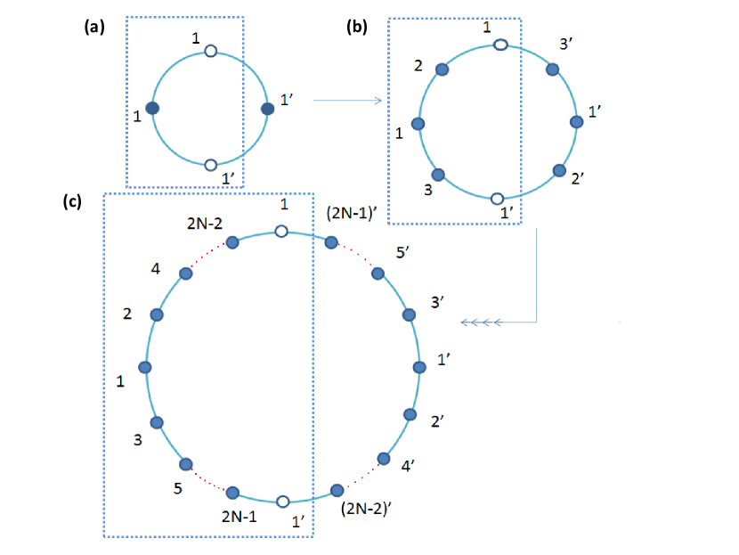
   Figure 1: Pictorial representation of the new DMRG algorithm with only one site in the new block. (a) One starts with two blocks left and right represented by filled circles and two new sites blocks represented as open circles. The dotted box represents the system block for the next step. (b) Superblock of the next DMRG step is shown. (c) The final step of infinite DMRG of $N=4N$ system size is shown with $2N-1$ number of sites in each of the left and the right blocks and two new sites.

2. Get the eigenvalues and eigenvectors of the superblock and construct the density matrix $\rho$ of the system which consists of the left or the right block and two new blocks. The left system block is shown inside the box in Fig. 1a.

3. Now, construct an effective $\tilde{\rho}$ with $m$ number of eigenvectors of $\rho$ corresponding to the $m$ largest eigenvalues of the density matrix. The effective system Hamiltonian and operators in the truncated basis are calculated using Eq. (7).

4. The superblock is constructed using the effective Hamiltonian and operators of system blocks and two new sites.

5. Now, go to step 2 and the processes 2 – 5 are repeated till the desired system size is reached.

We notice that the superblock Hamiltonian is constructed using the effective Hamiltonian of blocks and operator which are renormalized once. Therefore, the massive truncation because of long bond is avoided in this algorithm. Bonds in the superblock are only between new-new sites or new-old sites. For the construction of a Hamiltonian matrix of old-new site bond, a new site operator is highly sparse. However, old sites renormalized operators are highly dense. The old-old sites interaction in the conventional algorithm generates a large number of non-zero matrix elements in the superblock Hamiltonian matrix and the diagonalization of dense matrix goes as $m^{4}$. But, in the new algorithm, old-new sites interaction in the superblock generates only a sparse Hamiltonian matrix, and its digonalization scales as $m^{3}$.

4 Results

We consider spin-1/2 and spin-1 chains with PBC of length up to $N=500$ to check the accuracy of results for the Heisenberg Hamiltonian. In this part, we study the truncation error of density matrix $T$, error in relative ground state energy $\frac{\Delta E}{|E_{0}|}$ and dependence of correlation function $C(r)$ on $m$. The correlation function $C(r)$ is defined as

$$C(r)=\vec{S}_{0}\cdot\vec{S}_{r},$$ (8)

where $\vec{S}_{0}$ corresponds to the reference spin and $\vec{S}_{r}$ is the spin at a distance $r$ from the reference spin. The relative ground state energy can be defined as $\Delta E/|E_{0}|$, where $\Delta E=E(m)-E_{0}$ with $E_{0}$ is the most accurate value for $S=1$ chain [19] and $E_{0}=E(m=1200)$ for $S=1/2$ chain.

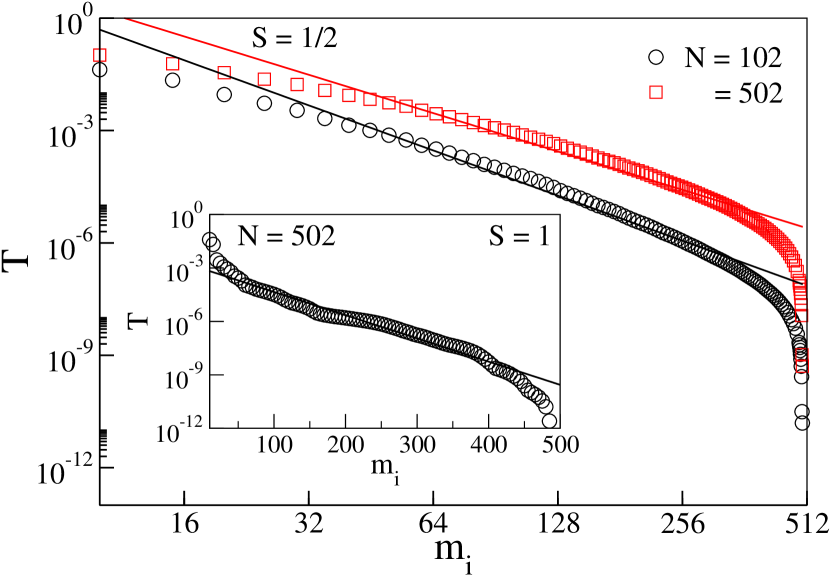
Figure 2: Truncation error $T$ of the density matrix for spin-1/2 chain (main). The inset shows the truncation error for the $S=1$ chain. For $S=1/2$, the truncation error follows power law decay whereas it follows exponential decay for a $S=1$ system.

As discussed earlier, the DMRG is based on the systematic truncation of the irrelevant degrees of freedom and the eigenvalues of the density matrix represent the importance of the respective states. In the DMRG, only selected states corresponding to the highest eigenvalues are kept and the rest of the other states are thrown. We define truncation error $T$ as

$$T=1-\sum_{i=1}^{m}\lambda_{i}$$ (9)

where $\lambda_{i}$ are eigenvalues of density matrix of the system block arranged in descending order. In the main Fig. 2, $T$ is shown as function of $m$ for $S=1/2$ and the inset shows the same for a $S=1$ system with N=102 and 502. We notice that $m\sim 350$ for $S=1/2$ and $m\sim 300$ for $S=1$ are sufficient to achieve $T=10^{-9}$. In the main Fig. 2, $T$ vs $m$ in a log-log plot shows a linear behavior, i.e., $T$ for both system sizes of $N=102$ and 502 for $S=1/2$ follows a power law $T\propto m_{i}^{\alpha}$ with $\alpha=4.0$ and 3.4, respectively. The $m$ dependence of $T$ for $S=1$ ring is shown in the inset of Fig. 2. The truncation error $T$ in this case decays exponentially, i.e., $T\propto\exp(-\beta m_{i})$ with $\beta=0.03$ for both $N=102$ and 502.

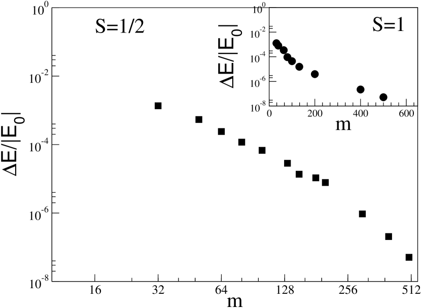
Figure 3: Energy accuracy $\Delta E/|E_{0}|$ for spin half chain with PBC (main) which shows a power law behavior with $m$. The inset shows the energy accuracy for spin one chain with PBC which shows exponential behavior with $m$.

The relative error in energies $\Delta E/|E_{0}|$ for $S=1/2$ and 1 with $N=102$ spins are shown in Fig. 3, main and inset respectively. The exact energies of a spin-1 system is $E_{0}/N\sim−1.4014840386$ and this value is obtained by using conventional DMRG with $m=2000$ and up to $N=100$ site chain [19]. Extrapolation of energies with $m$ is done to obtain the above value [19]. We notice that $\frac{\Delta E}{E_{0}}$ for $S=1/2$ systems goes to $10^{-6}$ for $m=256$ whereas it goes to $10^{-8}$ for $m\approx 500$, as shown in the main Fig. 3. Although similar accuracy of the energy can be achieved with $m=100$ in MPS approach, the scaling is $\sim m^{4}$, rather than $\sim m^{3}$ in our algorithm. For $S=1$ accuracy of $10^{-8}$ can be reached with $m\sim 450$, as shown in the inset of Fig. 3.

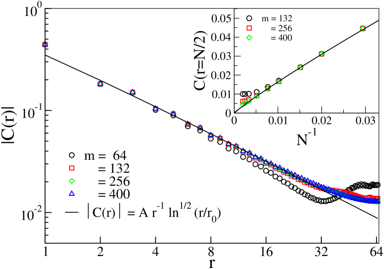
Figure 4: The main figure shows the variation of $|C(r)|$ (defined in Eq. (8)) as a function of $r$ for different $m$. The solid curve in the main figure is the logarithmic correction formula: $Ar^{-1}\ln^{1/2}(r/r_{0})$ with $A=0.22$ and $r_{0}=0.08$. [29, 26] The inset shows the variation of $C(N/2)$ with the inverse of $N$ for different $m$. The solid curve is the form: $A(N/2)^{-1}\ln^{1/2}(N/2r_{0})$ with $A=0.323$ and $r_{0}=0.08$.

The dependence of accuracy of correlation function $|C(r)|$ of $S=1/2$ for $N=130$ as a function of $m$ is shown in the main Fig. 4. We notice that $m=256$ is sufficient to achieve an accuracy of $\sim 10^{-4}$. We also notice that $|C(r)|\propto r^{-1}$ with the well known logarithmic correction specially for smaller $r$ [26]. We have fitted the correlations with the well known form $|C(r)|=Ar^{-1}\ln^{1/2}(r/r_{0})$ with $A=0.22$ and $r_{0}=0.08$ [29]. Deviation in function for large $r$ is the artifact of finite systems. In our algorithm, two sites are added symmetrically and the new sites are added $N/2$ sites apart, consequently the distance between two new sites is $N/2$. Therefore, the new-new sites correlation function is $C(N/2)$ and is plotted with $N^{-1}$ in the inset of Fig 4. We observe that $m=256$ is sufficient for $N\sim 200$ to achieve sufficient numerical accuracy. The curve behaves almost linearly with the logarithmic correction: $|C(N/2)|=2AN^{-1}\ln^{1/2}(N/2r_{0})$ with $A=0.323$ and $r_{0}=0.08$.

5 Summary

The DMRG is a state-of-the-art numerical technique for solving the 1D quantum many-body systems with open boundary condition. However, the accuracy of the 1D PBC system is rather poor. The MPS approach gives very accurate results but the computational cost goes as (o) $m^{5}$ [23]. Later, this algorithm was modified and the computational cost of the modified algorithm goes as (o) $p\times m^{3}$, where $p$ in general varies linearly with $m$ [28], but $p$ can go as $m^{2}$ in case of long range order in the system. The computational cost of the algorithm presented in this paper scales as (O) $m^{3}$ because of the sparse superblock Hamiltonian and is very similar to the conventional DMRG. To achieve this goal, we avoid the multiple times renormalization of the operators which are used to construct the superblock. This algorithm can readily be used to solve general 1D and quasi-1D systems, e.g., $J_{1}$–$J_{2}$ model, two-legged ladder. The new algorithm can be implemented with ease using the conventional DMRG code.

Our calculation suggests that most of the quantities, e.g., ground state energies, energy gaps and correlation function, can accurately be calculated by keeping $m\sim 400$. The superfluity stiffness [27] and dynamical structure factors using the correction vector technique [24] or continued fraction method [25] can be calculated with this algorithm. The symmetries, e.g., spin parity, electron-hole, inversion, can easily be implemented in this algorithm [24]. This algorithm is used by us in calculating accurate static structure factors and correlation function for $J_{1}-J_{2}$ model for a spin-1/2 ring geometry [17].

- [1] M Tinkham, Introduction to Superconductivity: Second Edition (Dover Books on Physics) (Vol I), Dover Publications INC, New York (2004).
- [2] A V Chubukov, Chiral, nematic, and dimer states in quantum spin chains, Phys. Rev. B 44, 4693 (1991).
- [3] L Kecke, T Momoi, A Furusaki, Multimagnon bound states in the frustrated ferromagnetic one-dimensional chain, Phys. Rev. B 76, 060407 (2007).
- [4] P W Anderson, The resonating valence bond state in la2cuo4 and superconductivity, Science 235, 1196 (1987).
- [5] A Parvej, M Kumar, Degeneracies and exotic phases in an isotropic frustrated spin-1/2 chain, J. Magn. Magn. Mater. 401, 96 (2016).
- [6] X L Qi, S C Zhang, Topological insulators and superconductors, Rev. Mod. Phys. 83, 1057 (2011).
- [7] M Nakamura, Tricritical behavior in the extended hubbard chains, Phys. Rev. B 61, 16377 (2000).
- [8] P Sengupta, A W Sandvik, D K Campbell, Bond-order-wave phase and quantum phase transitions in the one-dimensional extended hubbard model, Phys. Rev. B 65, 155113 (2002).
- [9] M Kumar, S Ramasesha, Z G Soos, Tuning the bond-order wave phase in the half-filled extended hubbard model, Phys. Rev. B 79, 035102 (2009).
- [10] M Suzuki (Ed.), Quantum Monte Carlo Methods in Condensed Matter Physics, World Scientific, Singapore (1993).
- [11] W Kohn, L J Sham, Self-consistent equations including exchange and correlation effects, Phys. Rev. 140, A1133 (1965).
- [12] K G Wilson, The renormalization group and critical phenomena, Rev. Mod. Phys. 55, 583 (1983).
- [13] S R White, Density matrix formulation for quantum renormalization groups, Phys. Rev. Lett. 69, 2863 (1992).
- [14] S R White, Density-matrix algorithms for quantum renormalization groups, Phys. Rev. B 48, 10345 (1993).
- [15] U Schollwöck, The density-matrix renormalization group, Rev. Mod. Phys. 77, 259 (2005).
- [16] K A Hallberg, New trends in density matrix renormalization, Adv. Phys. 55, 477 (2006).
- [17] Z G Soos, A Parvej, M Kumar, Numerical study of incommensurate and decoupled phases of spin-1/2 chains with isotropic exchange , between first and second neighbors, J. Phys. Condens. Mat. 28, 175603 (2016).
- [18] U Schollwöck, The density-matrix renormalization group in the age of matrix product states, Ann. Phys. 326, 96 (2011).
- [19] P Pippan, S R White, H G Evertz, Efficient matrix-product state method for periodic boundary conditions, Phys. Rev. B 81, 081103 (2011).
- [20] E Dagotto, T M Rice, Surprises on the way from one- to two-dimensional quantum magnets: The ladder materials, Science 271, 618 (1996).
- [21] S Östlund, S Rommer, Thermodynamic limit of density matrix renormalization, Phys. Rev. Lett. 75, 3537 (1995).
- [22] F Verstraete, D Porras, J I Cirac, Density matrix renormalization group and periodic boundary conditions: A quantum information perspective, Phys. Rev. Lett. 93, 227205 (2004).
- [23] F Verstraete, J I Cirac, J I Latorre, E Rico, M M Wolf, Renormalization-group transformations on quantum states, Phys. Rev. Lett. 94, 140601 (2005).
- [24] S K Pati, S Ramasesha, Z Shuai, J L Brédas, Dynamical nonlinear optical coefficients from the symmetrized density-matrix renormalization-group method, Phys. Rev. B 59, 14827 (1999).
- [25] K A Hallberg, Density-matrix algorithm for the calculation of dynamical properties of low-dimensional systems, Phys. Rev. B 52, R9827 (1995).
- [26] I Affleck, D Gepner, H J Schulz, T Ziman, Critical behaviour of spin-s Heisenberg antiferromagnetic chains: analytic and numerical results, J. Phys. A - Math. Gen. 22, 511 (1989).
- [27] D Rossini, V Giovannetti, R Fazio, Spin-supersolid phase in Heisenberg chains: A characterization via matrix product states with periodic boundary conditions, Phys. Rev. B 83, 140411 (2011).
- [28] D Rossini, V Giovannetti, R Fazio, Stiffness in 1D matrix product states with periodic boundary conditions, J. Stat. Mech. 2011, P05021 (2011).
- [29] A W Sandvik, Computational Studies of Quantum Spin Systems, AIP Conf. Proc. 1297, 135 (2010).