Pattern formation with repulsive soft-core interactions: discrete particle dynamics and Dean-Kawasaki equation

Abstract

Brownian particles interacting via repulsive soft-core potentials can spontaneously aggregate, despite repelling each other, and form periodic crystals of particle clusters. We study this phenomenon in low-dimensional situations (one and two dimensions) at two levels of description: performing numerical simulations of the discrete particle dynamics, and by linear and nonlinear analysis of the corresponding Dean-Kawasaki equation for the macroscopic particle density. Restricting to low dimensions and neglecting fluctuation effects we gain analytical insight into the mechanisms of the instability leading to clustering which turn out to be the interplay between diffusion, the intracluster forces and the forces between neighboring clusters. We show that the deterministic part of the Dean-Kawasaki equation provides a good description of the particle dynamics, including width and shape of the clusters, in a wide range of parameters, and analyze with weakly nonlinear techniques the nature of the pattern-forming bifurcation in one and two dimensions. Finally, we briefly discuss the case of attractive forces.

I Introduction

Ensembles of interacting random walkers and their description in terms of densities appear in many contexts ranging from biological or physical to social phenomena Grimm2005 ; Bonabeau2002 ; Topaz2006 ; Chavanis2008a ; Marchetti2013 ; Pineda2010 . Usually these interactions act locally, involving only a few individuals, but they induce global patterns of behavior of the full system like phase transitions, the formation of periodic spatial structures, collective movement and synchronization states. Knowing the conditions for the formation of these collective structures and its own feedback on the dynamics is a central issue in the understanding of complex systems. The study of these individual-based models is approached from two complementary points of views: a) the particle description, describing the dynamics of individuals and their interactions, and based mainly on numerical simulations; and b) the continuum description in terms of evolution equations for the local density (or another macroscopic field).

In physical systems forces drive particle motions, and they are usually derived from two-body potentials acting repulsively or attractively at different distances. This is the case of many forces, like the Lennard-Jones case, among atoms and molecules in liquids, polymer and colloidal solutions. In biological systems facilitation and competition mechanisms at short and large scales also drive organism motion, but they can in addition modulate growth and death rates Murray2004 ; Okubo2001 . The interplay between facilitation and competition at different distances, but specially the effect of competition, has been shown to be responsible for the formation of periodic arrangements of clusters of particles and more complex structures Hernandez2004 ; Hernandez2014 ; Schellinck2011 ; MartinezGarcia2015 , which are related to the appearance of vegetation patterns and periodic aggregations of bacteria Borgogno2009 ; Martinez2014 ; BenJacob2000 ; Ramos2008 ; Rietkerk2008 ; Meron .

There is however a recently discovered situation, relevant to polymer and colloidal solutions, where the same effect is observed for particle systems interacting with soft-core forces which are repulsive at all distances Klein1994 ; Likos2001 ; Mladek2006 ; Likos2007 ; Mladek2008 ; Coslovich2013 : a liquid-solid transition occurs, but in the solid the unit cell is not occupied by one particle or molecule, but by a closely packed cluster of them, forming a so-called cluster crystal. Note the counter-intuitiveness of this phenomenon: despite all particles are repelling, they aggregate. Beyond condensed-matter systems this is a phenomenon analogous to the aggregation of reproducing organisms occurring despite purely competitive interactions Hernandez2004 ; MartinezGarcia2013 ; Hernandez2014 .

This cluster crystallization transition has been analyzed with equilibrium statistical mechanics tools, including Monte-Carlo simulations, in three-dimensional systems Likos2001 ; Mladek2006 ; Likos2007 ; Mladek2008 ; Coslovich2013 . However, approaches exploiting non-linear dynamics and pattern formation techniques Walgraef2012 can add insight to the study of this instability, including dynamic regimes. This was in fact the route followed in the early work by Munakata Munakata1977 , but the lack of numerical simulations there hindered the identification of several relevant features, as for example the dominance of hexagonal patterns instead of stripes in two dimensions. In addition, identification and understanding of relevant mechanisms become much clearer when considering low-dimensional (one- and two-dimensional) systems, as compared with the complexity of three-dimensional structures. The central objective of this paper is to analyze in detail the processes leading to cluster crystals in one-dimensional (1d) and two-dimensional (2d) systems of soft-core repulsive particles providing when possible analytical insight. The physical mechanisms leading to this cluster formation are discussed in detail. Our approach is similar in spirit to the one used in Archer2013 ; Archer2015 , where 2d crystals arising from competing interactions at two spatial scales were considered, but here we restrict to the simpler case of a single interaction scale for which greater and more complete understanding can be achieved. For completeness, we consider briefly also the case of purely attracting interactions, highlighting some similarities and differences between both cases.

The paper is organized as follows: In Section II we start our study with an overdamped Brownian dynamics, which is relevant in freezing, the glass transition, colloidal systems, or bacterial patterns, and investigate the effect of repulsive interactions, leading to cluster crystals, by performing numerical simulations of the particle dynamics. In Sec. III we analyze a deterministic integrodifferential model, the Dean-Kawasaki (DK) equation Kawasaki1994 ; Dean1996 ; Munakata1977 ; Kim2014 , showing that it gives an appropriate description of the particle dynamics and give analytical arguments for the findings of the previous section. In particular we obtain analytical results for the pattern formation transition and for the shape of the pattern and of the clusters forming it. For completeness, we briefly consider attractive interactions in Sect. IV both for the particles and for the DK model. Finally, in Sec. V we give a discussion and summary of the main results.

II Brownian particles with soft-core repulsive interactions

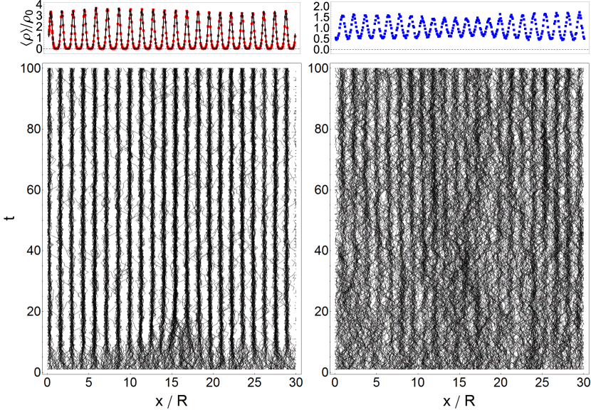
Figure 1: Dynamics of a system of 6000 particles evolving according to Eq. (3) in a periodic one-dimensional domain of size $L=3$, so that $\rho_{0}=2000$. The interaction potential is GEM-3 with parameters $R=0.1$ and $\epsilon=0.0333$. Left, $D=0.4$ so that $\tilde{D}=D/(\epsilon\rho_{0}R)=0.06$. Right: $D=0.6$ so that $\tilde{D}=0.09$. The lower panels show the spatiotemporal trajectories (in black). For clarity of the plots, only $600$ trajectories are shown here. The top panels show a coarse-grained normalized density, $\left<\rho(x)\right>/\rho_{0}$, at the late stages. The coarse-graining is done by averaging spatially over boxes of width $0.02R$ and temporally over the last $150$ temporal configurations separated by $10^{-3}$ time units. In the top left panel, the clusters are fitted by Gaussians (black lines).

In the overdamped limit, the motion of $N$ point particles at positions $\{{\bf x}_{1},{\bf x}_{2},...,{\bf x}_{n}\}$ in $d$-dimensional space, with friction coefficient $\gamma$, subjected to Brownian motion and interacting with a potential energy $U=\gamma V$ is given by

$$\dot{\bf x}_{i}=-\nabla_{i}V({\bf x}_{1},{\bf x}_{2},...,{\bf x}_{n})+\sqrt{2D}~{}{\boldsymbol{\xi}}_{i}(t)\ ,$$ (1)

with independent Gaussian noise vectors ${\boldsymbol{\xi}}_{i}$ satisfying

$$\left<{\boldsymbol{\xi}}_{i}\right>=0\ ,\ \left<{\boldsymbol{\xi}}_{i}(t){\boldsymbol{\xi}}_{j}(t^{\prime})\right>=\mathbb{I}\delta_{ij}\delta(t-t^{\prime})\ .$$ (2)

$\mathbb{I}$ is the $d$-dimensional identity. When noise is of thermal origin the diffusion coefficient $D$ is proportional to temperature according to Einstein’s relation $D=k_{B}T/\gamma$. $\nabla_{i}$ denotes the gradient with respect to the position ${\bf x}_{i}$. The system’s mean density is given by $\rho_{0}=N/L^{d}$ ($L^{d}$ the total $d-$volume) and remains constant since the total number of particles is conserved. In the following we will assume pairwise interactions, so that $V({\bf x}_{1},...{\bf x}_{N})=\frac{1}{2}\sum_{ij}v({\bf x}_{i}-{\bf x}_{j})$, and (1) becomes

$$\dot{\bf x}_{i}=-\sum_{j=1}^{N}\nabla v({\bf x}_{i}-{\bf x}_{j})+\sqrt{2D}~{}{\boldsymbol{\xi}}_{i}(t).$$ (3)

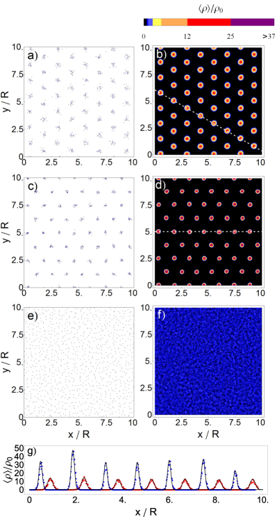
Figure 2: Left column: snapshots of the positions of $N=1000$ particles in 2d at large times for $R=0.1$, $\epsilon=0.0333$, $L=1$ and $\rho_{0}=1000$. Right column: coarse-grained densities of the same configurations. The coarse-graining is done by averaging in space over distances $0.017R$ and in time over $500$ configurations separated by $10^{-3}$ time units. a) and b) GEM-3 potential with $D=0.02$ so that $\tilde{D}=D/(\epsilon\rho_{0}R^{2})=0.06$. c) and d) GEM-3 potential with $D=0.01$ ($\tilde{D}=0.03$). e) and f) GEM-1 potential with $D=0.005$ ($\tilde{D}=0.015$). Figure g) is the density $\rho$ along the white dotted lines shown on Figs. b) and d) (red and blue squares respectively). The black curves correspond to a fit by a sum of Gaussian functions.

Following previous works Mladek2006 ; Likos2007 we consider the generalized exponential model of exponent $\alpha$ (GEM-$\alpha$) as interaction potential:

$$v({\bf x})\equiv\epsilon\exp\left(-\left|\frac{{\bf x}}{R}\right|^{\alpha}\right)\ .$$ (4)

This is a convenient and flexible family of interactions sharing the property of soft-core that will be relevant for the cluster crystallization. By soft-core we mean that the potential does not diverge at ${\bf x}=\bf 0$ so that the particles can overlap. The width $R$ indicates the spatial range of the interaction, and $\epsilon$ its magnitude. $\epsilon$ is positive for the repulsive interactions mostly considered here, and will be taken to be negative in Sect. IV to model attractive interactions. For $\alpha<2$ GEM-$\alpha$ potentials are more peaked at zero, and they get more box-like as $\alpha$ increases. It is known Bochner1937 ; Likos2007 that GEM-$\alpha$ potentials with $\alpha>2$ have both positive and negative Fourier components, while for $\alpha\leq 2$ the Fourier transform is strictly positive. These will be important properties as we will see later. In our simulations two representative kinds of GEM potentials are used: a GEM-1 and a GEM-3 potential, although results for other values of $\alpha$ will be mentioned.

Numerically we observe that for large diffusion coefficients or any GEM-$\alpha$ potential with $\alpha<2$ the particle distribution remains rather unstructured in time. For GEM-$\alpha$ with $\alpha>2$, however, a periodic modulation in the particle distribution arises when decreasing the diffusion coefficient or increasing the density. This is seen in Figure 1, that shows spatiotemporal trajectories of a one-dimensional system of Brownian particles moving according to Eq. (3) with repulsive interaction GEM-3, starting from an initial random distribution. For sufficiently small $D$, particle distribution becomes a periodic array of well separated clusters. This is a cluster crystal as each cluster is made of many particles which remain very close, despite they repel each other. Also in Fig. 1 we show a coarse-graining of the particle distribution at the latest times, showing that the configuration is essentially an array of Gaussian clusters for small $D$, approaching a sinusoidal modulation when increasing $D$ towards the disappearance of the pattern. By slowly incrementing $D$ in our particles simulations, we determined that this occurs at $D_{c}\approx 0.68$ for the parameters used in that figure.

In Figure 2, we plot results from 2d simulations of the particle system under the GEM-3 and the GEM-1 potentials. Left column shows long-time distributions of the particles for these two interacting potentials and for different values of the control parameters, while in the right column we show the coarse-grained density functions. It clearly appears on Fig. a) and c) that hexagonal patterns can spontaneously appear for the GEM-3 potential. The corresponding densities in the right column exhibit peaks that can be fitted by two-dimensional Gaussians as can be seen in Fig.  2 g). The width of the peak $\sigma$ and the distance $a$ between them are functions of the control parameters as we will see later on. For a given GEM-3 potential, these patterns disappear when $D$ is increased, or when either $\rho_{0}$, $R$ or $\epsilon$ are decreased. On the other hand, persistent clusters are never observed for particles interacting with the GEM-1 potential. In those cases, the late time state is always statistically homogeneous as in Fig.  2 e), f).

The structure of the system is conveniently analysed by computing the radial distribution function $g^{(2)}(r)$ and the structure factor $S(q)$ given by

$$g^{(2)}({\bf x}) = g^{(2)}(r)=\frac{1}{\rho_{0}}\langle\sum_{i\neq 0}\delta({\bf x}-{\bf x}_{i})\rangle,$$ (5)

$$S({\bf q}) = S(q)=1+\rho_{0}\int d{\bf x}e^{-i{\bf q}\cdot{\bf x}}\left(g^{(2)}({\bf x})-1\right).$$ (6)

The sum in (5) is over particles different from a reference particle at the origin, and the average is over positions ${\bf x}$ at the same distance $r=|{\bf x}|$ from there. Figure 3 a) shows that the radial distributions of systems with GEM-3 potentials have several peaks. The first one, at $r=0$, corresponds to particles belonging to the same cluster while the second peak tells us the typical distance $a$ between two neighboring clusters. The height of the peaks is proportional to how “ordered” the system is so that it decreases for larger diffusion coefficients. It is also interesting to note that the $r=0$ peak completely disappears for the GEM-1 potential and can thus be considered as a signature of the $\alpha>2$ clustering, in which the ultra-soft potentials allow particles to concentrate at very short distances. The structure factor $S(q)$, which can be calculated from the Fourier transform of $g^{(2)}(r)$, also has a clearly visible peak at the wavelength $q=2\pi/a$. Its amplitude $S_{max}$ decreases when $D$ increases as can be seen in Fig.  3 c) with scaled units. It also decreases for decreasing $R$, $\rho_{0}$ and $\epsilon$. The change of $S_{max}$ with respect to $D$ underlines the transition from periodic patterns to homogeneous equilibrium states as it abruptly jumps down to $S_{max}\approx 1$ for a critical value of $D_{c}$.

It should be noted that, according to Peierls argument Peierls1935quelques , we do not expect a true crystal with long-range order in one-dimension if $D$ (proportional to temperature) is non-zero. Also, although standard theorems on absence of phase transitions do not apply to the soft-core potential used here Cuesta2004 , it seems that true thermodynamic phase transitions do not occur in this type of models in one dimension Prestipino2015 . Thus, when referring to states such as the ones displayed in Fig. 1 as cluster crystals we do not imply the existence of any true thermodynamic solid-liquid phase transition, but simply highlight that the local organization of the particle distribution at small $D$ is very different and more clustered and periodic than the nearly homogeneous state found at large $D$. When neglecting fluctuations, however, the transition becomes a true bifurcation, as will be seen in Sect. III. It will also be shown there that this deterministic approximation gives a reasonable description if not too close to the bifurcation point. The situation in 2d is more subtle, because of the peculiarities of two-dimensional melting Strandburg1988 . We will not address here the nature of the crystal-liquid transition in this soft-core system Gasser2009 ; Zu2016 . We just note that the approximate scaling of $S_{max}$ with $N=\rho_{0}L^{2}$ (Fig. 3c) suggests the presence of some translational order in the system. As in the 1d case, the deterministic approach described in the next section provides useful insight of the mechanisms at work and even quantitative description of the observations in some parameter range.

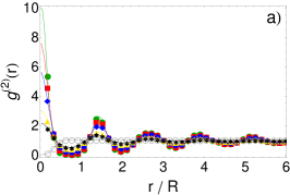
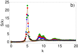
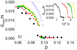
Figure 3: a) Radial distribution function $g^{(2)}(r)$ and b) structure factor $S(k)$ (as a function of the dimensionless wavevector $k=qR$, where $q$ is the Fourier variable in the definition of $S(q)$ in Eq. (6)) for several values of $\tilde{D}=D/(\epsilon\rho_{0}R^{2})$ in 2d particle simulations for $L=3$, $\epsilon=0.0333$ and $R=0.1$. GEM-3 potential and $\tilde{D}=0.05$ (green disks), $0.06$ (red squares), $0.07$ (blue diamonds), $0.08$ (yellow triangles), $0.09$ (black stars) and GEM-1 potential with $\tilde{D}=0.05$ (gray circles). c) Normalized maximum value, $S_{max}/N$, of the main peak of the structure factor plotted with respect to $D$ (inset) or $\tilde{D}$ (main plot) in 2d particle simulations for $L=9$, $\epsilon=0.0333$ and $R=0.1$. Yellow triangles : $\rho_{0}=2000$. Green squares : $\rho_{0}=1500$. Red diamonds : $\rho_{0}=1000$. Black disks : $\rho_{0}=500$. The blue circles correspond to results obtained by integration of the 2d deterministic DK equation for the same parameters and $\rho_{0}=2000$. In that case, $S(k)$ was obtained by taking the Fourier transform of the density-density correlation function.

III Description in terms of the Dean-Kawasaki equation

Analytical arguments for the numerical results found in the previous section can be derived from the continuum density equation of the system of particles. This is given by the Dean-Kawasaki (DK) equation Dean1996 ; Kawasaki1994 , which is the following stochastic partial differential equation:

$$\partial_{t}\rho({\bf x},t)=\nabla\cdot\left(\rho({\bf x},t)\int d{\bf x}^{\prime}\nabla v({\bf x}-{\bf x}^{\prime})\rho({\bf x}^{\prime},t)\right)$$

$$+D\nabla^{2}\rho({\bf x},t)+\nabla\cdot\left(\sqrt{2D\rho({\bf x},t)}~{}{\boldsymbol{\eta}}({\bf x},t)\right)\ ,$$ (7)

with the spatio-temporal Gaussian noise vector satisfying

$$\left<{\boldsymbol{\eta}}({\bf x},t)\right>=0\ ,\ \left<{\boldsymbol{\eta}}({\bf x},t){\boldsymbol{\eta}}({\bf x}^{\prime},t^{\prime})\right>=\mathbb{I}\delta({\bf x}-{\bf x}^{\prime})\delta(t-t^{\prime})\ .$$ (8)

The noise and the diffusion terms arise from the random motion of the Brownian particles, whereas the term containing the potential describes the density advection by the local velocity produced by the repulsion forces.

In the original Dean’s derivation Dean1996 , $\rho({\bf x},t)$ is the microscopic density ${\hat{\rho}}({\bf x},t)=\sum_{i=1}^{N}\delta\left({\bf x}-{\bf x}_{i}(t)\right)$, so that the equation is of not much use, since it contains exactly the same information as Eq. (3) but in a much more involved manner. The deterministic version of the DK equation however is affordable analytically and provides complementary understanding. Dean’s derivation Dean1996 uses Îto calculus, but the associated Stratonovich equation is indeed the same because of the vanishing of the spurious drift Gardiner for the conserved noise in Eq. (7). Alternatively, Kawasaki derivation Kawasaki1994 shows that the DK equation is also an approximation to the dynamics of a coarse graining $\rho({\bf x},t)$ of the microscopic density ${\hat{\rho}}({\bf x},t)$, when the coarse graining of the product ${\hat{\rho}}({\bf x},t){\hat{\rho}}({\bf x}^{\prime},t)$ is approximated by $\rho({\bf x},t)\rho({\bf x}^{\prime},t)$.

The gradient operator in all terms reflects the particle-conserving character of the equation, so that the total number of particles $N(t)\equiv\int d{\bf x}\rho({\bf x},t)$ does not change in time and remains always equal to the number of particles $N$ of the particle description Eq. (3). If the initial density $\rho({\bf x},t=0)$ is non-negative everywhere, positivity is preserved in time. See Archer2004 for further discussion on the meaning of the DK equation and its relationship with dynamic density functional theory Marconi1999 .

We introduce dimensionless variables $\tilde{{\bf x}}={\bf x}/R$, $\tilde{t}=t\rho_{0}\epsilon R^{d-2}$ and $\tilde{\rho}(\tilde{{\bf x}},\tilde{t})=\rho({\bf x},t)/\rho_{0}$, so that Eq. (7) becomes

$$\partial_{\tilde{t}}\tilde{\rho}(\tilde{{\bf x}},\tilde{t})=\tilde{\nabla}\cdot\left(\tilde{\rho}(\tilde{{\bf x}},\tilde{t})\int d\tilde{{\bf x}}^{\prime}\tilde{\nabla}\tilde{v}(\tilde{{\bf x}}-\tilde{{\bf x}^{\prime}})\tilde{\rho}(\tilde{{\bf x}}^{\prime},\tilde{t})\right)$$

$$+\tilde{D}\tilde{\nabla}^{2}\tilde{\rho}(\tilde{{\bf x}},\tilde{t})+\frac{1}{\sqrt{n_{R}}}\tilde{\nabla}\cdot\left(\sqrt{2\tilde{D}\tilde{\rho}(\tilde{\bf x},\tilde{t})}~{}\tilde{\boldsymbol{\eta}}(\tilde{\bf x},\tilde{t})\right)\ ,$$ (9)

with the new spatio-temporal Gaussian noise vector satisfying again

$$\left<\tilde{\boldsymbol{\eta}}(\tilde{\bf x},\tilde{t})\right>=0\ ,\ \left<\tilde{\boldsymbol{\eta}}(\tilde{\bf x},\tilde{t})\tilde{\boldsymbol{\eta}}(\tilde{\bf x}^{\prime},\tilde{t}^{\prime})\right>=\mathbb{I}\delta(\tilde{\bf x}-\tilde{\bf x}^{\prime})\delta(\tilde{t}-\tilde{t}^{\prime})\ .$$ (10)

We have introduced the dimensionless potential $\tilde{v}(\tilde{\bf x})=v({\bf x})/\epsilon$, so that in our GEM-$\alpha$ case we have

$$\tilde{v}(\tilde{\bf x})=e^{-|\tilde{\bf x}|^{\alpha}}\ .$$ (11)

Thus, besides the exponent $\alpha$ characterizing the potential, we have just two relevant dimensionless parameters: $\tilde{D}\equiv D/(\epsilon\rho_{0}R^{d})$, and $n_{R}\equiv\rho_{0}R^{d}$ (we assume system size $L/R$ to be sufficiently large so that it would not play a relevant role). For sufficiently large density or interaction range the parameter $n_{R}$ will be also large and then the noise term would become unimportant. The only remaining parameter will be then $\tilde{D}$ which gives the ratio between the strength of diffusion (or temperature) and of particle interactions. These dimensional arguments explain the scaling with $\tilde{D}$ of the different structure factors as observed in Fig.  3 c): the values of $S_{max}$ approximately collapse on the same curve when they are plotted with respect to $\tilde{D}$. The small differences can be attributed to the relative amplitude of the noise: when the density $\rho_{0}$ decreases $n_{R}$ decreases and the noise becomes stronger so that the transition threshold shifts to smaller values of $\tilde{D}$. In the rest of the paper we will neglect the noise term and focus on the deterministic part of the DK equation. We will see that this level of description provides good results in some parameter range and, more importantly, allows understanding of the mechanisms involved in the cluster crystallization phenomenon.

III.1 Pattern formation in the deterministic Dean-Kawasaki equation

Figure 4: Steady solutions of Eq. (12) in 1d for $\alpha=3$. a) $\tilde{D}=0.06$. b) $\tilde{D}=0.09$

To alleviate the notation in the following we will drop the tilde on $\tilde{{\bf x}}$, $\tilde{t}$ and $\tilde{\rho}$, although it will be maintained on $\tilde{D}$ and $\tilde{v}$ to keep in mind that they are dimensionless quantities. Eventually, some results will be reverted back to the original variables, which will then be referred as unscaled variables. With this notation, the deterministic part of the DK equation reads:

$$\partial_{t}\rho({\bf x},t) = \nabla\cdot\left(\rho({\bf x},t)\int d{{\bf x}}^{\prime}\nabla\tilde{v}({\bf x}-{\bf x}^{\prime})\rho({\bf x}^{\prime},t)\right)$$ (12)

$$+ \tilde{D}\nabla^{2}\rho({\bf x},t)\ .$$

Note that this dimensionless version is equivalent to using in the original one, Eq. (7), the values $R=\epsilon=\rho_{0}=1$. Equation (12) has been integrated numerically using standard pseudo-spectral methods.

Figure 4 shows a one-dimensional configuration obtained at long times for the same parameters as in Fig.  1. Besides the fact that the coarse-grained particle densities are always more noisy than the deterministic DK ones, the general agreement confirms that the deterministic description is accurate enough. Also, density becomes homogeneous in the DK simulations when increasing $\tilde{D}$, or for any $\tilde{D}$ if using a GEM-$\alpha$ potential with $\alpha\leq 2$. Note however that for $\tilde{D}=0.09$, the local density appears more sinusoidal for particle simulations than for the DK equation.

In two dimensions the behavior of the DK equation is similar, as no periodic patterns develop for $\alpha\leq 2$ or large $\tilde{D}$. Figures 5 a) and b) show that hexagonal patterns appear for small-enough values of $\tilde{D}$. Each peak can be reasonably fitted by a two-dimensional Gaussian (Fig.  5 c, which shows one-dimensional cuts of the 2d configurations).

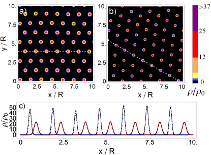
Figure 5: Density functions in the steady state for the GEM-3 potential obtained by integration of Eq. (12) with the pseudo-spectral method. a) $\tilde{D}=0.06$ b) $\tilde{D}=0.03$. Figure c) is the density $\rho$ along the white dotted lines shown on figures a) and b) (red and blue squares respectively). The black curves correspond to a fit by a sum of Gaussian functions.

III.2 Linear stability analysis

It is straightforward to check that any constant density function is a solution of the deterministic Dean equation. We can thus perform a linear stability analysis around a homogeneous solution $\rho({\bf x})=\rho_{0}$. In our dimensionless units all of them are represented by $\rho_{0}=1$. We consider a small harmonic perturbation of dimensionless wavenumber ${\bf k}=\textbf{q}R$, $\rho({\bf x},t)=1+\delta\rho({\bf x},t)$ with $\delta\rho({\bf x},t)=\exp{(\lambda t+i{\bf k}\cdot{\bf x})}$. Introducing in (12) and linearizing we find the following growth rate:

$$\lambda(k)=-k^{2}\left[\tilde{D}+\hat{v}(k)\right]\ ,$$ (13)

with $\hat{v}(k)$ the d-dimensional Fourier transform of the dimensionless interaction potential:

$$\hat{v}({\bf k})=\int\tilde{v}({\bf x})e^{-i{\bf k}\cdot{\bf x}}d{\bf x}\ .$$ (14)

Note that because $\tilde{v}({\bf x})$ depends only on the modulus $r$ of ${\bf x}$, $\tilde{v}({\bf x})=\tilde{v}(r)$, the same is valid for $\hat{v}$: $\hat{v}({\bf k})=\hat{v}(k)$, with $k=|{\bf k}|$. Eq.( 13) is the same in any dimension $d$, but the Fourier transform $\hat{v}(k)$ will be different for different $d$.

Figure 6 shows $\lambda(k)$ for several potentials and parameters, in 1d and 2d. This growth rate explains why we never observed patterns with a GEM-1 potential: since its Fourier components are always positive, the growth rates $\lambda(k)$ are always negative and the homogeneous state always stable. This can be generalized to any GEM-$\alpha$ potential with $\alpha<2$ Bochner1937 ; Likos2007 . Also, Eq.(13) gives us a precise condition for the onset of patterns when $\hat{v}(k)$ is negative in some range of $k$: the homogeneous state is stable only if we have

$$\tilde{D}>\tilde{D}_{c}=-\hat{v}_{1}=|\hat{v}_{1}|\ ,$$ (15)

where $\hat{v}_{1}\equiv\hat{v}(k_{c})$ and $k_{c}$ is the wavelength corresponding to the maximum growth rate. The values of $\hat{v}_{1}$ are reported in Table 1 for several types of GEM-$\alpha$ potentials. For example with $\alpha=3$, we obtain $\tilde{D}_{c}\approx 0.1017$ in 1d and $\tilde{D}_{c}\approx 0.0823$ in 2d. Note that in Fig.  3 c), the transition threshold seems to be higher with $\tilde{D}_{c}\approx 0.1$. We will see in section III.5 that this is due to the subcritical nature of the transition. Finally, the intercluster distance $c=a/R$ always corresponds to a wavelength $k=2\pi/c$ close to $k_{c}$ as can be seen in Table 1 and such as $\lambda(k)\geq 0$, indicating that the steady-state pattern is selected by the instability.

1d
$\alpha$ $\tilde{D}_{c}=-\hat{v}_{1}$ $10^{2}~{}\hat{v}_{2}$ $k_{c}=q_{c}R$ $c=a/R$ $v^{\prime\prime}(c)$ 3 0.1017 $-0.1108$ 4.5513 1.3805 1.7573 4 0.1873 $0.5767$ 4.5918 1.3683 2.4787 8 0.3326 $4.3699$ 4.6519 1.3507 0.0614

2d
$\alpha$ $\tilde{D}_{c}=-\hat{v}_{1}$ $10^{4}~{}\hat{v}_{2}$ $10^{4}~{}\hat{v}_{12}$ $k_{c}=q_{c}R$ $c=a/R$ $v^{\prime\prime}(c)$ 3 0.0823 $-5.4727$ $5.6030$ 5.0 1.4425 1.5068 4 0.1568 $-7.4218$ $139.04$ 5.1 1.3645 2.5269 8 0.2939 $-94.321$ $813.35$ 5.2 1.2671 1.9878

Table 1: Important values of the Fourier transform of some GEM-$\alpha$ potentials in 1d and 2d. Intercluster distance $a$ is estimated from the location $q_{c}$ of the maximum growth rate as $a=2\pi/q_{c}$, so that $c=2\pi/k_{c}$

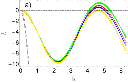
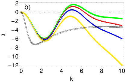
Figure 6: Growth rates, from Eq. (13) a) 1d. GEM-3 potential with $\tilde{D}=0.075$ (green squares), $0.084$ (red triangles), $0.09$ (blue diamonds) and $0.1005$ (yellow disks) and GEM-1 potential with $\tilde{D}=0.075$ (black squares). b) 2d. GEM-3 potential with $\tilde{D}=0.015$ (green squares), $0.03$ (red triangles), $0.06$ (blue diamonds) and $0.12$ (yellow disks) and GEM-1 potential with $\tilde{D}=0.015$ (black squares).

III.3 The physical mechanism: effective cluster interactions

The linear stability analysis provides a clear mathematical explanation of the instability of the homogeneous state, but it continues to be counterintuitive to observe clusters composed of very close particles despite they repel each other. In fact, for hard spheres the solid state is a crystal of individual particles, not clusters of them. The reason for cluster formation is that, despite there is intracluster repulsion, the particles are also repelled by the particles in the neighboring clusters. For interactions of the GEM-$\alpha$ type with $\alpha>2$ the combined repulsion each particle feels from the ones in neighboring clusters is larger than the repulsion from the same-cluster particles. We can see this from the following argument, which also gives us a way to estimate analytically the cluster width for small $\tilde{D}$.

Equation (12) can be written as a particle-conservation equation:

$$\partial_{t}\rho({\bf x},t)=-\nabla\cdot{\bf J}({\bf x},t)\ ,$$ (16)

with the particle-flux vector given by

$${\bf J}({\bf x},t)=-\rho({\bf x},t)\int d{\bf x}^{\prime}\nabla\tilde{v}({\bf x}-{\bf x}^{\prime})\rho({\bf x}^{\prime},t)-\tilde{D}\nabla\rho({\bf x},t)\ .$$ (17)

We consider zero-flux steady state solutions of Eq. (12), i.e. solutions with $\textbf{J}=\textbf{0}$ in (17):

$$\rho({\bf x})\int d{\bf y}\nabla\tilde{v}({\bf x}-{\bf y})\rho({\bf y})=-\tilde{D}\nabla\rho({\bf x}),$$

which, after integration gives us

$$\rho({\bf x})=\exp\left[\frac{1}{\tilde{D}}\left(\mu-\int d{\bf y}\,\rho({\bf y})\tilde{v}({\bf x}-{\bf y})\right)\right].$$ (18)

$\mu$ is an integration constant, to be fixed by the normalization of $\rho$, and that can be identified with a chemical potential. We consider Eq. (18) as an iterative procedure to obtain the steady configuration: by substituting in the right-hand-side of the equation a first approximation to the density, the left-hand-side will give an improved one. In the limit of $\tilde{D}\to 0$, for which the density becomes a periodic arrangement of narrow clusters, a sensible first approximation would be an array of delta-function clusters. In the one-dimensional case this is

$$\rho(y)\approx N_{p}\sum_{n}\delta(y-nc)\ .$$ (19)

The sum over $n$ is over all clusters in the system, and the origin of coordinates is such that there is a cluster at $y=0$. $c$ is the intercluster distance. It would be close to the most unstable wavelength, i.e. $c\approx 2\pi/k_{c}$. $N_{p}$ is the number of particles contained in each cluster. For identical clusters it is $N_{p}=Nc/L=c$, where the last inequality arises since we are using units such that $\rho_{0}=R=1$.

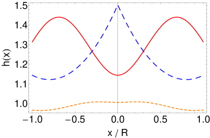
Figure 7: Effective potential $h(x)$. Solid: GEM-3 potential, with intercluster distance $c=a/R=1.38$, which is (see Table 1) the periodicity given by the linear stability analysis. Dashed: $h(x)$ for GEM-1. We use the same value $c=1.38$, although the peak at the origin is independent of the intercluster separation. Dotted: $h(x)$ for the GEM-3 potential but for a larger intercluster separation $c=1.8$.

Inserting this first approximation back into Eq. (18) we obtain the improved approximation:

$$\rho(x)\approx\exp\left[\frac{1}{\tilde{D}}\left(\mu-N_{p}\sum_{n}\tilde{v}(x-nc)\right)\right].$$ (20)

The GEM-$\alpha$ functions $\tilde{v}(x)$ are rapidly decreasing towards zero as soon as $x>R=1$. Then, at each particular location $x$, it is a good approximation to take into account only the contributions to the sum from the closest cluster and from their two neighbors, provided cluster separation is larger than $R$. For example, if we want to approximate the density close to $x\approx 0$ we can consider the terms with $n=0$ and $n=\pm 1$ in (20):

$$\rho(x\approx 0)\approx e^{\frac{\mu}{\tilde{D}}}\exp\left(-\frac{N_{p}}{\tilde{D}}h(x)\right)\ ,$$ (21)

where

$$h(x)\equiv\tilde{v}(x)+\tilde{v}(x+c)+\tilde{v}(x-c)\ .$$ (22)

The shape of the cluster close to the origin is determined by the function $h(x)$ which acts as an effective potential felt by a test particle at position $x$. $h(x)$ combines the repulsion from the particles in the cluster at the origin, $\tilde{v}(x)$, with the repulsion from the particles in the neighboring ones $\tilde{v}(x\pm c)$. If the resulting $h(x)$ has a minimum at the origin our assumption of a narrow cluster there would be justified. On the contrary, a maximum of $h(x)$ at the origin implies that the internal repulsion dominates, our approximations (19) and (20) would be inadequate, and the iteration procedure does not converge to a steady configuration consisting on well separated clusters. Figure 7 shows the function $h(x)$ for various GEM-$\alpha$ potentials. A maximum at the origin and then lack of convergence to localized clusters occurs when $\alpha<2$ (see Fig.  7 for GEM-1). A change of behavior at the origin occurs precisely at $\alpha=2$. This can be seen by expanding $h(x)$ close to the origin: Using $\tilde{v}(x)=\exp(-|x|^{\alpha})\approx 1-|x|^{\alpha}+\ldots$ and that $\tilde{v}(x)$ is analytic at any $x\neq 0$ we find

$$h(x)\approx 1+2\tilde{v}(c)+\tilde{v}^{\prime\prime}(c)x^{2}-|x|^{\alpha}+\ldots$$ (23)

If $\alpha<2$ the dominant term is $-|x|^{\alpha}$ which gives a maximum at the origin and then Eq. (20) does not give localized clusters at the intended positions. When $\alpha>2$ the quadratic term dominates at small $x$ and the maximum or minimum character of $h(x)$ at the origin is determined by the second derivative or curvature $\tilde{v}^{\prime\prime}(c)$, which for the GEM-$\alpha$ potential is:

$$\tilde{v}^{\prime\prime}(c)=c^{\alpha-2}\alpha(1-\alpha+\alpha c^{\alpha})e^{-c^{\alpha}}\ .$$ (24)

For very small intercluster separation $c$, $v^{\prime\prime}(c)$ becomes negative and then the situation is similar to $\alpha<2$. But in the tail of the potential, i.e. if $c\gtrsim 1$ (as when cluster distance is given by the linear instability, see Table 1) this curvature is always positive and the iterative procedure will converge (if $\tilde{D}$ is small) to a steady solution made of localized clusters. $h(x)$ for GEM-3 and intercluster distance $c$ given by the linear stability analysis is plotted in Fig.  7, showing a clear confining character at the origin. Values of the linearly-determined $c$ and of $v^{\prime\prime}(c)$ for other values of $\alpha$ are in Table 1. When the intercluster distance is too large, however, the influence of the neighboring clusters becomes weaker. As shown in Fig.  7 for a large $c=1.8$, the minimum character of the origin is preserved, but the minimum is very shallow and the absolute minima are not there, but at lateral positions. Thus, the iterative procedure starting with the ansatz Eq. (19) will not converge to a proper steady solution neither in this case. This gives a range of periodicities (roughly $R\lesssim a\lesssim 2R$) for which intercluster repulsion under GEM-$\alpha$ potentials with $\alpha>2$ lead to localized clusters despite the internal repulsion existing in all of them.

We have focused in this section on the one-dimensional case, but it is easy to see that the general ideas and mechanisms are valid in any dimension $d$ and in fact we use them in the next subsection to obtain quantitative expressions for cluster width and shape in 1d and in 2d.

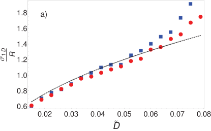
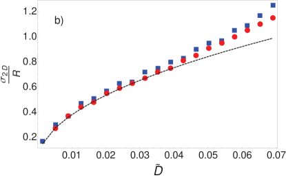
Figure 8: Clusters width as a function of $\tilde{D}$ for a GEM-3 potential. Red circles: from the steady density solution of the DK equation. Blue squares: from a coarse-grained density in particle simulations. In both cases, the Gaussian fit was made focusing on the top of the clusters. a) One-dimensional case. Dashed black line is Eq. (27). b) Two-dimensional case. Dashed black line is Eq. (33). The intercluster distance $c$ used in the analytical formula was obtained from the position of the second peak of the radial distribution function $g^{(2)}(r)$ (see Fig.  3 a)), which gives a result slightly better than using the linear instability value $2\pi/k_{c}$. In the particle case the coarse graining in 1d and in 2d was done as in Figs. 1 and 2 respectively.

III.4 Shape and width of clusters

The above arguments shed additional insight on the results of the linear stability analysis: homogeneous distributions become unstable against pattern formation of periodicity precisely in the range which allows the particles to remain confined in well-localized clusters. All the explanations rely on having narrow clusters, which is only justified if $\tilde{D}$ remains sufficiently small. In this limit (and for $\alpha>2$), expressions (21)-(23), valid for $x\approx 0$, can be used to provide an estimation of the central cluster shape and width. In one dimension we have

$$\rho(x)\approx e^{\frac{\mu-N_{p}(1+2\tilde{v}(c))}{\tilde{D}}}e^{-\frac{N_{p}}{\tilde{D}}\tilde{v}^{\prime\prime}(c)x^{2}}\equiv\frac{N_{p}}{\sqrt{2\pi\sigma^{2}}}e^{-\frac{x^{2}}{2\sigma^{2}}}\ ,$$ (25)

so that each cluster can be approximated by a Gaussian of width

$$\sigma=\sqrt{\frac{\tilde{D}}{2N_{p}\tilde{v}^{\prime\prime}(c)}}\ .$$ (26)

Denoting $\sigma_{1D}$ this width in the original unscaled units, and using that $N_{p}=c=a/R$ this expression can be written as:

$$\frac{\sigma_{1D}}{R}=\sqrt{\frac{D}{2\epsilon\rho_{0}a\tilde{v}^{\prime\prime}(c)}}$$ (27)

Figure 8 a) compares this formula with the width obtained from 1d numerical simulations of the particle system and of the DK equation. We see that for the lowest values of $\tilde{D}$, the agreement is really good in both cases. For higher values of $\tilde{D}$, our calculations tend to underestimate the width of the clusters. This is coherent with our hypothesis as we assumed very small values of $\tilde{D}$ and well separated clusters.

In this $\tilde{D}\rightarrow 0$ limit the full density, according to Eq. (20) is an array of Gaussian peaks:

$$\rho(x)\approx\frac{N_{p}}{\sqrt{2\pi\sigma^{2}}}\sum_{n}e^{-\frac{(x-nc)^{2}}{2\sigma^{2}}}\ .$$ (28)

The maximum (peak) value of the density is then (using $N_{p}=c$)

$$\rho_{max}=\frac{1}{\sqrt{2\pi}}\frac{c}{\sigma}\ ,$$ (29)

or in terms of unscaled variables (and $a=cR$):

$$\frac{\rho_{max}}{\rho_{0}}=\frac{1}{\sqrt{2\pi}}\frac{a}{\sigma_{1D}}\ .$$ (30)

This expression is plotted in Fig.  9 as a dashed line, and compared with the numerically obtained 1d steady solution of the DK equation and with particle simulations. As expected, it becomes accurate when $\tilde{D}\rightarrow 0$ but becomes increasingly worse when $\tilde{D}$ approaches the transition point. This opposite regime will be discussed in the next subsection.

All the previous calculations can be essentially repeated in 2d. The only major difference is the starting point as we now have to replace Eq. (19) by a hexagonal lattice of delta functions:

$$\rho({\bf y})\approx N_{p}\sum_{n}\sum_{m}\delta({\bf y}+n\boldsymbol{c}_{1}+m\boldsymbol{c}_{2}),$$ (31)

where $\boldsymbol{c}_{1}$ and $\boldsymbol{c}_{2}$ are two vectors of norm $c$ necessary to generate the hexagonal patterns. Following the same method as in one dimension, we find that the clusters have once again a Gaussian shape with width $\sigma$ given by

$$\sigma=\sqrt{\frac{2\tilde{D}}{3\sqrt{3}\alpha^{2}c^{\alpha}(c^{\alpha}-1)e^{-c^{\alpha}}}}\ ,$$ (32)

which gives us in unscaled units

$$\frac{\sigma_{2D}}{R}=\sqrt{\frac{2D}{\epsilon\rho_{0}R^{2}3\sqrt{3}\alpha^{2}c^{\alpha}(c^{\alpha}-1)e^{-c^{\alpha}}}}\ .$$ (33)

This formula is compared with numerical measurements in Fig.  8 b) for $\alpha=3$. The agreement with particle and DK data is once again very good as long as the value of $\tilde{D}$ is small enough.

III.5 The neighborhood of the transition point

In the previous subsection we obtained an accurate description of the patterns formed at small $\tilde{D}$. At the same time the theoretical arguments to obtain it gave useful insight into the mechanisms of the cluster crystal formation. But this description became inaccurate as $\tilde{D}$ increased, and can not describe the neighborhood of the instability point. Here we focus on that regime, using weakly nonlinear expansions Walgraef2012 close to the bifurcation point $\tilde{D}_{c}=-\hat{v}_{1}=|\hat{v}_{1}|$. Although this type of description is appropriate for solutions of the deterministic DK equation, it should be recognized that fluctuations effects tend to be noticeable close to instability points, and then it is not guaranteed that the expressions obtained in the present subsection would be accurate for the stochastic particle system.

Figure 9: For each value of $\tilde{D}$ the maximum and the minimum value of the steady density in 1d for $\alpha=3$ are plotted. The inset gives an enlargement of the bifurcation region. Squares ($\Box$): values from direct numerical simulation of the DK equation. *, $\times$ and +: values from a coarse-grained density in particle simulations at $\rho_{0}=1000$, $1500$ and $2000$ respectively ($R=0.1$, $\epsilon=0.0333$). Solid line: the weakly nonlinear approximation Eq. (34), including up to the second harmonic. Dotted line: only the first harmonic term in Eq. (34). Dashed line: the maximum of the pattern as given by the Gaussian approximation, Eq. (30). In the particle case the coarse graining was done as in Fig. (1).

We start with the 1d case. Details of the calculations are in the Appendix. We use a weakly nonlinear expansion in powers of a small parameter which turns out to be the square root of the distance to the bifurcation point, $\sqrt{|\hat{v}_{1}|-\tilde{D}}$. We obtain an amplitude equation describing the dynamics close to the bifurcation. From it, the steady periodic solution up to second order in the small parameter reads

$$\rho_{st}(x)=1+K(|\hat{v}_{1}|-\tilde{D})^{1/2}\cos(k_{c}x)+\frac{2(|\hat{v}_{1}|-\tilde{D})}{2\hat{v}_{2}+|\hat{v}_{1}|}\cos(2k_{c}x)\ ,$$ (34)

where $\hat{v}_{2}=\hat{v}(2k_{c})$,

$$K\equiv 2\left(\frac{2(1+\hat{v}_{2}/|\hat{v}_{1}|)}{2\hat{v}_{2}+|\hat{v}_{1}|}\right)^{1/2}\ ,$$ (35)

and the pattern position has been chosen to be such that there is a maximum at $x=0$. Values of $\hat{v}_{1}$ and $\hat{v}_{2}$ for different values of $\alpha>2$ are in Table 1. Figure 9 compares this expression with maximum and minimum values of the density distribution for $\alpha=3$, numerically obtained from the 1d DK equation and from particle simulations. It is seen that the approximation including only the first harmonic is accurate just very close to the instability point and that the range of validity is improved by including the second-order term. Note that the continuous character of the bifurcation in the DK equation is correctly predicted by the theoretical formula. For small values of $\tilde{D}$ the agreement becomes rather poor, as expected, but the maximum values of the density can then be predicted by the Gaussian approximation and Eq. (30). It is also worth mentioning that, in most of the $\tilde{D}$ range, proper scaling is observed when plotting the maximum and minimum values of the coarse-graining particle density in terms of the dimensionless quantities identified from the deterministic DK equation, and that only small differences between the DK density and the one obtained from particle simulations are observed. This confirms that neglecting noise, which has allowed us to get analytic insight, is a good approximation in most of the parameter range. The exception is the neighborhood of the bifurcation point of the DK equation since, as commented before, we do not expect a sharp transition for the particle system in 1d. The effect of this somehow smoother transition is an apparent shifting of the critical point to smaller values of $\tilde{D}$ for particle simulations, an expected result of the presence of fluctuations. This also explains why the local density was more sinusoidal on the top right part of Fig.  1 than on Fig.  4 b): as the particle simulations are noisy, at this value of $\tilde{D}$ the system is deeper into the periodic state and further away from the transition point in the DK case.

We now turn out to two-dimensional systems. Following a similar weakly nonlinear procedure, we find the following expression for the density for $\tilde{D}$ close to $\tilde{D}_{c}$ (see details in the Appendix):

$$\rho_{st}({\bf x})=1+2\delta_{0}\left(\cos({\bf k}_{1}\cdot{\bf x})+\textrm{cyclic}\right)+\frac{\delta_{0}^{2}|\hat{v}_{1}|}{(|\hat{v}_{1}|+\hat{v}_{2})}\left(\cos(2{\bf k}_{1}\cdot{\bf x})+\textrm{cyclic}\right)+\frac{2\delta_{0}^{2}|\hat{v}_{1}|}{|\hat{v}_{1}|+\hat{v}_{12}}\left(\cos({\bf k}_{12}\cdot{\bf x})+\textrm{cyclic}\right)\ ,$$ (36)

where $\delta_{0}$ is, up to second order, a positive solution of

$$\frac{D-|\hat{v}_{1}|}{|\hat{v}_{1}|}=\delta_{0}-\delta_{0}^{2}\left(\frac{|\hat{v}_{1}|+2\hat{v}_{2}}{2(|\hat{v}_{1}|+\hat{v}_{2})}+\frac{|\hat{v}_{1}|+3\hat{v}_{12}}{|\hat{v}_{1}|+\hat{v}_{12}}\right)\ .$$ (37)

The terms in ‘cyclic’ are cosines similar to the ones explicitly shown but with arguments obtained by changing cyclically ($1\rightarrow 2\rightarrow 3\rightarrow 1$) the subindices of vectors ${\bf k}_{1}$ and ${\bf k}_{12}$ (which are defined in the Appendix). In this way $\rho_{st}({\bf x})$ has hexagonal symmetry, with periodicity determined by $k_{c}=|{\bf k}_{1}|$. Figure 10 shows the behavior with respect to $\tilde{D}$ of the maximum value of $\rho_{st}/\rho_{0}$ according to Eqs. (36) and (37) and compares them with the numerical results of the 2d DK equation. Equation (37), quadratic in $\delta_{0}$, gives two different branches for $\delta_{0}$ in a range of $\tilde{D}$, coalescing and disappearing at a turning point. Only the upper branch is stable. Then, the bifurcation is subcritical in 2d, with two stable steady densities existing near the critical point, the homogeneous $\rho=\rho_{0}$ and the hexagonal density with amplitude determined by the upper-branch solution of (37). In agreement with the analytic approach, a hysteretic behavior is clearly visible in the DK simulations. The upper branch corresponds to the hexagonal pattern that discontinuously becomes homogeneous when increasing $\tilde{D}$ beyond $\tilde{D}\approx 0.0957$. The quantitative agreement between simulations and theory is rather poor as Eq. (36) systematically underestimates the density peaks. This is a consequence of the theory being an expansion in the neighborhood of the point $(\tilde{D}=\tilde{D}_{c},\rho/\rho_{0}=1)$, whereas the interesting upper branch of the density its quite far from there. For smaller values of $\tilde{D}$ the 2d Gaussian approach gives a better description, as confirmed by Fig. 8b. We note however that the turning point predicted from Eqs. (36) and (37) gives a reasonable approximation to the numerical location of the jump to homogeneous density in the DK case. Although it is out of the scope of the present paper to elucidate if the sharp jump in the maximum of the structure factor in the particle system (see Fig. 3 c) is actually continuous or discontinuous, indicating a continuous or discontinuous melting, we note that the discontinuous jump occurring in the deterministic DK steady solution gives a good approximation ($\tilde{D}\approx 0.0957$, a value of $\tilde{D}$ larger than the linear $\tilde{D}_{c}=|\hat{v}_{1}|$) for the location of the particle transition, as seen in Fig. 3 c.

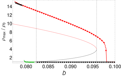
Figure 10: Maximum value $\rho_{max}/\rho_{0}$ of the steady density solution of the DK equation in 2d for $\alpha=3$. We start from $\tilde{D}=0.077$, slowly increase it up to $\tilde{D}=0.102$ (red disks) and then slowly decrease $\tilde{D}$ back to its initial value (black squares and green diamonds). The plot clearly highlights a hysteretical behavior. The green diamonds indicate that $\rho_{max}/\rho_{0}$ remains close to $1$ during the times accessible to our simulation, but clearly increasing, even if very slowly. For the black squares in the lower branch $\rho_{max}/\rho_{0}$ is observed to decrease towards 1. Thus the behavior is consistent with the theoretical threshold for stability of the homogeneous solution ($\tilde{D}\approx 0.0823$, see Table 1, marked with a dotted vertical line) and we expect the green diamonds to reach the upper density branch in a sufficiently long simulation. The thin undotted lines give the theoretical prediction for $\rho_{max}$ from Eq. (36): two branches, giving the upper one a prediction for the amplitude of the stable hexagonal density. The right dotted vertical line indicates its turning point.

IV Dynamics with soft attractive interactions

For completeness, we study in this section the case opposite to the previous repulsive situation, i.e. particles interacting via purely attractive forces. The relevance of this problem is reflected in many fields of physics or biology dealing with the problem of particles attracting each other Topaz2006 ; Chavanis2008a .

Figure 11: Dynamics of 600 Brownian particles with attractive interactions in a periodic domain of size $L=3$, so that $\rho_{0}=200$. $\epsilon=-0.33$, $R=0.1$, and $D=3.96\times 10^{-3}$, so that $\tilde{D}=6\times 10^{-4}$. a) GEM-1 attractive potential. b) GEM-3 attractive potential.

We consider Brownian dynamics as in Eq. (3) with a potential given also by Eq. (4), but now it is attractive, so that $\epsilon<0$. The dimensionless version of the potential is $\tilde{v}({\bf x})=-\exp(-|{\bf x}|^{\alpha})$. In Fig. 11 we show a spatiotemporal plot of the 1d particle positions for both $\alpha=1$ and $\alpha=3$, starting from random initial conditions. Despite the visible differences between the two cases, the qualitative features of the dynamics are the same: in both situations clusters periodically spaced emerge at short times. Then clusters attract each other and coalesce. In this coarsening process the pattern periodicity increases, although at late times cluster separation becomes progressively more irregular and each cluster behaves essentially as isolated. As in the repulsive case, if $\tilde{D}$ is sufficiently large, cluster formation does not occur. The same phenomenology is observed in 2d, and this is also the behavior of the solutions of the 1d and 2d DK equation with attractive potential. Figure  12 displays 2d late time configurations for both the particle dynamics and the DK description. The figure shows also that the shape of the clusters is approximately Gaussian.

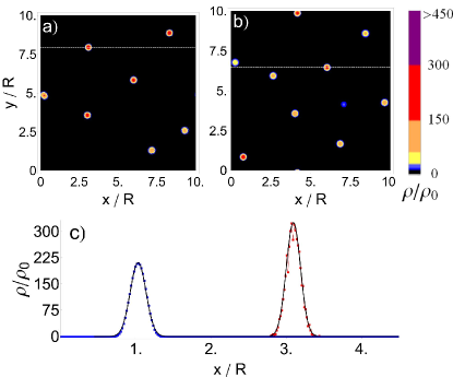
Figure 12: Density functions at large times for the attractive GEM-3 potential and $\tilde{D}=0.0975$. a) Coarse-grained density of particle simulations. $R=0.1$, $\epsilon=0.0333$, $N=2000$, $L=1$ (so that $\rho_{0}=2000$). The coarse graining procedure is as in Fig. 2. b) Integration of Eq. (12) with the pseudo-spectral method. Figure c) is the density $\rho/\rho_{0}$ along the white dashed lines shown on Figs. a) and b) (red and blue squares respectively), shifted for convenience. The black curves correspond to a fit by a sum of Gaussian functions.

Because of the attraction one would expect a collapse of all the particles in a single cluster. In fact, this is what happens but at extremely long times. The clustering is a consequence of particle’s attraction, and several aggregates remain if the attraction is weak and the clusters are distant enough from each other. In the case of the noiseless DK equation, if the interaction has a strictly finite range, clusters located farther apart than this range do not coalesce and the pattern would remain stationary.

A main difference with the repulsive case is that the cluster patterns appear for any value of $\alpha$. This can be easily explained from the linear stability analysis of the homogeneous density. The growth rate of perturbations remains the same as in Eq. (13) but now, since $\epsilon<0$ the Fourier transform of the potential will have negative values independently of $\alpha$. Figure 13 shows the growth rate $\lambda(k)$ for some parameter values. As before, for large values of $\tilde{D}$, $\lambda(k)<0$ for all $k$, so that no instability to cluster formation will occur on the homogeneous density.

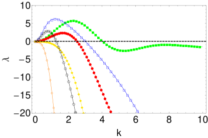
Figure 13: Growth rate (Eq. (13)) for attractive GEM-3 and GEM-1 potentials (full and empty symbols respectively). For GEM-3: $\tilde{D}=0.015$ (green squares), $0.9$ (red disks) and $3$ (yellow diamonds). For GEM-1: $\tilde{D}=0.6$ (blue squares), $4.5$ (black circles) and $21$ (orange diamonds).

V Summary and conclusions

We have analyzed in detail the properties of a system of interacting Brownian particles in the presence of a soft-core repulsive two-body potential. The relevant result is that in a range of parameters, despite the repulsion, the particles aggregate in clusters that periodically arrange in space. We have studied the system at two descriptive levels: the microscopic particle dynamics, and the DK equation for the coarse-grained density of particles. By considering the deterministic version of the DK equation we have obtained the condition for pattern formation, which is that the Fourier transform of the potential must have negative values, and when this is the case, the diffusion coefficient has to be small enough. When diffusion is small the single clusters have a Gaussian shape maintained by the interplay between repulsion between close particles and diffusion, which tend to increase cluster width, and repulsion from particles in neighboring clusters, which tends to narrow the clusters. In addition to clearly identifying the mechanisms involved, our approach based on the deterministic DK equation has allowed the derivation of analytical expressions for cluster width and height in 1d and in 2d which are accurate for small diffusion. The bifurcation behavior of the steady density has also been analyzed close to the onset of instability of the homogeneous state, obtaining approximations for the periodic density patterns formed in 1d and 2d. Finally, the situation in which the particles interact attractively has been briefly considered, obtaining also situations of cluster formation. Similarities and differences with the repulsive case have been commented.

The consideration of low dimensions (one and two) and the restriction to a deterministic approach in which pattern formation techniques become powerful has allowed us to gain insight into this counterintuitive clustering instability in which particle repulsion leads to clustering. We close by noting the strong formal analogies, including the condition for linear instability, with the situation of cluster formation in models of population dynamics, with non-conserved number of particles, in which the repulsive interaction is replaced by a negative influence of the individuals onto the growth of others, i.e. competitive interaction Hernandez2004 ; MartinezGarcia2013 ; Hernandez2014 . The phenomenon studied here i.e. the formation of crystals of clusters induced by an instability of the density in the presence of repulsive or competitive feedbacks is thus very general and could be found in many other kinds of systems.

Appendix: Weakly nonlinear analysis close to instability points

We want to obtain an equation for the deviation of the solution of the Dean equation with respect to the homogenous solution $\rho_{0}$ close to its instability threshold. Using dimensionless variables so that $\rho_{0}=1$ the equation for $\delta({\bf x},t)=\rho({\bf x},t)-1$ is

$$\dot{\delta}({\bf x},t)=\tilde{D}\nabla^{2}\delta({\bf x},t)+\textrm{G}\delta({\bf x},t)+\nabla\cdot\left(\delta({\bf x},t){\bf H}\delta({\bf x},t)\right)\ .$$ (38)

We have defined the operators ${\bf H}$ and G as

$${\bf H}f({\bf x})=\int\nabla\tilde{v}({\bf x}-{\bf x}^{\prime})f({\bf x}^{\prime})d{\bf x}^{\prime}$$ (39)

and

$$\textrm{G}f({\bf x})=\int\nabla^{2}\tilde{v}({\bf x}-{\bf x}^{\prime})f({\bf x}^{\prime})d{\bf x}^{\prime}\ .$$ (40)

We note that

$${\bf H}e^{i{\bf k}\cdot{\bf x}}=i{\bf k}\hat{v}(-{\bf k})e^{i{\bf k}\cdot{\bf x}}=i{\bf k}\hat{v}(k)e^{i{\bf k}\cdot{\bf x}}\ ,$$ (41)

where the last equality arises because $\hat{v}({\bf k})$ depends only on the modulus of ${\bf k}$: $\hat{v}({\bf k})=\hat{v}(k)$, and

$$\textrm{G}e^{i{\bf k}\cdot{\bf x}}=-k^{2}\hat{v}(k)e^{i{\bf k}\cdot{\bf x}}\ .$$ (42)

The homogeneous solution $\delta=0$ becomes unstable for $\alpha>2$, for which $\hat{v}({\bf k})$ has negative Fourier components, and $\tilde{D}<-\hat{v}(k_{c})$. We use the notation $\hat{v}_{1}=\hat{v}(k_{c})$ and $\hat{v}_{2}=\hat{v}(2k_{c})$ and introduce the expansions

$$\tilde{D} = \tilde{D}_{c}+a_{1}\eta+a_{2}\eta^{2}+a_{3}\eta^{3}+\ldots$$ (43)

$$\delta({\bf x},t) = 0+\eta\psi_{1}+\eta^{2}\psi_{2}+\eta^{3}\psi_{3}+\ldots$$ (44)

where $\tilde{D}_{c}=-\hat{v}_{1}=|\hat{v}_{1}|$, $\psi_{i}=\psi_{i}({\bf x},T,...)$, $T=\eta^{2}t+\ldots$.

We obtain

$${\cal O}(\eta): \textrm{L}_{c}\psi_{1} =0$$ (45)

$${\cal O}(\eta^{2}): \textrm{L}_{c}\psi_{2} =-a_{1}\nabla^{2}\psi_{1}-\nabla\cdot\left(\psi_{1}{\bf H}\psi_{1}\right)$$ (46)

$${\cal O}(\eta^{3}): \textrm{L}_{c}\psi_{3} =\partial_{T}\psi_{1}-a_{1}\nabla^{2}\psi_{2}-a_{2}\nabla^{2}\psi_{1}$$ (47)

$$-\nabla\cdot\left(\psi_{1}{\bf H}\psi_{2}\right)-\nabla\cdot\left(\psi_{2}{\bf H}\psi_{1}\right)\ ,$$

where the critical operator is $\textrm{L}_{c}=\tilde{D}_{c}\nabla^{2}+\textrm{G}$.

The general solution of Eq. (45) is

$$\psi_{1}=\sum_{{\bf k}}A_{\bf k}(T)e^{i{\bf k}\cdot{\bf x}}\ ,$$ (48)

where the sum is over wavevectors with the critical modulus $|{\bf k}|=k_{c}$.

We start with the one-dimensional case, for which Eq. (48) reduces to

$$\psi_{1}=A(T)e^{ik_{c}x}+\textrm{cc}\ .$$ (49)

cc means complex conjugate. Substituting in Eq. (46):

$$\textrm{L}_{c}\psi_{2}=a_{1}k_{c}^{2}A(T)e^{ik_{c}x}+2k_{c}^{2}A(T)^{2}\hat{v}_{1}e^{2ik_{c}x}+\textrm{cc}\ .$$ (50)

Fredholm theorem requires $a_{1}=0$ to avoid resonances, and then, neglecting the solution of the homogeneous solution, $\psi_{2}$ is given by

$$\psi_{2}=\frac{A(T)^{2}e^{2ik_{c}x}}{2\left(1-\frac{\hat{v}_{2}}{\hat{v}_{1}}\right)}+\textrm{cc}\equiv B(T)e^{2ik_{c}x}+\textrm{cc}\ .$$ (51)

Going to the next order, Eq. (47):

$$\textrm{L}_{c}\psi_{3}=e^{ik_{c}x}\left(\partial_{T}A(T)+a_{2}k_{c}^{2}A\right.$$ (52)

$$+ \left.k_{c}^{2}BA^{*}\left[2\hat{v}_{2}-\hat{v}_{1}\right]\right)+\textrm{cc}+{\cal O}(e^{3ik_{c}x})\ .$$

Again, elimination of resonances requires

$$\partial_{T}A = -a_{2}k_{c}^{2}A-k_{c}^{2}A^{*}B\left(2\hat{v}_{2}-\hat{v}_{1}\right)$$ (53)

$$= -a_{2}k_{c}^{2}A-k_{c}^{2}\frac{2\hat{v}_{2}-\hat{v}_{1}}{2\left(1-\frac{\hat{v}_{2}}{\hat{v}_{1}}\right)}|A|^{2}A\ ,$$

which is the amplitude equation describing the dynamics at $\tilde{D}\approx\tilde{D}_{c}$. The steady solution is

$$|A_{st}|^{2}=\frac{-2a_{2}\left(1-\hat{v}_{2}/\hat{v}_{1}\right)}{2\hat{v}_{2}-\hat{v}_{1}}\ .$$ (54)

Using the expansion (43):

$$\eta=\sqrt{\frac{\tilde{D}_{c}-\tilde{D}}{-a_{2}}}+\ldots$$ (55)

the expansion (44) for the steady state becomes

$$\delta(x)=\left(\frac{(\tilde{D}_{c}-\tilde{D})2(1-\hat{v}_{2}/\hat{v}_{1})}{2\hat{v}_{2}-\hat{v}_{1}}\right)e^{ik_{c}x+i\phi}+\textrm{cc}$$

$$+\frac{\tilde{D}_{c}-\tilde{D}}{-a_{2}}\psi_{2}(x)+\ldots$$ (56)

$\phi$ is the (arbitrary) phase of $A_{st}$, fixing the position of the pattern, and that in the following we take $\phi=0$. Finally, using that $D_{c}=-\hat{v}_{1}=|\hat{v}_{1}|$ we find expression (34) in the main text. Given the signs in Eq. (56), we have a supercritical bifurcation from the homogeneous state to a periodic array of clusters when $\tilde{D}$ is reduced below $\tilde{D}_{c}$.

The procedure can be repeated in two dimensions. For simplicity we focus directly on the steady solutions, so that the term $\partial_{T}\psi_{1}$ is absent from Eq. (47). The solution of Eq. (45) with hexagonal symmetry is

$$\psi_{1}=\sum_{r=1,2,3}A_{r}e^{i{\bf k}_{r}\cdot{\bf x}}+\textrm{cc}\ ,$$ (57)

where ${\bf k}_{r}$, $r=1,2,3$ are three wavevectors of modulus $k_{c}$ and oriented 120 degrees apart. Together with the other three wavevectors contained in the complex conjugate (cc) terms, they complete the hexagonal platform that generates the hexagonal pattern. We note that ${\bf k}_{1}+{\bf k}_{2}=-{\bf k}_{3}$, ${\bf k}_{2}+{\bf k}_{3}=-{\bf k}_{1}$, and ${\bf k}_{3}+{\bf k}_{1}=-{\bf k}_{2}$. Other vectors that appear in the nonlinear expansion are ${\bf k}_{12}={\bf k}_{1}-{\bf k}_{2}$, ${\bf k}_{23}={\bf k}_{2}-{\bf k}_{3}$ and ${\bf k}_{31}={\bf k}_{3}-{\bf k}_{1}$, all of modulus $k_{12}=\sqrt{3}k_{c}$. We define $\hat{v}_{12}\equiv\hat{v}(k_{12})$.

Introducing (57) into the second order Eq. (46) we obtain as the conditions for eliminating the resonant terms:

$$a_{1}A_{1}+\hat{v}_{1}A_{2}^{*}A_{3}^{*}=0\ ,$$ (58)

and the other two complex equations resulting from cyclic permutation of the subindices of $A_{r}$: $1\rightarrow 2\rightarrow 3\rightarrow 1$. Choosing appropriately the origin of coordinates it is enough to solve (58) for real and equal amplitudes: $A_{r}=A$, $r=1,2,3$, so that

$$A=\frac{a_{1}}{|\hat{v}_{1}|}\ .$$ (59)

The second order equation can now be solved, giving a $\psi_{2}$ in terms of $A$ and $a_{1}$ and with spatial structure containing wavevectors $2{\bf k}_{r}$ and ${\bf k}_{rs}$, $r,s=1,2,3$. Eliminating again resonant terms from Eq. (47) and defining $\delta_{0}=\eta A$ we find the two formulas given in the main text, namely Eq. (36) and (37). There is a subcritical bifurcation from homogeneous to hexagonal density when reducing $\tilde{D}$.

References

- (1) A. J. Archer and M. Rauscher, Dynamical density functional theory for interacting Brownian particles: stochastic or deterministic?, Journal of Physics A: Mathematical and General, 37 (2004), pp. 9325—-9333.
- (2) A. J. Archer, A. M. Rucklidge, and E. Knobloch, Quasicrystalline order and a crystal-liquid state in a soft-core fluid, Phys. Rev. Lett., 111 (2013), p. 165501.
- (3) , Soft-core particles freezing to form a quasicrystal and a crystal-liquid phase, Phys. Rev. E, 92 (2015), p. 012324.
- (4) E. Ben-Jacob, I. Cohen, and H. Levine, Cooperative self-organization of microorganisms, Advances in Physics, 49 (2000), pp. 395–554.
- (5) S. Bochner, Stable laws of probability and completely monotone functions, Duke Math. J., 3 (1937), pp. 726–728.
- (6) E. Bonabeau, Agent-based Methods and techniques for simulating human systems, Proceedings of the National Academy of Sciences of the USA, 99 (2002), pp. 7280–7287.
- (7) F. Borgogno, P. D’Odorico, F. Laio, and L. Ridolfi, Mathematical models of vegetation pattern formation in ecohydrology, Reviews of Geophysics, 47 (2009), p. RG1005.
- (8) P.-H. Chavanis, Hamiltonian and Brownian systems with long-range interactions: IV. General kinetic equations from the quasilinear theory, Physica A: Statistical Mechanics and its Applications, 387 (2008), pp. 1504–1528.
- (9) D. Coslovich and A. Ikeda, Cluster and reentrant anomalies of nearly gaussian core particles, Soft Matter, 9 (2013), pp. 6786–6795.
- (10) J. A. Cuesta and A. Sánchez, General non-existence theorem for phase transitions in one-dimensional systems with short range interactions, and physical examples of such transitions, Journal of Statistical Physics, 115 (2004), pp. 869–893.
- (11) D. S. Dean, Langevin equation for the density of a system of interacting Langevin processes, Journal of Physics A: Mathematical and General, 29 (1996), pp. L613–L617.
- (12) C. W. Gardiner, Handbook of Stochastic Methods, Springer-Verlag, Berlin, 2002.
- (13) U. Gasser, Crystallization in three- and two-dimensional colloidal suspensions, Journal of Physics: Condensed Matter, 21 (2009), p. 203101.
- (14) V. Grimm and S. F. Railsback, Individual-Based Modeling and Ecology, Princeton University Press, 2005.
- (15) E. Hernández-García, E. Heinsalu, and C. López, Spatial patterns of competing random walkers, Ecological Complexity, 21 (2014), pp. 166–176.
- (16) E. Hernández-García and C. López, Clustering, advection, and patterns in a model of population dynamics with neighborhood dependent rates, Phys. Rev. E, 70 (2004), p. 016216.
- (17) K. Kawasaki, Stochastic model of slow dynamics in supercooled liquids and dense colloidal suspensions, Physica A: Statistical Mechanics and its Applications, 208 (1994), pp. 35–64.
- (18) B. Kim, K. Kawasaki, H. Jacquin, and F. van Wijland, Equilibrium dynamics of the dean-kawasaki equation: Mode-coupling theory and its extension, Phys. Rev. E, 89 (2014), p. 012150.
- (19) W. Klein, H. Gould, R. A. Ramos, I. Clejan, and A. I. Mel’cuk, Repulsive potentials, clumps and the metastable glass phase, Physica A: Statistical Mechanics and its Applications, 205 (1994), pp. 738–746.
- (20) C. N. Likos, A. Lang, M. Watzlawek, and H. Löwen, Criterion for determining clustering versus reentrant melting behavior for bounded interaction potentials, Phys. Rev. E, 63 (2001), p. 031206.
- (21) C. N. Likos, B. M. Mladek, D. Gottwald, and G. Kahl, Why do ultrasoft repulsive particles cluster and crystallize? analytical results from density-functional theory, The Journal of Chemical Physics, 126 (2007).
- (22) M. C. Marchetti, J. F. Joanny, S. Ramaswamy, T. B. Liverpool, J. Prost, M. Rao, and R. A. Simha, Hydrodynamics of soft active matter, Rev. Mod. Phys., 85 (2013), pp. 1143–1189.
- (23) U. M. B. Marconi and P. Tarazona, Dynamic density functional theory of fluids, The Journal of Chemical Physics, 110 (1999), pp. 8032–8044.
- (24) R. Martínez-García, J. M. Calabrese, E. Hernández-García, and C. López, Vegetation pattern formation in semiarid systems without facilitative mechanisms, Geophysical Research Letters, 40 (2013), pp. 6143–6147.
- (25) R. Martínez-García, J. M. Calabrese, E. Hernández-García, and C. López, Minimal mechanisms for vegetation patterns in semiarid regions, Philosophical Transactions of the Royal Society of London A: Mathematical, Physical and Engineering Sciences, 372 (2014), p. 20140068.
- (26) R. Martínez-García, C. Murgui, E. Hernández-García, and C. López, Pattern formation in populations with density-dependent movement and two interaction scales, PLoS ONE, 10 (2015), pp. 1–14.
- (27) E. Meron, Nonlinear physics of ecosystems, CRC Press, 2015.
- (28) B. M. Mladek, D. Gottwald, G. Kahl, M. Neumann, and C. N. Likos, Formation of polymorphic cluster phases for a class of models of purely repulsive soft spheres, Phys. Rev. Lett., 96 (2006), p. 045701.
- (29) B. M. Mladek, G. Kahl, and C. N. Likos, Computer assembly of cluster-forming amphiphilic dendrimers, Phys. Rev. Lett., 100 (2008), p. 028301.
- (30) T. Munakata, Liquid instability and freezing -reductive perturbation approach-, Journal of the Physical Society of Japan, 43 (1977), pp. 1723–1728.
- (31) J. D. Murray, ed., Mathematical Biology, vol. 17, Springer New York, 2004.
- (32) A. Okubo and S. A. Levin, Diffusion and Ecological Problems: Modern Perspectives, vol. 14, Springer New York, 2001.
- (33) R. Peierls, Quelques propriétés typiques des corps solides, Annales de l’institut Henri Poincaré, 5 (1935), pp. 177–222.
- (34) M. Pineda, R. Toral, and E. Hernández-García, Diffusing opinions in bounded confidence processes, The European Physical Journal D, 62 (2010), pp. 109–117.
- (35) S. Prestipino, D. Gazzillo, and N. Tasinato, Probing the existence of phase transitions in one-dimensional fluids of penetrable particles, Phys. Rev. E, 92 (2015), p. 022138.
- (36) F. Ramos, C. López, E. Hernández-García, and M. A. Muñoz, Crystallization and melting of bacteria colonies and Brownian bugs, Phys. Rev. E, 77 (2008), p. 021102.
- (37) M. Rietkerk and J. van de Koppel, Regular pattern formation in real ecosystems., Trends in Ecology and Evolution, 23 (2008), pp. 169–75.
- (38) J. Schellinck and T. White, A review of attraction and repulsion models of aggregation: Methods, findings and a discussion of model validation, Ecological Modelling, 222 (2011), pp. 1897 – 1911.
- (39) K. J. Strandburg, Two-dimensional melting, Rev. Mod. Phys., 60 (1988), pp. 161–207.
- (40) C. M. Topaz, A. L. Bertozzi, and M. A. Lewis, A nonlocal continuum model for biological aggregation, Bulletin of Mathematical Biology, 68 (2006), pp. 1601–1623.
- (41) D. Walgraef, Spatio-Temporal Pattern Formation: With Examples from Physics, Chemistry, and Materials Science, Springer-Verlag, Berlin, 2012.
- (42) M. Zu, J. Liu, H. Tong, and N. Xu, ArXiv e-print, (2016).