Strategies in seismic inference of supergranular flows on the Sun

Abstract

Observations of the solar surface reveal the presence of flows with length scales of around $35$ Mm, commonly referred to as supergranules. Inferring the sub-surface flow profile of supergranules from measurements of the surface and photospheric wavefield is an important challenge faced by helioseismology. Traditionally, the inverse problem has been approached by studying the linear response of seismic waves in a horizontally translationally invariant background to the presence of the supergranule; following an iterative approach that does not depend on horizontal translational invariance might perform better, since the misfit can be analyzed post iterations. In this work, we construct synthetic observations using a reference supergranule, and invert for the flow profile using surface measurements of travel-times of waves belonging to modal ridges $f$ (surface-gravity) and $p_{1}$ through $p_{7}$ (acoustic). We study the extent to which individual modes and their combinations contribute to infer the flow. We show that this method of non-linear iterative inversion tends to underestimate the flow velocities as well as inferring a shallower flow profile, with significant deviations from the reference supergranule near the surface. We carry out a similar analysis for a sound-speed perturbation and find that analogous near-surface deviations persist, although the iterations converge faster and more accurately. We conclude that a better approach to inversion would be to expand the supergranule profile in an appropriate basis, thereby reducing the number of parameters being inverted for and appropriately regularizing them.

1 Introduction

Helioseismology has allowed us to probe sub-surface features that are otherwise inaccessible to electromagnetic observations of the solar surface. Seismology attempts to uncover flows beneath the photosphere; such estimates act as complementary constraints on simulations of convective flows and solar dynamics. A moving background medium would advect seismic waves, and the primary impact is expected to be a shift in measured travel-time. Tracking a propagating seismic wave (Duvall et al., 1993, 1997) would therefore allow us to draw inferences about local sub-surface flows such as supergranules. Several authors (Kosovichev et al., 2000; Gizon & Birch, 2002) have formulated inverse problems to relate measured travel-times of seismic waves on the solar surface to the shape and structure of the flow profile underneath. Attempts at reconstructing synthetic flows using seismic measurements, e.g. by Dombroski et al. (2013), however, suggest that it is difficult to capture vertical flows accurately, which they have attributed to a combination of regularization parameter, signal cross-talk, inconsistent boundary conditions. While these issues are certainly important, they must be disentangled from limitations arising due to a limited set of spectral modes and linear inversions.

A perturbation such as supergranular flow leaves its imprint on propagating seismic waves; the difference in surface measurements between a model that accounts for the perturbation and one that doesn’t can be represented in terms of a misfit functional $\chi$. The dominant effect of flow velocities on seismic waves is expected to be a shift in measured arrival times of wavepackets, and therefore one possible misfit functional $\chi$ that captures the impact of flows on seismic waves is the $L_{2}$ norm of the difference in time of arrival of a wave at different points on the surface, in various models of the supergranular flow profile. We denote spatial locations in the Sun by the coordinate $\mathbf{x}$, where the bold-face notation refers to vectors. Assuming that the observed arrival time $\tau_{i}^{o}$ at the point $\mathbf{x}_{i}$ differs from the time $\tau_{i}$ predicted by a model of the flow, the misfit $\chi$ can be expressed as

$$\chi=\frac{1}{2}\sum_{\mathbf{x}_{i}}\left(\tau_{i}-\tau_{i}^{o}\right)^{2},$$ (1)

where the travel time $\tau_{i}$ predicted by the model depends on specifics of the model’s internal structure, in this case the flow velocity as a function of space. We ignore noise in this analysis, but the definition can be easily extended to account for it. We represent these structural parameters of the model as $\mathbf{m}\left(\mathbf{x}\right)$. If the model changes by an amount $\delta\mathbf{m}\left(\mathbf{x}\right)$, the misfit changes by

$$\delta\chi=\int d\mathbf{x}\,\left[\sum_{\mathbf{x}_{i}}\left(\tau_{i}-\tau_{i}^{o}\right)\frac{\partial\tau_{i}}{\partial\mathbf{m}\left(\mathbf{x}\right)}\right]\delta\mathbf{m}\left(\mathbf{x}\right)+\mathcal{O}\left(\left\|\delta\mathbf{m}^{2}\right\|\right).$$ (2)

The extent to which surface measurements of seismic wave travel-times are sensitive to an update in the model at some spatial location $\mathbf{x}$ is referred to as the source-receiver “sensitivity kernel”, and is given by

$$K_{SR}\left(\mathbf{x};\mathbf{x}_{i},\mathbf{m}\left(\mathbf{x}\right)\right)=\frac{\partial\tau_{i}}{\partial\mathbf{m}\left(\mathbf{x}\right)}.$$ (3)

The kernel depends on the location of the wave source that is implicit in the present analysis, the location of the measurement point $\mathbf{x}_{i}$ and also on the background model $\mathbf{m}\left(\mathbf{x}\right)$ about which we compute the linear expansion. Each measurement point $\mathbf{x}_{i}$ contributes its own kernel, and the weighted sum that governs the change in misfit is referred to as an “event” kernel —

$$K\left(\mathbf{x};\mathbf{m}\left(\mathbf{x}\right)\right)=\sum_{\mathbf{x}_{i}}\left(\tau_{i}-\tau_{i}^{o}\right)\frac{\partial\tau_{i}}{\partial\mathbf{m}\left(\mathbf{x}\right)}.$$

Seismic inverse problems have been traditionally posed by computing the kernel $K$ about a horizontally translationally invariant model $\mathbf{m}\left(\mathbf{x}\right)$. (eg. Gizon & Birch, 2002; Dombroski et al., 2013; Švanda et al., 2011). Such a formulation has the advantage of allowing spectral decomposition horizontally to substantially simplify the inversion process; as a corollary, it treats the change in the model $\delta\mathbf{m}$ as a one-time update that minimizes the misfit $\chi$. The approach is fruitful if the perturbation $\delta\mathbf{m}$ is “small” in some sense that justifies the truncation to linear order in Equation (2); however it is not clear if such one-step inversions will always suffice. Jackiewicz et al. (2007) showed that in presence of uniform flows with velocity above $200$ m/s, the deviations in temporal cross-covariance of $f$-mode waveforms could only be reproduced sufficiently accurately by including terms up to third order in velocity, an approach that goes far beyond the linear approximation presented above. Supergranular velocities are expected to breach $300$ m/s (Hathaway et al., 2000), therefore lying in the Jackiewicz et al. (2007) regime; however sensitivity kernels incorporating third order corrections are expensive to compute in general, even in spectral space. One way to circumvent this problem is by carrying out an iterative inversion, as was demonstrated by Hanasoge (2014) (referred to as H14 hereafter), where one recomputes the sensitivity kernel $K\left(\mathbf{x};\mathbf{x}_{i},\mathbf{m}\left(\mathbf{x}\right)\right)$ after each small step $\delta\mathbf{m}$ in model space. This approach relaxes the assumption of horizontal translation invariance in the model $\mathbf{m}\left(\mathbf{x}\right)$, with the caveat that one must recourse to evaluating the kernel in position space instead of a spectral basis. The advantage of this approach is that one can iteratively update the model, and therefore each individual change in the model may be small and lie within the linear regime required for Equation (2) to hold. Another advantage is that one can examine the model at each stage during the iterations to analyze the impact of inversion strategies such as spectral filtering and regularization on the final inference.

In this paper, we carry out an analysis similar to H14; we choose a reference supergranule and iteratively improve a flow profile based on the misfit between simulated surface wavefields in the two models. H14 had pointed out that global seismology does a much better job than local seismology at radially localizing small perturbations, because of the larger number of radial orders identified. A question arises naturally — to what extent would the local seismic inferences improve if more radial orders are included in the inversion? The original analysis by H14 was restricted to $f$ and $p_{1}$ modes; in this work we increase the domain of measurements used in the inversion process by (a) including radial orders up to $p_{7}$ (b) computing wave travel-times over a larger range of distances for each ridge (c) studying the impact of different levels of regularization on the kernel. We systematically study the misfit in each radial order, and investigate the extent to which they contribute towards the iterated flow profile. This analysis allows us to appreciate the shortcomings of such an approach in inferring sub-surface flows, and drives us along the trajectory towards better strategies leading to accurate inversions.

2 Problem Setup

Supergranules on the Sun exhibit spatial scales ranging from $20$ Mm to $75$ Mm (Rieutord et al., 2008); the power spectrum of Doppler velocity peaks at around $35$ Mm (Hathaway et al., 2000; Rieutord et al., 2008; Duvall & Birch, 2010). While velocity fields on the surface can be measured accurately, the sub-surface profile of the flow is uncertain. Inferred models of sub-surface flow profile differ based on the inversion technique used. Duvall & Hanasoge (2013) (hereafter DH2) had studied $f$-mode travel-time shifts produced by an “averaged supergranule”, and had suggested the use of an axisymmetric model with peak radial velocity $697\,\mathrm{m/s}$ at a depth of $-1.6$ Mm below the surface, and a peak vertical velocity of $240\,\mathrm{m/s}$ at a depth of $-2.3$ Mm. In a recent work, however, DeGrave & Jackiewicz (2015) showed that while the DH2 model produced ray-theoretic travel-times similar to measured ones, there was a notable discrepancy with travel-times computed using Born kernels. Within the qualitative profile of the DH2 model, the authors proposed two best-fit models: one having lower velocity magnitudes and peaking at a shallower depth; the other having larger velocities and extending deeper. Our aim in this work is to validate our inversion algorithm for one plausible model of supergranular flow, hence we choose to work with DH2, but it is straightforward to extend our analysis to other models.

We work in 2D Cartesian coordinates denoted by $\mathbf{x}=\left(x,z\right)$, with the vertical $z$ axis representing the direction along the line of sight, and the horizontal $x$ axis lying along a direction perpendicular to $z$. We assume that the background solar model is stratified vertically, and may be parameterized in terms of the density $\rho\left(z\right)$, sound-speed $c\left(z\right)$, pressure $p\left(z\right)$, acceleration due to gravity $\mathbf{g}\left(z\right)=-g\left(z\right)\,\hat{\mathbf{e}}_{z}$. In the subsequent analysis we suppress the explicit coordinate dependence to simplify notation wherever it is unambiguous. We neglect variations in the background thermal structure associated with flows, noting that their impact on travel-times is not expected to be significant (Hanasoge et al., 2012). We choose a convectively stabilized variant of Model S (Christensen-Dalsgaard et al., 1996; Hanasoge et al., 2007) as our background. On top of this, we implant a two-component supergranular flow profile $\mathbf{v}\left(\mathbf{x}\right)=\left(v_{x}\left(\mathbf{x}\right),v_{z}\left(\mathbf{x}\right)\right)$ that is stationary in time. We enforce mass conservation

$$\bm{\nabla}\cdot\left(\rho\mathbf{v}\right)=0,$$ (4)

where $\bm{\nabla}$ is the spatial derivative, and start from a vector potential $\psi$ that is related to the flow through

$$\mathbf{v}^{\mathrm{ref}}=\frac{1}{\rho}\bm{\nabla}\times\left[\rho c\psi^{\mathrm{ref}}\mathbf{e}_{y}\right],$$ (5)

In this formulation the vector potential $\psi^{\mathrm{ref}}$ has the dimension of length. A specific functional form of $\psi^{\mathrm{ref}}$ had been proposed by Duvall & Hanasoge (2013) to match the $10\,\mathrm{m/s}$ vertical flow at the photosphere as measured by Duvall & Birch (2010), and is given by

$$\psi_{DH2}^{\mathrm{ref}} = \frac{v_{0}}{c\left(z\right)}\frac{1}{k}J_{1}\left(k\left|x\right|\right)\times$$ (6)

$$\exp\left(-\frac{\left(z-z_{0}\right)^{2}}{2\sigma_{z}^{2}}-\frac{\left|x\right|}{R}\right),$$

where $J_{1}\left(x\right)$ is the Bessel function of order $1$ and argument $x$, and constants $v_{0}$, $z_{0}$ and $\sigma_{z}$ are fixed by comparing with measured surface velocities and wave travel-times. It must be noted that the original analysis by Duvall & Hanasoge (2013) was in polar coordinates, hence the vector $\psi^{\mathrm{ref}}$ would point along the azimuthal direction $\hat{\phi}$; we have represented the functional form of the potential in Cartesian coordinates. For the purpose of our analysis, however, we require mass conservation in Cartesian coordinates, and therefore a potential directed along $\hat{y}$ that would produce velocity profiles qualitatively similar to those obtained from Equation (6). To this end, we modify the profile slightly to obtain

$$\psi^{\mathrm{ref}} = \frac{v_{0}}{c\left(z\right)}\frac{\mathrm{sign}\left(x\right)}{k}\,J_{1}\left(k\left|x\right|\right)\times$$ (7)

$$\exp\left(-\frac{\left(z-z_{0}\right)^{2}}{2\sigma_{z}^{2}}-\frac{\left|x\right|}{R}\right),$$

where the constant parameters are $v_{0}=240\,\mathrm{ms^{-1}}$, $k=2\pi/30\,\mathrm{rad\,Mm^{-1}}$, $R=7.5\,\mathrm{Mm}$, $z_{0}=-2.3\,\mathrm{Mm}$ and $\sigma_{z}=0.912\,\mathrm{Mm}$. We use this as our reference supergranule model to construct synthetic observations that we use in our inversion. The supergranular flow velocity profile corresponding to this vector potential is given by

$$v_{x} = v_{0}\frac{\mathrm{sign}\left(x\right)}{k}\,J_{1}\left(k\left|x\right|\right)\left(\frac{\left(z-z_{0}\right)}{\sigma_{z}^{2}}-\frac{\rho^{\prime}\left(z\right)}{\rho\left(z\right)}\right)$$ (8)

$$\times\exp\left(-\frac{\left(z-z_{0}\right)^{2}}{2\sigma_{z}^{2}}-\frac{\left|x\right|}{R}\right),$$

$$v_{z} = v_{0}\left(\frac{1}{2}\left(J_{0}\left(k\left|x\right|\right)-J_{2}\left(k\left|x\right|\right)\right)-\frac{1}{kR}J_{1}\left(k\left|x\right|\right)\right)$$ (9)

$$\times\exp\left(-\frac{\left(z-z_{0}\right)^{2}}{2\sigma_{z}^{2}}-\frac{\left|x\right|}{R}\right).$$

One notable departure from the DH2 model is that in our case, the vertical component of velocity is lower than DH2 by a factor of $2$, having a peak magnitude of $120\,\mathrm{m/s}$. While this is not ideal, it is not an issue for us since the inversion algorithm can be validated against any plausible model. The horizontal component of velocity is similar to that obtained from DH2.

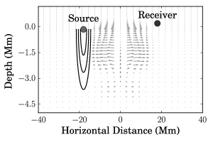
Figure 1: Schematic depiction of the measurement process used in our analysis. Seismic waves are emitted by the source and travel through the supergranule. The wave displacement and velocity are measured at various points on the surface referred to as “receivers”. We use eight different sources spread out horizontally to adequately sample the supergranule flow profile.

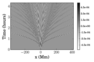
Figure 2: Vertical velocity of a wave emitted by a source at $x=0$ Mm as measured at the surface. Receivers at each horizontal location record the arrivals of seismic waves. Wavepackets reach receivers in discrete bunches, corresponding to total internal reflection at different depths.

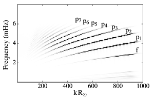
Figure 3: Spectrum of wave displacement as measured on the surface. The ridges represent radial orders that probe different depths inside the Sun. We use ridges f through $p_{7}$ in our analysis.

Seismic waves traveling through the background medium are advected by the flow field $\mathbf{v}\left(\mathbf{x}\right)$ in addition to experiencing restoring forces by pressure perturbations and gravity. The linearized wave equation for the small-amplitude displacement $\bm{\xi}\left(\mathbf{x},t\right)$ is given by

$$\rho\partial_{t}^{2}\bm{\xi}+2\rho\mathbf{v}\cdot\bm{\nabla}\partial_{t}\bm{\xi} = \bm{\nabla}\left(c^{2}\rho\bm{\nabla}\cdot\bm{\xi}+\bm{\xi}\cdot\bm{\nabla}p\right)$$ (10)

$$+\mathbf{g}\bm{\nabla}\cdot\left(\rho\bm{\xi}\right)+\mathbf{S},$$

where $\mathbf{S}=\mathbf{S}\left(\mathbf{x},t\right)$ represents sources that are exciting waves. We choose eight sources that are isolated and fire independently of each other. The fundamental measurement that we consider is the vertical velocity field of waves measured at the surface. Each spatial point at which a measurement is made is termed a “receiver”. Observations of seismic waves on the solar surface would measure source-receiver travel-times in the presence of supergranules. An incomplete model of the supergranule flow profile would produce travel-times that differ from the observed ones. The idea of full-waveform inversion, as prescribed by Hanasoge & Tromp (2014) in this context, is to iteratively reduce the misfit between the observed and predicted travel-times by altering the flow velocity in the model at each step. Denoting the travel-time measured at receiver location $\mathbf{x}_{i}$ in the model with the reference supergranule by $\tau_{i}^{o}$, and that measured in the iterated model by $\tau_{i}$, we define a least-square misfit functional

$$\chi=\frac{1}{2}\sum_{\mathbf{x}_{i}}\left(\tau_{i}-\tau_{i}^{o}\right)^{2}.$$ (11)

It should be noted that $\tau_{i}$ depends on the model flow through a complicated, as yet unknown relation $\tau_{i}\left(\mathbf{v}\left(\mathbf{x}\right)\right)$, and similarly $\tau_{i}^{o}$ depends on the reference supergranule velocity $\mathbf{v}^{\mathrm{ref}}\left(\mathbf{x}\right)$. Requiring the misfit $\chi$ to decrease at each step leads to a scheme for updating $\mathbf{v}\left(\mathbf{x}\right)$. A fundamental question still lingers — is reducing the travel-time misfit equivalent to converging to the correct supergranular flow? To investigate this, we define model misfit $\chi_{m}$ as the normalized $L_{2}$ norm of the difference between the true model $m^{\mathrm{ref}}$ and iterated model $m$,

$$\chi_{m}=\frac{\int_{B}d\mathbf{x}\left|m^{\mathrm{ref}}\left(\mathbf{x}\right)-m\left(\mathbf{x}\right)\right|^{2}}{\int_{B}d\mathbf{x}\left|m^{\mathrm{ref}}\left(\mathbf{x}\right)\right|^{2}},$$ (12)

where $B$ denotes the computational box, and the model $m$ represents the variable we are interested in, for example the vector potential $\psi$, or the individual components of the velocity $\mathbf{v}$. Another related diagnostic measure is the model misfit as a function of depth, defined as

$$\chi_{m,z}\left(z\right)=\frac{\int_{-L/2}^{L/2}dx\left|m^{\mathrm{ref}}\left(\mathbf{x}\right)-m\left(\mathbf{x}\right)\right|^{2}}{\int_{-L/2}^{L/2}dx\left|m^{\mathrm{ref}}\left(\mathbf{x}\right)\right|^{2}},$$ (13)

where $L$ is the horizontal extent of the computational box. This profile of model misfit allows us to probe the accuracy of the reconstructed flow profile as a function of depth, something that can be analyzed for each radial mode.

3 Numerics

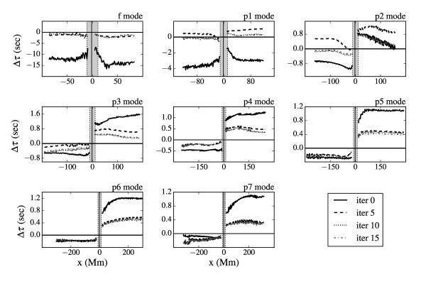
Figure 4: Travel-time difference between true and iterated models, measured at each receiver for one particular source located at $x=-2$ Mm (solid vertical line). The vertical patch centered about $x=0$ Mm represents the location of the reference supergranule. Waves being sped-up would record a negative travel-time shift whereas waves that are being slowed down would produce a positive shift. The first few iterations are dominated by the $f$ and $p_{1}$ modes, while the higher $p$ modes contribute later on, although to a limited extent.

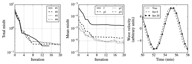
Figure 5: Left: data misfit $\chi$ (Equation (11)) — the variable that is minimized at each step — for each strategy (See Table 1). We find that data misfit falls fastest and the most in Strategy $\#1$, where we use $f$ and $p_{1}$ modes. Middle: average modal travel-time misfit per source-receiver pair for strategy $\#3$, where we use modes $f$ through $p_{7}$. Only the four lowest radial orders are plotted. Right: A section of $f$-mode waveforms at the start and after $35$ iterations for strategy $\#3$, for a source at $x=-2$ Mm and a receiver at $x=18$ Mm.

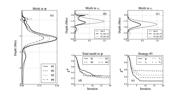
Figure 6: Model misfits in the various strategies. (a) Horizontally integrated misfit in vector potential $\psi$ as a function of depth (Equation (13) with $m=\psi$) for strategies $\#1$ through $\#4$; (b) horizontally integrated misfit in the horizontal component of velocity $v_{x}$ as a function of depth; (c) horizontally integrated misfit in the vertical component of velocity $v_{z}$ as a function of depth; (d) total model misfit for $\psi$ (Equation (12) with $m=\psi$) as a function of iterations for strategies $\#1$ through $\#4$; (e) model misfit for vector potential (solid line), vertical velocity component $v_{z}$ (dot-dashed line), horizontal velocity component $v_{x}$ (dashed line), $v_{x}$ considering only the sub-surface layers (dots, denoted by $\tilde{v}_{x}$ in the legend) with iteration for Strategy $\#3$, that uses modes $f$ through $p_{7}$.

Figure 7: The leftmost panels represent the horizontal component of flow (top) and the vertical component (bottom) of the reference supergranule. Panels second from left onwards show the iterated velocity profile corresponding to strategies $\#1$ through $\#4$. The horizontal dotted line indicates the surface ($z=0$ Mm).

We use the wave propagation code SPARC (Hanasoge, 2007) to carry out simulations and measure source-receiver travel-times. SPARC uses a second-order, five-stage low dissipation and dispersion Runge-Kutta time-evolution scheme (Hu et al., 1996), where spatial derivatives are computed using spectral (horizontal) and sixth-order compact finite-difference (vertical; Lele, 1992) schemes. We choose a grid that spans $800$ Mm horizontally resolved using $512$ points, and vertically extends from $137$ Mm below the photosphere to $1.18$ Mm above it over $300$ points. The computational grid is assumed to be periodic in the horizontal direction. The vertical grid points are equally spaced in acoustic radius, with perfectly-matched absorbing layers lining the upper and lower boundaries of the grid to minimize reflections back into the box.

Lacking a specific choice for the sub-surface profile of the supergranule, we start from a model that does not have any flows and iteratively update it. Flow velocity is related to the vector potential through

$$\mathbf{v}=\frac{1}{\rho}\bm{\nabla}\times\left[\rho c\left(\psi-\psi_{0}\right)\mathbf{e}_{y}\right],$$ (14)

where $\psi_{0}$ is a constant and represents the value of $\psi$ far away from the cell center, therefore choosing $\psi=\psi_{0}$ at the first step ensures that we do not have flows in our model. At each step of the iteration, we perform eight simulations with sources placed at different horizontal locations, all at a depth of $150$ km below the photosphere. We choose the horizontal coordinate of the sources lying around the center of the box so that the waves traverse a large distance through the supergranule, therefore contributing significantly to the travel-time misfit. We carry out measurements of the wave velocity at various horizontal locations at a height of $200$ km above the photosphere; the horizontal range of receiver pixels is limited by the distance traveled by the wave in the time duration of the simulation. One particular arrangement of a source and receiver position with respect to the reference supergranular flow is depicted in Figure 1.

Waves emanating from a source reaches different receivers at different times, and keeping track of the arrival at each receiver, we can construct a time-distance diagram that encodes all information about wave travel-times as measured on the surface. An example of such a time-distance diagram is given in Figure 2, where separate arrivals show up as distinct ridges. We carry out spatial and temporal Fourier transforms of the time-distance diagram to obtain the spectrum of seismic oscillations measured at the surface. One such spectrum is shown in Figure 3, where several ridges corresponding to standing modes have been marked. Waves corresponding to each mode travel at a specific phase velocity; we apply ridge-filters to isolate them and measure travel times for each ridge. We choose several different combinations of spectral ridges as listed in Table 1 to carry out the inversion and compare the eventual inferences. We apply the adjoint method — described by Hanasoge et al. (2011) in the context of helioseismology — to construct the requisite sensitivity kernel to update our models of the vector potential. We describe these kernels in the appendix. The kernel represents the gradient of the misfit functional $\chi$ with respect to the vector potential $\psi$; we precondition the kernel using an “approximate Hessian” (Fichtner & Trampert, 2011; Zhu et al., 2013). We smooth the kernels horizontally and vertically to remove high-spatial-frequency variations, this acts as a regularization by moderating the absolute values of high order derivatives. We apply a Gaussian smoothing: we use a spectral smoothing horizontally with a standard deviation of $4$ wavenumbers, and a spatial smoothing vertically with widths as listed in Table 1. These kernels are used to update our model using the Polak–Ribière variant of the non-linear conjugate gradient scheme (Nocedal & Wright, 2006).

Strategy	Modes	Vertical Smoothing
$\#1$	$f$ and $p_{1}$	$2$ pixel
$\#2$	$f$, $p_{1}$ to $p_{3}$	$2$ pixel
$\#3$	$f$, $p_{1}$ to $p_{7}$	$2$ pixel
$\#4$	$f$, $p_{1}$ to $p_{7}$	$8$ pixel

Table 1: Strategies used to generate and regularize sensitivity kernels used in the inversion.

Waves corresponding to different modes contribute differently to the travel-time misfit. We show the variation of travel-time misfit as measured at each receiver in Figure 4. We compare the reduction in data misfit for the different strategies in Figure 5. We find that the data misfit corresponding to each radial order falls by about an order of magnitude. The corresponding waveforms are well matched and further iterations do not improve the misfit significantly. A question that we seek to address is — to what extent does a decrease in data misfit translate to an improvement in the supergranule flow profile? We compare the improvement in model misfit for each strategy in Figure 6. We find that strategy $1$ is able to capture many essential structural features of the flow profile, including the return flow, whereas incorporating higher order $p$-modes modes leads to updates concentrated at the surface and above it. We plot the iterated velocity profiles corresponding to the different strategies in Figure 7. We observe that the iterations try to reach a compromise between the flow profile above and below the surface. As a result, including higher order $p$-modes does not lead to a significant improvement in the profile. The misfit reduces somewhat in strategy $\#4$ — where we increase the degree of smoothing — since this limits the weight of the kernel towards deeper layers; however, better strategies that constrain updates to sub-surface layers need to be explored. We reach the following conclusions: (a) the deep return flow present in the reference supergranule is not correctly reconstructed in the iterations, indicating limited sensitivity at greater depths, (b) the peak magnitude of the flow components are underestimated by the inversion process, (c) the depth corresponding to maximum flow velocity is underestimated (d) the flow velocity the surface is overestimated. There is improvement beyond the results by Dombroski et al. (2013) in the sense that the vertical component of the flow resembles the reference model, at least qualitatively, however the magnitudes of the velocities are mismatched.

A similar analysis can be carried out for sound-speed perturbations, and has been presented in the Appendix. This serves as a contrast to the inversion for supergranular flow, and lets us compare the rates of convergence in the two cases for the same strategies. We find that the inversion for sound-speed perturbation converges faster and more accurately than that of the supergranular flow, but estimates a shallower and weaker perturbation similar to that for the flow. This seems to hint at a shortcoming of the inversion process.

4 Discussion

Estimating small-scale sub-surface flows in the Sun is a fundamental challenge of local helioseismology. Supergranular flows have proven hard to image accurately, and despite considerable efforts, a consensus regarding the optimal strategy has remained elusive. In this work, we tested the effectiveness of full-waveform inversion in the context of sub-surface supergranular flows. We generated synthetic data by simulating seismic waves in presence of an axisymmetric supergranule. We used travel-times of seismic waves measured on the surface to define a misfit functional that encodes the difference between the reference supergranule and a test model of the flow profile. We applied the adjoint method (Hanasoge et al., 2011) to construct kernels and iteratively improved our model using the nonlinear conjugate-gradient algorithm to reduce the travel-time misfit. We compared several inversion strategies by varying the number of eigenmodes involved in the inversion as well as the level of regularization. We found that

• including high order $p$-modes focuses the inversion on surface layers at the expense of sub-surface layers. A similar near-surface deviation was found even for a sound-speed perturbation. The inferences might improve by imposing a surface constraint on the quantity being inverted for.

• the reconstructed vector potential has smoother gradients than the true model and hence the magnitudes of velocity are underestimated.

One possible factor that is keeping the iterations from converging onto the true model is the high dimension of the model space. In this work we have sought kernels defined on a grid of $1.5\times 10^{5}$ points. Smoothing reduces the number of independent parameters, but the inversion is not well constrained — the updates are not localized to the spatial extent of the reference supergranule. A better approach might be to expand the supergranule in an appropriate basis, an approach similar to global seismic inversions for solar rotation. This might lead to better convergence, and will be explored in future work. One extra simplification that we carried out in this analysis was that we used two-dimensional simulations to construct kernels, leaving out scatterings off the $x-z$ plane. All such scatterings carry different information about the flow profile — even if the reference model that we are trying to invert for is axisymmetric — and therefore might improve the convergence.

In this work we have not split waves into frequency regimes to study their sensitivities to the flow. A frequency filtered approach to inversion is common in terrestrial seismology, where lower frequencies are introduced first and higher ones gradually during the iterative inversion, with the order being important. Lower frequencies for a specific radial order probe deeper layers than higher frequencies, therefore such an approach might be useful infer these layers first; however, the range of frequencies in helioseismology is limited to a a factor of $3$, whereas the frequency range spans orders of magnitude in geophysics. Notwithstanding this, an approach that separates out spatial and frequency scales is worth pursuing to obtain better inferences.

Our analysis assumes that there is no noise in the measured wave velocity, and therefore the travel-times measurements are precise, but this is far from what is expected in reality. Hanasoge et al. (2011) prescribed a strategy to construct a misfit functional that includes a noise covariance matrix; a similar full-waveform inversion analysis with such a definition of misfit would represent what we might expect in solar observations.

JB would like to acknowledge the financial support provided by Department of Atomic Energy, India.

Appendix A Kernels and Updates

We study the source-receiver travel-time for waves belonging to different modes, ranging from $f$ through $p_{7}$. Waves corresponding to each mode sense different regions in the solar interior, and hence contributes differently to the inversion. The response of waves to a small change in the model of sub-surface flows is represented by $\mathbf{K_{v}\left(\mathbf{x}\right)}=\left(K_{v_{x}}\left(\mathbf{x}\right),K_{v_{z}}\left(\mathbf{x}\right)\right)$, where the components describe the sensitivity of seismic waves to horizontal and vertical components of flow velocity respectively. The functional representation of $\mathbf{K_{v}\left(\mathbf{x}\right)}$ in terms of the wave-field can be obtained by using the adjoint method; the procedure has been described by Hanasoge et al. (2011). The kernel for flow velocity can be manipulated to obtain the analogous kernel corresponding to the vector potential $\psi$ , denoted by $K_{\psi}$ (Hanasoge, 2014). The two kernels are related through

$$K_{\psi}=\rho c\psi\mathbf{e}_{y}\cdot\bm{\nabla}\times\frac{\mathbf{K_{v}}}{\rho}.$$ (A1)

We have plotted vector-potential kernels corresponding to several modes in Figure 8. The high $p$-mode kernels have sharp peaks at the surface, but are sensitive to deeper layers inside the Sun. The key to an inversion using high $p$-modes therefore seems to be to fix surface layers first — possible by starting with $f$ and $p_{1}$ modes — so that the depth-sensitivity of these modes is not masked by near-surface corrections. The strategy seems contradictory to the geophysics technique of introducing low frequencies first, so a conclusion has to be deferred.

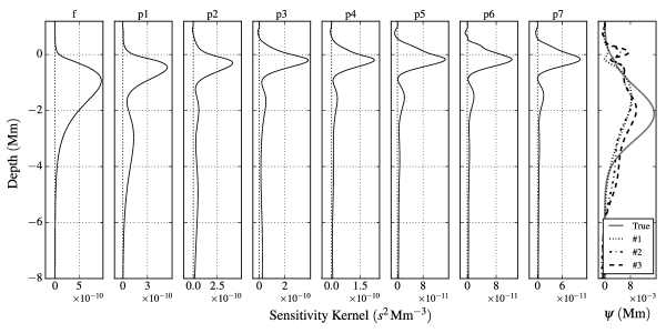
Figure 8: Horizontally integrated sensitivity kernels corresponding to modes of different radial orders, for the vector potential $\psi$ (eight panels from the left). Rightmost panel: True and inverted vector potentials contrasted.

We validated the flow kernels for single source-receiver travel-times by comparing two models: one being that of a quiet sun, the other model included a spatially constant flow $\delta v_{x}=1\,\mathrm{m/s}$. For a single source at point $\mathbf{x}_{s}$ and receiver at point $\mathbf{x}_{r}$, the travel-time misfit can be expressed as

$$\chi=\frac{1}{2}\left(\tau_{r}-\tau_{r}^{o}\right)^{2},$$ (A2)

and a small change in model would shift this misfit by

$$\delta\chi=\left(\tau_{r}-\tau_{r}^{o}\right)\delta\tau_{r}.$$ (A3)

We can express this in terms of the sensitivity kernel for the flow as

$$\delta\chi = \left(\tau_{r}-\tau_{r}^{o}\right)\frac{\partial\tau_{r}}{\partial\mathbf{v}}\delta\mathbf{v}$$ (A4)

$$= \int d\mathbf{x}\,\mathbf{K_{v}}\left(\mathbf{x}\right)\cdot\delta\mathbf{v}.$$

We can measure $\delta\chi$ by comparing the waveforms arriving at the receiver point $\mathbf{x}_{i}$ in the two models. We verified that the equality in Equation (A4) was maintained for a range of distances, thereby validating the kernels.

Once we have the kernels, we update our model as follows (Nocedal & Wright, 2006; Fichtner & Trampert, 2011):

Given $x_{0}$, evaluate $f_{0}=f\left(x_{0}\right),\;\bm{\nabla}f_{0}=\bm{\nabla}f\left(x_{0}\right)$. Set $p_{0}\leftarrow-\bm{\nabla}f_{0},\;k\leftarrow 0$.

while $\bm{\nabla}f_{k}\neq 0$

Evaluate $\alpha_{k}$ using a line-search

Evaluate $x_{k+1}=x_{k}+\alpha p_{k}$; $\bm{\nabla}f_{k+1}=\bm{\nabla}f\left(x_{k+1}\right)$

Precondition using “approximate Hessian” $\bm{\nabla}f_{k+1}\leftarrow H\bm{\nabla}f_{k+1}$

Compute the following:

$$\beta_{k+1} \leftarrow \frac{\bm{\nabla}f_{k+1}^{T}\left(\bm{\nabla}f_{k+1}^{T}-\bm{\nabla}f_{k}^{T}\right)}{\left\|\bm{\nabla}f_{k}\right\|^{2}},$$

$$p_{k+1} \leftarrow -\bm{\nabla}f_{k+1}+\beta_{k+1}p_{k},$$

$$k \leftarrow k+1,$$

end while.

Appendix B Sound-speed perturbation

We carry out an analysis similar to the supergranule flow profile by starting with a specific perturbation to the sound-speed profile, with a functional form given by

$$\delta\ln c=\exp\left(-\frac{x^{2}}{2\sigma_{x}^{2}\left(z\right)}-\frac{\left(z-z_{0}\right)^{2}}{2\sigma_{z}^{2}}\right),$$ (B1)

where $z_{0}=-2.5$ Mm, $\sigma_{z}=1.4$ Mm, and

$$\sigma_{x}\left(z\right)=10\,\mathrm{Mm}\left(1+\exp\left(\frac{z}{10\,\mathrm{Mm}}\right)\right).$$ (B2)

We use modes $p_{1}$ to $p_{7}$ to carry out the inversion, leaving out the $f$ mode since it is not significantly affected by a sound-speed perturbation. The data and model misfits after $35$ iterations have been plotted in Figure 9. We find that the model misfit falls to $0.06$, corresponding to a decrease in data misfit by a factor of around $10^{3}$. True and iterated sound-speed perturbations are plotted in Figure 10. The important conclusions that arise from this analysis are: (a) the data misfit for this sound-speed perturbation falls by three orders of magnitude, as opposed to one order for supergranular flows, (b) the inversion converged faster for this sound-speed perturbation than that for the supergranular flow.

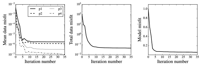
Figure 9: Data misfit for the sound-speed perturbation described in Equation B1. Left: Mean data misfit per source-receiver pair for four of the seven radial mode used in the inversion. Center: Total data misfit summed over all sources, receivers and modes ($\chi$ as in equation (11)). Right: model misfit ($\chi_{m}$ as in Equation (12), with $m=\delta\ln c$). We find that the inversion converges by iteration $10$, further iterations leading to tiny improvements to the model.

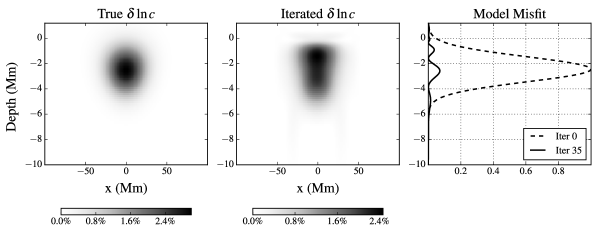
Figure 10: Left: True sound-speed perturbation. Center: Inverted sound-speed perturbation after $35$ iterations. Right: horizontally integrated model misfit ($\chi_{m,z}$ as in Equation (13), with $m=\delta\ln c$).

References

- Christensen-Dalsgaard et al. (1996) Christensen-Dalsgaard, J., Dappen, W., Ajukov, S. V., et al. 1996, Science, 272, 1286
- DeGrave & Jackiewicz (2015) DeGrave, K., & Jackiewicz, J. 2015, Sol. Phys., 290, 1547
- Dombroski et al. (2013) Dombroski, D. E., Birch, A. C., Braun, D. C., & Hanasoge, S. M. 2013, Sol. Phys., 282, 361
- Duvall & Hanasoge (2013) Duvall, T. L., & Hanasoge, S. M. 2013, Sol. Phys., 287, 71
- Duvall & Birch (2010) Duvall, Jr., T. L., & Birch, A. C. 2010, ApJ, 725, L47
- Duvall et al. (1993) Duvall, Jr., T. L., Jefferies, S. M., Harvey, J. W., & Pomerantz, M. A. 1993, Nature, 362, 430
- Duvall et al. (1997) Duvall, Jr., T. L., Kosovichev, A. G., Scherrer, P. H., et al. 1997, Sol. Phys., 170, 63
- Fichtner & Trampert (2011) Fichtner, A., & Trampert, J. 2011, Geophysical Journal International, 185, 775
- Gizon & Birch (2002) Gizon, L., & Birch, A. C. 2002, ApJ, 571, 966
- Hanasoge et al. (2012) Hanasoge, S., Birch, A., Gizon, L., & Tromp, J. 2012, Physical Review Letters, 109, 101101
- Hanasoge (2007) Hanasoge, S. M. 2007, PhD thesis, Stanford University
- Hanasoge (2014) —. 2014, ApJ, 797, 23
- Hanasoge et al. (2011) Hanasoge, S. M., Birch, A., Gizon, L., & Tromp, J. 2011, ApJ, 738, 100
- Hanasoge et al. (2007) Hanasoge, S. M., Duvall, Jr., T. L., & Couvidat, S. 2007, ApJ, 664, 1234
- Hanasoge & Tromp (2014) Hanasoge, S. M., & Tromp, J. 2014, ApJ, 784, 69
- Hathaway et al. (2000) Hathaway, D. H., Beck, J. G., Bogart, R. S., et al. 2000, Sol. Phys., 193, 299
- Hu et al. (1996) Hu, F. Q., Hussaini, M. Y., & Manthey, J. L. 1996, Journal of Computational Physics, 124, 177
- Jackiewicz et al. (2007) Jackiewicz, J., Gizon, L., Birch, A. C., & Duvall, Jr., T. L. 2007, ApJ, 671, 1051
- Kosovichev et al. (2000) Kosovichev, A. G., Duvall, Jr., T. L. ., & Scherrer, P. H. 2000, Sol. Phys., 192, 159
- Lele (1992) Lele, S. K. 1992, Journal of Computational Physics, 103, 16
- Nocedal & Wright (2006) Nocedal, J., & Wright, S. J. 2006, Numerical Optimization, 2nd edn. (New York: Springer)
- Rieutord et al. (2008) Rieutord, M., Meunier, N., Roudier, T., et al. 2008, A&A, 479, L17
- Švanda et al. (2011) Švanda, M., Gizon, L., Hanasoge, S. M., & Ustyugov, S. D. 2011, A&A, 530, A148
- Zhu et al. (2013) Zhu, H., Bozdağ, E., Duffy, T. S., & Tromp, J. 2013, Earth and Planetary Science Letters, 381, 1