The Distribution of Mass Surface Densities in a High-Mass Protocluster

Abstract

We study the probability distribution function (PDF) of mass surface densities, $\Sigma$, of infrared dark cloud (IRDC) G028.37+00.07 and its surrounding giant molecular cloud. This PDF constrains the physical processes, such as turbulence, magnetic fields and self-gravity, that are expected to be controlling cloud structure and star formation activity. The chosen IRDC is of particular interest since it has almost 100,000 solar masses within a radius of 8 parsecs, making it one of the most massive, dense molecular structures known and is thus a potential site for the formation of a “super star cluster.” We study $\Sigma$ in two ways. First, we use a combination of NIR and MIR extinction maps that are able to probe the bulk of the cloud structure up to $\Sigma\sim 1\>{\rm{g\>cm}^{-2}}\>$($A_{V}\simeq 200$ mag). Second, we study the FIR and sub-mm dust continuum emission from the cloud utilizing Herschel PACS and SPIRE images and paying careful attention to the effects of foreground and background contamination. We find that the PDFs from both methods, applied over a $\sim 20^{\prime}$(30 pc)-sized region that contains $\simeq 1.5\times 10^{5}\>M_{\odot}$ and encloses a minimum closed contour with $\Sigma\simeq 0.013\>{\rm{g\>cm}^{-2}}\>$($A_{V}\simeq 3$ mag), shows a log-normal shape with the peak measured at $\Sigma\simeq 0.021\>{\rm{g\>cm}^{-2}}\>$($A_{V}\simeq 4.7$ mag). There is tentative evidence for the presence of a high-$\Sigma$ power law tail that contains from $\sim 3\%$ to 8% of the mass of the cloud material. We discuss the implications of these results for the physical processes occurring in this cloud.

1. Introduction

The probability distribution function (PDF) of mass surface density, $\Sigma$, is one of the simplest metrics of interstellar cloud structure. This $\Sigma$-PDF is, in principle, much easier to observe than other distributions, such as volume density, thus making it a convenient metric with which to compare observed and simulated clouds. The $\Sigma$-PDF shape should be sensitive to physical processes occurring in the clouds. For example, simulations of driven supersonic hydrodynamic (and if including magnetic fields, super-Alfvénic) turbulence of non-self-gravitating gas in periodic boxes yield lognormal $\Sigma$-PDFs (e.g., Federrath 2013; Padoan et al. 2014), i.e., the area-weighted PDF, $p_{A}$, can be well-fit by a lognormal:

$$p_{A}({\rm{ln}}\Sigma^{\prime})=\frac{1}{(2\pi)^{1/2}\sigma_{\rm{ln}\Sigma^{\prime}}}{\rm{exp}}\left[-\frac{({\rm{ln}}\Sigma^{\prime}-\overline{{\rm{ln}}\Sigma})^{2}}{2\sigma_{\rm{ln}\Sigma^{\prime}}^{2}}\right],$$ (1)

where $\Sigma^{\prime}\equiv\Sigma/\overline{\Sigma}_{\rm{PDF}}$ is mean-normalized $\Sigma$. The lognormal width, $\sigma_{\rm{ln}\Sigma}$, grows as turbulent Mach number increases. In simulations with self-gravity, $\Sigma$-PDFs are seen to develop high-end power law tails, perhaps tracing regions undergoing free-fall collapse (Kritsuk et al. 2011; Collins et al. 2011; Cho & Kim 2011; Federrath & Klessen 2013). However, simulations of self-gravitating, strongly-magnetized (trans-Alfvénic), turbulent clouds with non-periodic boundary conditions are also needed for comparison with observed $\Sigma$-PDFs. Such clouds are expected to have smaller star formation efficiencies per mean free-fall time, $\epsilon_{\rm{ff}}$, likely implying they would have smaller mass fractions in any high-$\Sigma$ power law tail. Accurate quantification of the $\Sigma$-PDF in real star-forming clouds is needed to constrain theoretical models.

Observationally, Kainulainen et al. (2009 [K09]) performed NIR extinction mapping of $\sim$20 nearby clouds, ranging from “quiescent,” non-star-forming clouds to more active clouds. They found quiescent cloud $\Sigma$-PDFs are well-described by lognormals, while star-forming clouds have high-$\Sigma$ power law tails. Note, in practice a lognormal is fit to the observed $p_{A}({\rm{ln}}\Sigma)$, which is then used to derive $\overline{\rm{ln}\Sigma}$ (over the considered range of $\Sigma$), which then defines the mean $\overline{\Sigma}_{\rm{PDF}}\equiv{e}^{\overline{\rm{ln}\Sigma}+\sigma^{2}_{\rm{ln}\Sigma}/2}$, where $\sigma_{\rm{ln}\Sigma}$ is standard deviation of $\rm{ln}\Sigma$ (Butler et al. 2014, hereafter BTK14).

However, the ability of this observational method to accurately measure the position of the $\Sigma$-PDF peak, typically at $\Sigma\sim 0.01\>{\rm{g\>cm}^{-2}}$ (i.e., $A_{V}\sim 2\>{\rm{mag}}$: we adopt conversion $\Sigma/(1\>{\rm{g\>cm}^{-2}})\equiv{A}_{v}/(224.8\>{\rm{mag}})$ (Kainulainen & Tan 2013 [KT13]) in the K09 clouds, has been questioned by Schneider et al. (2015a) and Lombardi et al. (2015) due to difficulties of disentangling foreground and background contributions. Lombardi et al. argued that low-$\Sigma$ PDF uncertainties are so large that observed PDFs are all consistent with power laws.

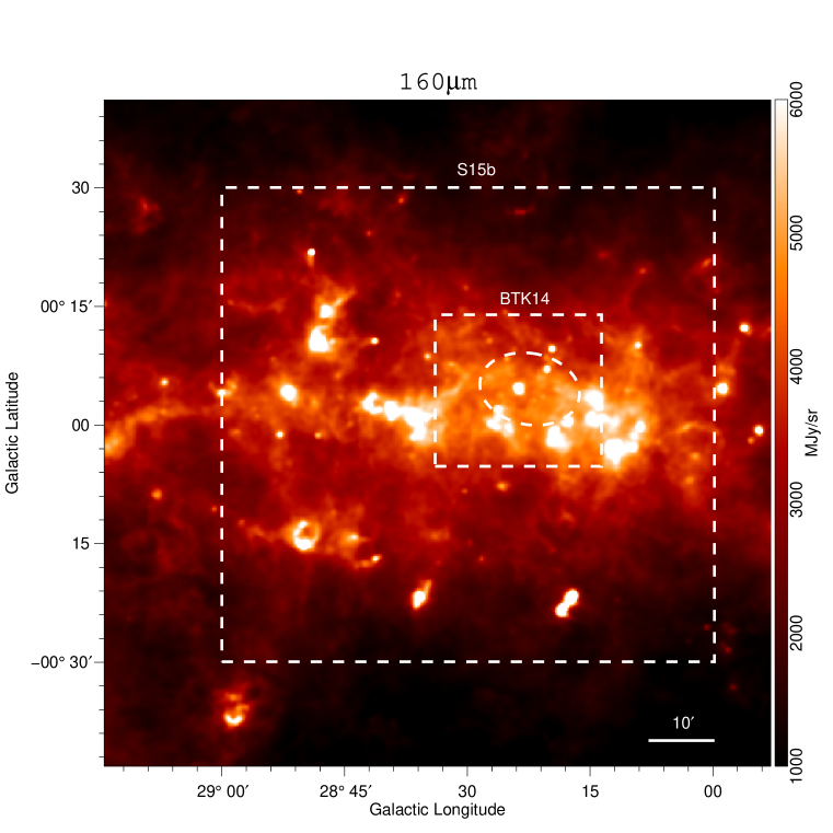
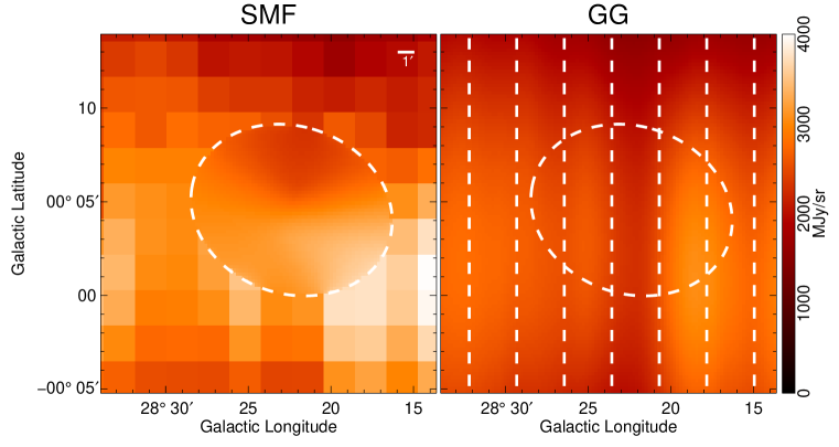
Figure 1.— (a) Top: $160\>{\rm{\mu}{m}}$ image of IRDC G028.37+00.07 (ellipse) and surroundings. Smaller rectangle shows $20\arcmin\times 19\arcmin$ area analyzed by BTK14 and in this Letter. Larger rectangle indicates approximate area, $\sim 1\arcdeg\times 0.7\arcdeg$, studied by S15b. (b) Bottom Left: Galactic background model for $160\>{\rm{\mu}{m}}$ intensity for the BTK14 region evaluated with Small Median Filter (SMF) method. (c) Bottom Right: As (b), but with Galactic Gaussian (GG) method. The seven vertical lines are locations of profiles shown in Fig. 2.

Extending these studies to denser, higher-$\Sigma$ clouds, perhaps more typical of most Galactic star formation, KT13 used combined NIR (Kainulainen et al. 2011) + MIR (Butler & Tan 2012 [BT12]) extinction maps to study $\Sigma$-PDFs of 10 IRDCs. These dense structures, typically several kpc away, have $\Sigma$-PDFs extending to $\sim 1\>{\rm{g\>cm}^{-2}}$ (e.g., Tan et al. 2014). One uncertainty of these maps is choice of opacity (i.e., at $8\>{\rm{\mu}{m}}$) per unit $\Sigma$, with variations $\sim 30\%$ expected for different dust models, e.g., moderately coagulated thin and thick ice mantle models of Ossenkopf & Henning (1994 [OH94]). KT13 considered simple, rectangular regions enclosing contours of $\Sigma=0.03\>{\rm{g\>cm}^{-2}}$ ($A_{V}\simeq 7\>$mag), i.e., “complete” for $\Sigma$ above this value. However, two caveats limit this completeness: first, MIR-bright regions are not treated by extinction mapping, so are excluded from the PDF; second, extinction mapping saturates at high-$\Sigma$’s, depending on MIR image depth, typically at $\sim 0.3\>$to$\>0.5\>{\rm{g\>cm}^{-2}}$ for Spitzer GLIMPSE (Churchwell et al. 2009) images (BT12). At low-$\Sigma$’s, better probed by NIR extinction mapping, systematic uncertainties are $\sim 0.01\>{\rm{g\>cm}^{-2}}$. The KT13 $\Sigma$-PDFs, extending down to $A_{V}=7\>$mag, did not cover PDF peaks well, so provided weak constraints on true shapes: PDFs could be fit with lognormals or power laws.

BTK14 presented a higher dynamic range $\Sigma$-map of IRDC G028.37+00.07, both to higher $\Sigma\simeq 0.7\>{\rm{g\>cm}^{-2}}$ and lower $\Sigma\simeq 0.013\>{\rm{g\>cm}^{-2}}$ ($A_{V}\simeq 3\>$mag). From a $20\arcmin\times 19\arcmin$ region around the IRDC (Fig. 1a), BTK14 derived a $\Sigma$-PDF where the peak was observed at $\Sigma_{\rm{peak}}\simeq 0.03\>{\rm{g\>cm}^{-2}}$. Furthermore, the entire PDF from $0.013\>$to$\>0.4\>{\rm{g\>cm}^{-2}}$ was well-described by a lognormal with $\overline{\Sigma}_{\rm{PDF}}=0.039\>{\rm{g\>cm}}^{-2}$ ($\overline{A}_{V,{\rm{PDF}}}=9.0\>$mag) and $\sigma_{\rm{ln}\Sigma^{\prime}}=1.4$. There appears to be relatively little mass in a high-$\Sigma$ power law tail, surprising given the IRDC (KT13) and GMC (Hernandez & Tan 2015 [HT15]) are both self-gravitating with virial parameters close to unity and some star formation has already started.

Another method to measure $\Sigma$ is via sub-mm dust continuum emission. However, this also depends on dust temperature, $T$, so multiwavelength studies are needed to probe the spectral energy distribution (SED) peak. The best data for this comes from Herschel PACS and SPIRE observations probing $70\>$to$\>500\>{\rm{\mu}{m}}$. However, derived maps have angular resolution $\sim 20\arcsec$, i.e., $\sim 10\times$ worse than the NIR+MIR extinction maps.

Schneider et al. (2015b [S15b]) utilized Herschel-derived $\Sigma$-maps to study the same IRDC/GMC examined by BTK14. They derived $\Sigma$-PDFs for the IRDC ellipse region (Fig. 1a) and a surrounding “GMC” region defined by a ¹³CO(1-0) emission contour equivalent to $A_{V}\sim 2\>$mag, extending approximately over the larger rectangle shown in Fig. 1. Note, this is significantly larger than the BTK14 region. S15b found their IRDC $\Sigma$-PDF was well-fit by a single power-law for $A_{V}\gtrsim 30\>$mag. The GMC region could also be fit with a power law, especially for $A_{V}\gtrsim 40\>$mag. Below this S15b claimed to detect a peak in the $\Sigma$-PDF at $A_{V}\sim 20\>$mag. S15b proposed that presence of power law tails indicated the cloud was undergoing multi-scale, including global, quasi-free-fall collapse.

Here we revisit the $\Sigma$-PDF toward IRDC/GMC G028.37+00.07, especially comparing PDFs derived from dust extinction and emission methods. We examine reasons for the different results of BTK14 and S15b and derive the most accurate $\Sigma$-PDF of this massive protocluster.

2. Methods

2.1. NIR+MIR Extinction Derived $\Sigma$ Map

We utilize the NIR+MIR extinction map from BTK14 with one modification. The NIR extinction map, based on statistical estimates of stellar extinctions in $\sim 30^{\prime}$ regions, requires choosing an “off-position” of negligible local IRDC/GMC extinction. BTK14 utilized an off-position at $l=28.4^{\circ},\>b=-0.04^{\circ}$. However, S15b noted this location may be too close to the GMC, which is confirmed in the ¹³CO(1-0) map of HT15. We therefore choose a new off-position at $l=28.3^{\circ},\>b=+0.3^{\circ}$ with $A_{V}$ that is $3\>$mag smaller than the previous position. The net effect is to add an offset of $A_{V}=3\>$mag to the BTK14 map. We will see this has only a minor effect on the $\Sigma$-PDF: in particular, the mean extinction remains close to $\overline{A}_{V,{\rm{PDF}}}\sim 9\>$mag.

Conversion of the extinction map into a $\Sigma$-map requires an assumption about opacity per unit mass at a given wavelength. Here for the Spitzer IRAC $\sim 8\>{\rm{\mu}{m}}$ map we adopt $7.5\>{\rm{cm^{2}\>g}}^{-1}$ (BT12). The NIR+MIR combination assumes $\tau_{\rm{8{\mu}{m}}}=0.29\tau_{K}$ (KT13). For conversion to $A_{V}$ we follow KT13, adopting $\Sigma/(1\>{\rm{g\>cm}^{-2}})\equiv{A}_{V}/(224.8\>{\rm{mag}})$. Overall, from consideration of different dust models (BT12), we estimate $\sim 30\%$ systematic uncertainties due to these opacity choices.

2.2. Sub-mm Emission Derived $\Sigma$ Map

$\begin{array}[]{c}\includegraphics[width=180.67499pt]{BGprofiles.eps}\\ \end{array}$

Figure 2.— Seven example profiles of the Galactic Gaussian (GG) background model (dashed lines), evaluated along $l$ values shown in Fig. 1c. Solid lines show total observed intensity (after FG subtraction), dashed lines show fitted Gaussian function to this profile, and dotted line is GG FG model. Vertical dot-dashed lines show Galactic latitude range of BTK14 region.

We use PACS and SPIRE images from the Herschel Infrared GALactic plane survey (Hi-GAL; Molinari et al. 2010). Derivation of $\Sigma$ and $T$ is performed via pixel-by-pixel graybody fits to the $160,\>250,\>350\>$and$\>500\>{\rm{\mu}{m}}$ data (e.g., Battersby et al. 2011; S15b), first re-gridded at the $500\>{\rm{\mu}{m}}$ image resolution of 36$\arcsec$. Specifically, $\Sigma$ and $T$ are derived via:

$$I_{\nu}\simeq{B}_{\nu}(1-e^{-\tau_{\nu}})=B_{\nu}(1-e^{-\Sigma\kappa_{\nu}})$$ (2)

where $I_{\nu}$ is observed intensity of the corresponding band, $B_{\nu}$ is filter-weighted value of the Planck function, $\tau_{\nu}$ is optical depth and $\kappa_{\nu}$ is filter-weighted opacity.

However, to derive local cloud properties, the images need correction for foreground (FG) and background (BG) diffuse ISM emission along the line of sight. Assuming emission from the cloud in these sub-mm bands is optically thin, one method is to estimate FG+BG emission as one combined, constant intensity. S15b adopted this method, selecting a region outside the GMC of interest for FG+BG column density corresponding to $A_{V}\simeq 2\>$mag, which was then subtracted as a constant offset.

We first assess the FG based on the ISM model derived from observed $24\>{\rm{\mu}{m}}$ intensities towards “saturated” dark regions of the IRDC by LT14 and Lim, Carey & Tan (2015 [LCT15]). These saturated regions, also seen at shorter wavelengths and possibly at $70\>{\rm{\mu}{m}}$, are where observed intensities are similar to within instrumental noise in spatially independent locations. This is assumed to be caused by the IRDC blocking essentially all BG light, so the observed intensity is that of a spatially smooth FG. Several $24\>{\rm{\mu}{m}}$ FG measurements across the IRDC are made and then averaged to estimate a mean. Then the Draine & Li (2007) diffuse ISM SED model is normalized to this value to predict $160,\>250,\>350,\>500\>{\rm{\mu}{m}}$ filter-weighted FG values. These are subtracted from the sub-mm images, i.e., the FG is first assumed to be constant across the IRDC/GMC.

Once we have FG-subtracted images, we next assess the BG in two ways. First, we assess BG intensity at each wavelength adapting the “Small Median Filter” (SMF) method (Butler & Tan 2009 [BT09]), which is applied outside the IRDC ellipse with square filter of 35$\arcmin$ size. BG emission behind the IRDC ellipse is estimated via interpolation from the surrounding regions (Fig. 1b), following the BT09 weighting scheme.

As a second, “Galactic Gaussian” (GG), method we follow Battersby et al. (2011) and assume that the Galactic BG follows Gaussian profiles in latitude. We fit Gaussians to the minimum intensities exhibited along strips with longitude width $\sim 2\arcmin$ (see Fig. 1c and Fig. 2 for examples at $160\>{\rm{\mu}{m}}$). The method involves clipping higher intensity values arising from discrete clouds, and iteratively converges on a final result. Note, here we also assume the FG intensity is a Gaussian of the same width, and subtract that off the images before deriving the final BG model.

The above methods result in FG+BG-subtracted images at $160,\>250,\>350\>\&\>500\>{\rm{\mu}{m}}$. Then at each pixel we fit the graybody function (eq. 2), including its filter response weighting, to derive $\Sigma$ and $T$. This fitting requires an assumed form of $\kappa_{\nu}$. This has been studied via MIR to FIR extinction by LT14 and LCT15, who find evidence of generally flatter extinction laws over the $\sim 8$ to $70\>{\rm{\mu}{m}}$ range as $\Sigma$ increases, consistent with OH94 and Ormel et al. (2011) dust models that include grain growth via ice mantle formation and coagulation. For consistency with these extinction results, we adopt the OH94 thin ice mantle model with $10^{5}\>$yr of coagulation at density of $n_{\rm{H}}=10^{6}\>{\rm{cm}}^{-3}$ as our fiducial. At sub-mm wavelengths, this model exhibits $\kappa_{\nu}=0.1\>(\nu/1000\>{\rm{GHz}})^{\beta}\>{\rm{cm}}^{2}\>{\rm{g}}^{-1}$ with $\beta\simeq 1.8$. We will also explore the effects of varying $\beta$ from 1.5 to 2.

Finally, we generate higher resolution (HiRes) $\Sigma$ maps by re-gridding to the $250\>{\rm{\mu}{m}}$ image pixels (18$\arcsec$ resolution; 6$\arcsec$ pixels) and then repeating the above analysis, but now fixing temperatures from the lower angular resolution maps. These HiRes $\Sigma$ maps are better able to probe smaller, higher $\Sigma$ structures.

3. Results

3.1. Mass surface density and temperature maps

$\begin{array}[]{cc}\includegraphics[width=469.75499pt]{cSmapsF3.eps}\\ \includegraphics[width=469.75499pt]{cTmapsF3.eps}\\ \includegraphics[width=469.75499pt]{cImapsIR.eps}\\ \end{array}$

Figure 3.— Sub-mm emission derived HiRes $\Sigma$ (top row) and $T$ (middle row) maps based on no FG+BG subtraction (left), SMF (middle) and GG (right) methods. Bottom row shows images from Spitzer-IRAC $8\>{\rm{\mu}{m}}$, -MIPS $24\>{\rm{\mu}{m}}$ and Herschel-PACS $70\>{\rm{\mu}{m}}$.

Figure 3 shows the sub-mm emission derived $\Sigma$ (HiRes) and $T$ maps of the IRDC, starting from maps derived with no FG and BG subtraction, and then showing the effects of the two background estimation methods (SMF and GG). The overall result of FG+BG subtraction on the $\Sigma$ map is to effectively remove $\sim 0.1\>{\rm g\>cm^{-2}}$ across the cloud. As we will see this has a major effect on the shape of the $\Sigma$-PDF. Note for study of the BTK14 region, we consider the GG method to be superior to SMF as it allows for the large-scale structure of the Galactic plane. Also, the SMF method tends to underestimate mass surface densities in the structures just outside the IRDC ellipse.

The temperature maps are also strongly affected by FG+BG subtraction, which leads to a lowering of the temperatures measured in the IRDC, as well as revealing warmer localized patches in the surroundings. Some of these appear to correspond to $8,\>24\>\&\>70\>{\rm{\mu}{m}}$-brighter regions (Fig. 3 lower panels).

The top row of Figure 4 compares the FG+BG-subtracted $\Sigma$ maps derived from NIR+MIR extinction and from sub-mm emission. White patches in the extinction map are locations of bright MIR emission that prevent an absorption measurement against the Galactic background. White patches in the sub-mm emission derived map are locations where the background subtraction has caused the estimated flux from the cloud to become negative in at least one wavelength. The second row of Fig. 4 presents the same information, but now with a simplified color scheme for the $\Sigma$ scalebar, which can be compared to regions of the $\Sigma$-PDF, discussed below.

Broadly similar morphologies are seen in these maps, but with the sub-mm emission derived maps tending to find moderately higher values in the IRDC, although the differences between the SMF and GG background subtraction methods are comparable to the differences between the Sub-mm Em. (GG) model and the extinction map. Note also the superior resolution of the extinction map.

Fig. 4’s third row shows the effect of applying different values of $\beta$ for deriving $\Sigma$ (GG case). Note $\beta=1.8$ is closest to the behavior of the OH94 thin ice mantle model. Slightly lower values of $\beta\simeq 1.5$ (which lead to warmer derived temperatures and thus lower values of $\Sigma$; e.g., Guzmán et al. 2015) are one way of reconciling differences between the extinction and emission derived maps.

Finally, Fig. 4 also shows a pixel-by-pixel comparison of $\Sigma$’s derived by NIR+MIR extinction and the fiducial sub-mm emission (GG) method. The fraction of the pixels with both $\Sigma$’s $>0.013\>{\rm{g\>cm}}^{-2}$ with values within 30% of each other is 0.608.

$\begin{array}[]{cc}\includegraphics[width=469.75499pt]{contSmaps.eps}\\ \includegraphics[width=469.75499pt]{Smapst.eps}\\ \includegraphics[width=469.75499pt]{beta1t.eps}\\ \end{array}$

Figure 4.— Top row, left-to-right: NIR+MIR extinction derived $\Sigma$ map, sub-mm emission derived $\Sigma$ map using SMF BG subtraction, sub-mm emission derived $\Sigma$ map using GG BG subtraction. Middle row, left-to-right: As top row, but with simplified color scheme for $\Sigma$ scalebar to highlight values around peak of the $\Sigma$-PDFs. Bottom row, left-to-right: Sub-mm emission derived $\Sigma$ map (GG BG subtraction), with $\beta=1.5,\>2.0$, and pixel by pixel $\Sigma$ comparison between NIR+MIR extinction and fiducial sub-mm emission (GG) methods (red lines show median and $1\sigma$ range in data binned perpendicular to the one-to-one line).

3.2. $\Sigma$ Probability Distribution Functions

$\begin{array}[]{c}\includegraphics[width=520.34377pt]{pdftestFinal.eps}\\ \includegraphics[width=520.34377pt]{pdftestFinal2.eps}\\ \end{array}$

Figure 5.— Top Row: Area-weighted $\Sigma$-PDFs of IRDC/GMC G028.37+00.07. (a) Left: Effects of foreground/background subtraction. Green solid line shows Sub-mm Em. case with no FG/BG subtracted. Green dotted line shows only FG subtracted. Brown/black solid shows SMF/GG BG subtraction, respectively. Blue solid line shows NIR+MIR extinction result, including FG+BG subtraction. (b) Middle: Effects of $\beta$ variation. Black solid line shows the fiducial Sub-mm Em. GG case, which has effective $\beta\simeq 1.8$. The $\beta=1.5,\>2$ cases are shown with dotted purple and orange lines, respectively. Variable $\beta$ model is shown with a solid purple line. (c) Right: Lognormal fits to fiducial $\Sigma$-PDFs. Shaded regions correspond to colors shown in Fig. 4 middle and bottom rows. Note grey region shows values below minimum closed contour. Bottom row, (d), (e), (f): As top row, but for mass-weighted $\Sigma$-PDFs.

Figure 5a shows the area-weighted $\Sigma$-PDF of IRDC/GMC G028.37+00.07. Note PDF normalization is with respect to the total “BTK14” area (see Fig.$\>1$). The result from the sub-mm dust emission map with no FG and BG subtracted (green solid line) is similar to S15b’s results, being intermediate between their GMC and IRDC PDFs (normalized to their particular areas), as expected given the region geometries (Fig.$\>1$). FG-only subtraction (green dotted) has a modest effect: the PDF peak moves to lower $\Sigma$ by $\simeq 0.02\>{\rm{g\>cm}}^{-2}$.

Background subtraction (SMF: brown solid; GG: black solid) leads to larger shifts of the PDF peak, reducing its value by factors of several. Overall the shapes of the two sub-mm emission derived $\Sigma$-PDFs are quite similar. The NIR+MIR derived PDF (blue solid) is also similar, especially to the PDF using GG background estimation.

Figure 5b illustrates effects of varying $\beta$ from 1.5 to 2 on the Sub-mm Em. (GG) PDF. Smaller values of $\beta$ reduce the amount of inferred high-$\Sigma$ material (thus boosting the low-$\Sigma$ distribution). Dust properties may vary systematically with $\Sigma$ due to grain growth (LCT15). Figure 5b also shows a simple “Variable-$\beta$” model where $\beta=1.8-0.3(\Sigma/[0.5\>{\rm{g\>cm}^{-2}}])$, i.e., lower $\beta$ in high-$\Sigma$ regions broadly consistent with models of grain growth (e.g., Ormel et al. 2011), applied iteratively until convergence is achieved. The resulting $\Sigma$-PDF is quite similar to the fiducial Sub-mm Em. (GG) case.

Figure 5c shows lognormal fits to the Sub-mm Em. (GG) and NIR+MIR Ext. derived PDFs, with $\Sigma_{\rm{peak}}\simeq 0.023,\>0.019\>{\rm{g\>cm}^{-2}}$ ($A_{V}\simeq 5.1,\>4.3\>$mag), respectively. Note, fitting is done only for $\Sigma\geq 0.013\>{\rm{g\>cm}^{-2}}$ ($A_{V}\simeq 3\>$mag), i.e., above the minimum closed contour in the NIR+MIR extinction map. With $\Sigma_{\rm{peak}}$ greater than $\Sigma$ of the minimum closed contour, the lognormal fitting is well-constrained by the data. Values of $\overline{\Sigma}_{\rm PDF}$ are $0.044,\>0.038\>{\rm{g\>cm}^{-2}}$, while $\sigma_{\rm{ln}\Sigma^{\prime}}=1.35,\>1.15$, respectively, compared to 1.4 reported by BTK14.

The $\Sigma$-PDFs are well-fit by single lognormals. The fraction of mass above $\Sigma=0.013\>{\rm{g\>cm}^{-2}}$ that is in excess of the lognormal fits in their high-$\Sigma$ ($>0.1\>{\rm{g\>cm}^{-2}}$) tails is $\epsilon_{\rm{pl}}\sim 0.08,\>0.03$ for Sub-mm Em. (GG) and NIR+MIR Ext. PDFs, respectively. Such small fractions may be consistent with similarly low values of $\epsilon_{\rm{ff}}$. Krumholz & Tan (2007) estimated $\epsilon_{\rm{ff}}\sim 0.02$, including results from observed IRDCs, while Da Rio et al. (2014) estimated $\epsilon_{\rm{ff}}\simeq 0.04$ in the Orion Nebula Cluster. However, detailed study of numerical simulations to link the mass fraction in these “tails,” i.e., $\epsilon_{\rm{pl}}$, with $\epsilon_{\rm{ff}}$ is still needed for trans-Alfvénic, turbulent, global clouds.

Note, these high-$\Sigma$ excess fractions in the PDFs are in fact not particularly well-described with power law tails to the lognormals. Given the small size of the excess fractions, the limited dynamic range of $\Sigma$ where they appear, and the potential systematic errors that enter at high $\Sigma$’s, we do not fit power law functions, but rather focus on $\epsilon_{\rm{pl}}$ as our metric for deviation of the PDF from a lognormal shape.

Note also, while we consider the GG method preferable to SMF, log-normal fitting results are not too sensitive to this choice: with SMF $\Sigma_{\rm{peak}}$ decreases by 25%, $\sigma_{\rm{ln}\Sigma^{\prime}}$ increases by 25%, and $\epsilon_{\rm{pl}}$ decreases by 20%.

Figures 5d-f mirror Figs. 5a-c, but now for mass-weighted PDFs. Values of $\Sigma_{\rm{peak}}$ of the lognormal fits are $0.060,\>0.051\>{\rm{g\>cm}^{-2}}$ for the Sub-mm Em. (GG) and NIR+MIR Ext. PDFs, respectively. Values of $\overline{\Sigma}_{\rm{PDF}}$ are $0.067,\>0.054\>{\rm{g\>cm}^{-2}}$, while $\sigma_{\rm{ln}\Sigma^{\prime}}\simeq 1.10,\>0.96$, respectively. These mass-weighted $\Sigma$-PDFs are also well-fit by single lognormals, with the PDF peak being significantly above the minimum closed contour level.

4. Discussion

We have measured the $\Sigma$-PDF from NIR+MIR extinction and sub-mm dust emission in a contiguous $30\>$pc-scale region centered on a dense, massive IRDC that extends to its surrounding GMC. This material is likely to eventually form a massive star cluster. The two methods give similar results, especially detecting the area-weighted $\Sigma$-PDF peak at $\simeq 0.021\>{\rm{g\>cm}^{-2}}$ and the mass-weighted $\Sigma$-PDF peak at $\simeq 0.055\>{\rm{g\>cm}^{-2}}$, both significantly higher than the minimum closed contour at $\simeq 0.013\>{\rm{g\>cm}^{-2}}$. Comparison of extinction and emission-based methods is important to assess systematic uncertainties. The consistency of these results increases our confidence in the reliability of the $\Sigma$ maps and their PDFs.

Some differences may result from dust opacity uncertainties, including potential systematic variations with density due to grain growth, which have greater influence on the sub-mm emission method. Angular resolution also leads to differences: the NIR+MIR extinction map has $\sim 2$″ resolution, while the sub-mm emission derived map has 18″ resolution, which will tend to smooth out high-$\Sigma$ peaks, thus limiting its ability to see highest-$\Sigma$ regions. NIR+MIR extinction mapping faces problems of saturation at high $\Sigma$, but this should only become important at $\Sigma\gtrsim 0.65\>{\rm{g\>cm}}^{-2}$ (BTK14): i.e., most of the range of $\Sigma$ of Fig. 5 is unaffected. NIR+MIR extinction mapping also fails in MIR-bright regions. Fig. 4 middle row and Fig. 5c show that a significant reason for difference in the amount of $\Sigma>0.4\>{\rm{g\>cm}}^{-2}$ material in the NIR+MIR extinction map compared to the Sub-mm Em. (GG) map results from the material around the central MIR-bright source in the IRDC. However, this is not enough to explain the claimed power law tail of S15b’s analysis. Rather, most of the difference of our results from S15b’s are caused by our higher estimate of the diffuse Galactic plane background subtraction level.

The $\Sigma$-PDFs are well-fit by single lognormals, even though this IRDC and GMC region is gravitationally bound with virial parameters of about unity (KT13; HT15). The $\Sigma$-PDF peak is greater than the minimum closed contour: i.e., peak position is not too sensitive to choice of map boundary. If we analyze a smaller $15\arcmin\times 15\arcmin$ region centered on the IRDC, then $\Sigma_{\rm{peak}}\simeq 0.023\>{\rm{g\>cm}^{-2}}$, $\sigma_{\rm{ln}\Sigma^{\prime}}=1.22$ and $\epsilon_{\rm{pl}}\simeq 0.07$ (averaging results from Sub-mm Em. (GG) and NIR+MIR extinction methods), similar to the results for the $20\arcmin\times 19\arcmin$ region. The position of this peak likely has physical significance, e.g., depending on properties of protocluster turbulence, magnetic fields and/or feedback, e.g., protostellar outflows, and thus constrains theoretical models of star cluster formation.

Another important result is the mass fraction in the high-$\Sigma$ power law tail (or lognormal excess), $\epsilon_{\rm{pl}}$. There is tentative evidence for a small tail being present at $\Sigma\gtrsim 0.2\>{\rm{g\>cm}}^{-2}$ and containing $\sim 3\>$to$\>8\%$ of the total mass, but subject to the systematic uncertainties discussed above. Still, we consider this to be the most accurate measurement of this high-$\Sigma$ lognormal excess mass fraction since we have measured $\Sigma$ with two independent methods, which both detect the lognormal peak. This mass fraction also constrains theoretical models, especially protocluster star formation rate and thus duration of star cluster formation. Relatively small $\epsilon_{\rm{pl}}$ may imply small $\epsilon_{\rm{ff}}$ (Krumholz & McKee 2005; Kritsuk et al. 2011; Federrath & Klessen 2012), and thus an extended duration for star cluster formation (Tan et al. 2006; Da Rio et al. 2014). Better quantification of the relation between $\epsilon_{\rm{pl}}$ and $\epsilon_{\rm{ff}}$ should be an additional goal of star cluster formation simulations.

References

- Battersby et al. (2011) Battersby, C., Bally, J., Ginsburg, A., et al. 2011, A&A, 535, 128
- Butler & Tan (2009) Butler, M. J. & Tan, J. C., 2009, ApJ, 696, 484
- Butler & Tan (2012) Butler, M. J. & Tan, J. C., 2012, ApJ, 754, 5
- Butler, Tan & Kainulainen (2014) Butler, M. J., Tan, J. C. & Kainulainen, J., 2014, ApJ, 782L, 30
- Cho & kim (2011) Cho, W. & Kim, J., 2011, MNRAS, 410, 8
- Churchwell et al. (2009) Churchwell, E., Babler, B., Meade, M., et al. 2009, PASP, 121, 213
- Collins et al. (2011) Collins, D. C., Padoan, P., Norman, M. L., & Xu, H. 2011, ApJ, 731, 59
- Da rio et al. (2014) Da Rio, N., Tan, J. C., Jaehnig, K. 2014, ApJ, 795, 55
- Draine & Li (2007) Draine, B. T. & Li, A. 2007, ApJ, 675, 810
- Federrath (2013) Federrath, C. 2013, MNRAS, 436, 1245
- Federrath & Klessen (2012) Federrath, C. & Klessen, R. S. 2012, ApJ, 761, 156
- Federrath & Klessen (2013) Federrath, C. & Klessen, R. S. 2013, ApJ, 763, 51
- Guzmán et al. (2015) Guzmán, A., Sanhueza, P., Contreras, Y., et al. 2015, ApJ, 815, 130
- Hernandez & Tan (2015) Hernandez, A. K. & Tan, J. C. 2015, ApJ, 809, 154
- Kainulainen et al. (2009) Kainulainen, J., Beuther, H., Henning, T., Plume, R. 2009, A&A, 508, 35
- Kainulainen & Tan (2013) Kainulainen, J. & Tan, J. C. 2013, A&A, 549, 53
- Kritsuk et al. (2011) Kritsuk, A. G., Norman, M. L. & Wagner, R. 2011, ApJ, 727, 20
- Krumholz & Mckee (2005) Krumholz, M. R. & McKee, C. F. 2005, ApJ, 630. 250
- Krumholz & Tan (2007) Krumholz, M. R. & Tan, J. C. 2007, ApJ, 654, 304
- Lim & Tan (2014) Lim, W. & Tan, J. C. 2014, ApJ, 780,29
- Lim, Carey & Tan (2015) Lim, W., Carey, S. J. & Tan, J. C. 2015, ApJ, 814,28
- Lombardi et al. (2015) Lombardi, M, Alves, J. & Lada, C. J. 2015, A&A, 576, 1
- Molinari et al. (2010) Molinari, S., Swinyard, B., Bally, J., et al. 2010, PASP, 122, 314
- Ormel et al. (2011) Ormel, C. W., Min, M., Tielens, A. G. G. M, et al. 2011, A&A, 532, 43
- Ossenkopf & Henning (1994) Ossenkopf, V. & Henning, Th. 1994, A&A, 291, 943
- Padoan et al. (2014) Padoan, P., Haugblle, T., & Nordlund, . ApJ, 797, 32
- Schneider et al. (2015a) Schneider, N., Ossenkopf, V., Csengeri, T., et al. 2015a, A&A, 575, 79
- Schneider et al. (2015b) Schneider, N., Csengeri, T., Klessen, R. S., et al. 2015b, A&A, 578, 29
- Tan et al. (2006) Tan, J. C., Krumholz, M. R. & McKee, C. F. 2006, ApJ, 641, 121
- Tan et al. (2014) Tan, J. C., Beltrn, M. T., Caselli, P., et al. 2014, PPVI, p149, arXiv:1402.0919