A Survey of Qualitative Spatial and Temporal Calculi — Algebraic and Computational Properties

Abstract

Qualitative Spatial and Temporal Reasoning (QSTR) is concerned with symbolic knowledge representation, typically over infinite domains. The motivations for employing QSTR techniques range from exploiting computational properties that allow efficient reasoning to capture human cognitive concepts in a computational framework. The notion of a qualitative calculus is one of the most prominent QSTR formalisms. This article presents the first overview of all qualitative calculi developed to date and their computational properties, together with generalized definitions of the fundamental concepts and methods, which now encompass all existing calculi. Moreover, we provide a classification of calculi according to their algebraic properties.

Frank Dylla, Jae Hee Lee, Till Mossakowski, Thomas Schneider, André van Delden, Jasper van de Ven and Diedrich Wolter. 2015. A Survey of Qualitative Spatial and Temporal Calculi — Algebraic and Computational Properties

This work has been supported by the DFG-funded SFB/TR 8 “Spatial Cognition”, projects R3-[QShape] and R4-[LogoSpace].

Author names in alphabetic order.

Author’s addresses: Frank Dylla, Thomas Schneider, André van Delden, and Jasper van de Ven, Faculty of Computer Science, University of Bremen, Germany; Jae Hee Lee, Centre for Quantum Computation & Intelligent Systems, University of Technology Sydney, Australia; Till Mossakowski, Faculty of Computer Science, Otto-von-Guericke-University of Magdeburg, Germany; Diedrich Wolter, Faculty of Information Systems and Applied Computer Sciences, University of Bamberg, Germany.

1 Introduction

Knowledge about our world is densely interwoven with spatial and temporal facts. Nearly every knowledge-based system comprises means for representation of, and possibly reasoning about, spatial or temporal knowledge. Among the different options available to a system designer, ranging from domain-level data structures to highly abstract logics, qualitative approaches stand out for their ability to mediate between the domain level and the conceptual level. Qualitative representations explicate relational knowledge between (spatial or temporal) domain entities, allowing individual statements to be evaluated by truth values. The aim of qualitative representations is to focus on the aspects that are essential for a task at hand by abstracting away from other, unimportant aspects. As a result, a wide range of representations has been applied, using various kinds of knowledge representation languages. The most fundamental principles for representing knowledge qualitatively that are at the heart of virtually every representation language are captured by a construct called qualitative spatial (or temporal) calculus. In the past decades, a great variety of qualitative calculi have been developed, each tailored to specific aspects of spatial or temporal knowledge. They share common principles but differ in formal and computational properties.

This article presents an up-to-date comprehensive overview of qualitative spatial and temporal reasoning (QSTR). We provide a general definition of QSTR (Section 2), give a uniform account of a calculus that is more integrative than existing ones (Section 3), identify and differentiate algebraic properties of calculi (Section 4), and discuss their role within other knowledge representation paradigms (Section LABEL:sec:integration+combination) as well as alternative approaches (Section LABEL:sec:alternatives). Besides the survey character, the article provides a taxonomy of the most prominent reasoning problems, a survey of all existing calculi proposed so far (to the best of our knowledge), and the first comprehensive overview of their computational properties.

This article is accompanied by an electronic appendix that contains minor technical details such as mathematical proofs of some claims and detailed experimental results.

Demarcation of Scope and Contribution

This article addresses researchers and engineers working with knowledge about space or time and wishing to employ reasoning on a symbolic level. We supply a thorough overview of the wealth of qualitative spatial and temporal calculi available, many of which have emerged from concrete application scenarios, for example, geographical information systems (GIS) [DBLP:conf/ssd/Egenhofer91, Frank91]; see also the overview given in [Ligozat11]. Our survey focuses on the calculi themselves (Tables 4–6) and their computational and algebraic properties, i.e., characteristics relevant for reasoning and symbolic manipulation (Table 7, Figure LABEL:fig:algebra_notions). To this end, we also categorize reasoning tasks involving qualitative representations (Figure 2).

We exclusively consider qualitative formalisms for reasoning on the basis of finite sets of relations over an infinite spatial or temporal domain. As such, the mere use of symbolic labels is not surveyed. We also disregard approaches augmenting qualitative formalisms with an additional interpretation such as fuzzy sets or probability theory.

This article significantly advances from previous publications with a survey character in several regards. Ligozat11 describes in the course of the book “the main” qualitative calculi, describes their relations, complexity issues and selected techniques. Although an algebraic perspective is taken as well, we integrate this in a more general context. Additionally to mentioning general axioms in context of relation algebras we present a thorough investigation of calculi regarding these axioms. He also gives references to applications that employ QSTR techniques in a broad sense. Our survey supplements precise definitions of the underlying formal aspects, which will then be general enough to encompass all existing calculi that we are aware of. chen_survey_2013 summarize the progress in QSTR by presenting selected key calculi for important spatial aspects. They give a brief introduction to basic properties of calculi, but neither detail formal properties nor picture the entire variety of formalisms achieved so far as provided by this article. Algebra-based methods for reasoning with qualitative constraint calculi have been covered by Renz_Nebel_2007_Qualitative. Their description applies to calculi that satisfy rather strong properties, which we relax. We present revised definitions and an algebraic closure algorithm that generalizes to all existing calculi, and, to the best of our knowledge, we give the first comprehensive overview on computational properties. Cohn:2008vn present an introduction to the field which extends the earlier article of cohn-hazarika:01 by a more detailed discussion of logic theories for mereotopology and by presenting efficient reasoning algorithms.

2 What is Qualitative Spatial and Temporal Reasoning

We characterize QSTR by considering the reasoning problems it is concerned with. Generally speaking, reasoning is a process to generate new knowledge from existing one. Knowledge primarily refers to facts given explicitly, possibly implicating implicit ones. Sound reasoning is involved with explicating the implicit, allowing it to be processed further. Thus sound reasoning is crucial for many applications. In QSTR it is a key characteristic and the applied reasoning methods are largely shaped by the specifics of qualitative knowledge about spatial and temporal domains as provided within the qualitative domain representation.

2.1 A General Definition of QSTR

Qualitative domain representations employ symbols to represent semantically meaningful properties of a perceived domain, abstracting away any details not regarded relevant to the context at hand. The perceived domain comprises the available raw information about objects. By qualitative abstraction, the perceived domain is mapped to the qualitative domain representation, called domain representation from now on. Various aims motivate research on qualitative abstractions, most importantly the desire to develop formal models of common sense relying on coarse concepts [Williams:1991wz, Bredeweg:2003vc] and to capture the catalog of concepts and inference patterns in human cognition [Kuipers:1978:SpatialKnowledge, KnauffEtAl:2004:PsychValidityIAI], which in combination enables intuitive approaches to designing intelligent systems [Davis:1990:RepOfCSK] or human-centered computing [Frank:1992:QSR]. Within QSTR it is required that qualitative abstraction yields a finite set of elementary concepts. The following definition aims to encompass all contexts in which QSTR is studied in the literature.

Definition 2.1.

Qualitative spatial and temporal representation and reasoning (QSTR) is the study of techniques for representing and manipulating spatial and temporal knowledge by means of relational languages that use a finite set of symbols. These symbols stand for classes of semantically meaningful properties of the represented domain (positions, directions, etc.).

Spatial and temporal domains are typically infinite and exhibit complex structures. Due to their richness and diversity, QSTR is confronted with unique theoretic and computational challenges. Consequently, there is a high variety of domain representations, each focusing on specific aspects relevant to specific tasks. In infinite domains, concepts that are meaningful to a wide range of settings are typically relative since there are no universally ‘important’ values. As a consequence, QSTR is involved with relations, using a relational language to formulate domain representations. It turns out that binary relations can capture most relevant facets of space and time – this class also received most attention by the research community. Expressive power is purely based on these pre-defined relations, no conjuncts or quantifiers are considered. Thus the associated reasoning methods can be regarded as variants of constraint-based reasoning. Additionally, constraint-based reasoning techniques can be used to empower other methods, for example to assess the similarity of represented entities or logic inference.

Finally, to map a domain representation to the perceived domain a realization process is applied. This process instantiates entities in the perceived domain that are based on entities provided in the domain representation.

Figure 1 depicts the overall view on knowledge representation and aligns with the well-known view on intelligent agents considered in AI, which connects the environment to the agent and its internal representation by means of perception (which is an abstraction process as well) and, vice versa, by actions (see, e.g., [russell-norvig, Chapter 2]).

Figure 1: Relation between perceived domain and domain representation

2.2 Taxonomy of Constraint-Based Reasoning Tasks

Figure 2 depicts an overview of constraint-based reasoning tasks in the context of QSTR. We now briefly describe these tasks and highlight some associated literature. The description is deliberately provided at an abstract level: each task may come in different flavors, depending on specific (application) contexts. Also, applicability of specific algorithms largely depends on the qualitative representation at hand. The following taxonomy is loosely based on the overview by Wallgruen:2013:QR:Taxonomy.

In the following, we refer to the set of objects received from the perceived domain by applying qualitative abstraction as domain entities. These are for example geometric entities such as points, lines, or polygons. In general domain entities can be of any type regarding spatial or temporal aspects.

We further use the notion of a qualitative constraint network (QCN), which is a special form of abstract representation. Commonly, a QCN $Q$ is depicted as a directed labeled graph, with nodes representing abstract domain entities, i.e., with no specific values from the domain assigned, and edges being labeled with constraints: symbols representing relationships that have to hold between these entities, e.g., see Figure 3. An assignment of concrete domain entities to the nodes in $Q$ is called a solution of $Q$ if the assigned entities satisfy all constraints in $Q$. Section 3.2 contains precise definitions.

Constraint network generation

This task determines relational statements that describe given domain entities regarding specific aspects, using a predetermined qualitative language fulfilling certain properties, i.e., in our case provided by a qualitative spatial calculus. For instance, Figure 3 could be the constraint network derived from the scene shown in Figure 3. Techniques are given, e.g., by cohn-GeoI:97, Worboys.2004, Forbus2004, and Dylla_Wallgruen_07_Qualitative.

Figure 2: Classification of fundamental reasoning tasks and representation formalisms

Figure 3: One geometric (a) and two qualitative descriptions of a spatial scene, obtained via complete (b) or incomplete (c) abstraction. Furthermore, (b) can be obtained from (c) via constraint-based reasoning.

Consistency checking

This decision problem is considered the fundamental QSTR task [Renz_Nebel_2007_Qualitative]: given an input QCN $Q$, decide whether a solution exists. Applicable algorithms depend on the kind of constraints that occur in $Q$ and are addressed in Sections 3.2 and 3.4.

Model generation

This task determines a solution for a QCN $Q$, i.e., a concrete assignment of a domain entity for each node in $Q$. This may be computationally harder than merely deciding the existence of a solution. For instance, Fig. 3 could be the result of the model generation for the QCN shown in Fig. 3. Typically, a single QCN has infinitely many solutions, due to the abstract nature of qualitative representations. Implementations of model generation may thus choose to introduce further parameters for controlling the kind of solution determined. Techniques are described, e.g., in [DBLP:conf/ecai/SchultzB12, KreutzmannW:2014:AndOrLP, SL15].

Equivalence transformation

Taking a QCN $Q$ as input, equivalence transformation methods determine a QCN $Q^{\prime}$ that has exactly the same solutions but meets additional criteria. Two variants are commonly considered.

Smallest equivalent network representation determines the strongest refinement of the input $Q$ by modifying its constraints in order to remove redundant information. Figure 3 depicts a refinement of Figure 3 since in 3 the relation between $A$ and $C$ is not constrained at all (i.e., being “$<,=,>$”), whereas 3 involves the tighter constraint “$<$”. Thus, the QCN $Q$ in 3 contains 5 base relations, whereas the QCN $Q^{\prime}$ in 3 contains only 3. Methods are addressed, e.g., by Beek1991, and amaneddine-condotta-FLAIRS:13.

Most compact equivalent network representation determines a QCN $Q^{\prime}$ with a minimal number of constraints: it removes whole constraints that are redundant. In that sense, Figure 3 shows a more compact network than Figure 3. This task is addressed, e.g., by Wallgruen_12_Exploiting, and matt_duckham_redundant_2014.

With this taxonomy in mind, the next section studies properties of qualitative representations and their reasoning operations.

3 Qualitative Spatial and Temporal Calculi for Domain Representations

The notion of a qualitative spatial (or temporal) calculus is a formal construct which, in one form or another, underlies virtually every language for qualitative domain representations. In this section, we survey this fundamental construct, formulate minimal requirements to a qualitative calculus, discuss their relevance to spatial and temporal representation and reasoning, and list calculi described in the literature. As mentioned in Section 2.2 domain entities can be of any type representing spatial or temporal aspects. As specific domain entities are rather impedimental to define a general notion of ’calculus’ we omit a list of entities here. Instead we refer to Table 4 listing entities which are covered by existing calculi so far.

Existing spatial and temporal calculi are entirely based on binary or ternary relations between spatial and temporal entities, which comprise, for example, points, lines, intervals, or regions. Binary relations are used to represent the location or moving direction of two entities relative to one another without referring to a third entity as a reference object. Examples of relations are “overlaps with” (for intervals or regions) or “move towards each other” (for dynamic objects). Additionally, a binary calculus is equipped with a converse operation acting on single relation symbols and a binary composition operation acting on pairs of relation symbols, representing the natural converse and composition operations on the domain relations, respectively. Converse and composition play a crucial role for symbolic reasoning: from the knowledge that the pair $(x,y)$ of entities is in relation $r$, a symbolic reasoner can conclude that $(y,x)$ is in the converse of $r$; and if it is additionally known that the pair $(y,z)$ is in $s$, then the reasoner can conclude that $(x,z)$ is in the relation resulting in composing $r$ and $s$. In addition, most calculi provide an identity relation which allows to represent the (explicit or derived) knowledge that, for example, $x$ and $y$ represent the same entity.

Example 3.1.

The one-dimensional point calculus $\mbox{{PC}}_{1}$ [vilain-kautz-aaai:86] symbolically represents the relations $<,=,>$ between points on a line (which may model points in time), see Figure 4 (a). These three relations are called base relations in Def. 3.4; $\mbox{{PC}}_{1}$ additionally represents all their unions and intersections: the empty relation and $\leqslant,\geqslant,\neq,\lesseqqgtr$. The calculus provides the relation symbols <, =, and >; sets of symbols represent unions of base relations, e.g., $\{\texttt{<},\texttt{=}\}$ represents $\leqslant$. The symbol = represents the identity $=$ .

$\mbox{{PC}}_{1}$ further provides converse and composition. For example, the converse of < is >: whenever $x<y$, it follows that $y>x$; the composition of < with itself is again <: whenever $x<y$ and $y<z$, we have $x<z$. $\mbox{{PC}}_{1}$ represents the converse as a list of size 3 (the converses of all relation symbols) and the composition as a table of size $3\times 3$ (one composition result for each pair of relation symbols). $\bullet$

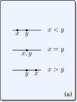
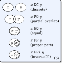
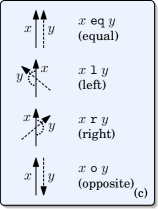
Figure 4: Illustration of the base relations for the calculi (a) $\mbox{{PC}}_{1}$, (b) RCC-5, and (c) CYC_b

Example 3.2.

The calculus RCC-5 [randell-cui-cohn-KR:92] symbolically represents five binary topological relations between regions in space (which may model objects): “is discrete from”, “partially overlaps with”, “equals”, “is proper part of”, and “has proper part”, plus their unions and intersections, see Figure 4 (b). For this purpose, RCC-5 provides the relation symbols DC, PO, EQ, PP, and PPi. The latter two are each other’s converses; the first three are their own converses. The composition of DC and PO is $\{\texttt{DC},\texttt{PO},\texttt{PP}\}$ because, whenever region $x$ is disconnected from $y$ and $y$ partially overlaps with $z$, there are three possible configurations between $x$ and $z$: those represented by $\texttt{DC},\texttt{PO},\texttt{PP}$. $\bullet$

Example 3.3.

The calculus CYC_b [DBLP:journals/ai/IsliC00] symbolically represents four binary topological relations between orientations of points in the plane (which may model observers and their lines of vision): “equals”, “is opposite to”, and “is to the left/right of”, plus their unions and intersections, see Figure 4 (c). For this purpose, CYC_b provides the relation symbols e, o, l, and r. The latter two are each other’s converses; e and o are their own converses. The composition of l and r is $\{\texttt{e},\texttt{l},\texttt{r}\}$: whenever orientation $x$ is to the left of $y$ and $y$ is to the left of $z$, then $x$ can be equal to, to the left of, or to the right of $z$. $\bullet$

Depending on the properties postulated for converse and composition, notions of a calculus of varying strengths exist [DBLP:journals/ki/NebelS02, LigozatR04]. The algebraic properties of binary calculi are well-understood, see Section 4.

The main motivation for using ternary relations is the requirement of directly capturing relative frames of reference which occur in natural language semantics [Levinson03:space]. In these frames of reference, the location of a target object is described from the perspective of an observer with respect to a reference object. For example, a hiker may describe a mountain peak to be to the left of a lake with respect to her own point of view. Another important motivation is the ability to express that an object is located between two others. Thus, ternary calculi typically contain projective relations for describing relative orientation and/or betweenness. The commitment to ternary (or $n$-ary) relations complicates matters significantly: instead of a single converse operation, there are now five (or $n!-1$) nontrivial permutation operations, and there is no longer a unique choice for a natural composition operation. For capturing the algebraic structure of $n$-ary relations, Condotta2006 proposed an algebra but there are other arguably natural choices, and they lead to different algebraic properties, as shown in Section 4. These difficulties may be the main reason why algebraic properties of ternary calculi are not as deeply studied as for binary calculi. Fortunately, this will not prevent us from establishing our general notion of a qualitative spatial (or temporal) calculus with relation symbols of arbitrary arity. However, we will then restrict our algebraic study to binary calculi; a unifying algebraic framework for $n$-ary calculi has yet to be established.

3.1 Requirements to Qualitative Spatial and Temporal Calculi

We start with minimal requirements used in the literature. We use the following standard notation. A universe is a non-empty set ${\mathord{\mathcal{U}}}$. With $X^{n}$ we denote the set of all $n$-tuples with elements from $X$. An $n$-ary domain relation is a subset $r\subseteq{\mathord{\mathcal{U}}}^{n}$. We use the prefix notation $r(x_{1},\dots,x_{n})$ to express $(x_{1},\dots,x_{n})\in r$; in the binary case we will often use the infix notation $x\,r\,y$ instead of $r(x,y)$.

Abstract partition schemes

LigozatR04 note that most spatial and temporal calculi are based on a set of JEPD (jointly exhaustive and pairwise disjoint) domain relations. The following definition is predominant in the QSTR literature [LigozatR04, Cohn:2008vn].

Definition 3.4.

Let ${\mathord{\mathcal{U}}}$ be a universe and ${\mathord{\mathcal{R}}}$ a set of non-empty domain relations of the same arity $n$. ${\mathord{\mathcal{R}}}$ is called a set of JEPD relations over ${\mathord{\mathcal{U}}}$ if the relations in ${\mathord{\mathcal{R}}}$ are jointly exhaustive, i.e., ${\mathord{\mathcal{U}}}^{n}=\bigcup_{r\in{\mathord{\mathcal{R}}}}r$, and pairwise disjoint.

An $n$-ary abstract partition scheme is a pair $({\mathord{\mathcal{U}}},{\mathord{\mathcal{R}}})$ where ${\mathord{\mathcal{R}}}$ is a set of JEPD relations over the universe ${\mathord{\mathcal{U}}}$. The relations in ${\mathord{\mathcal{R}}}$ are called base relations.

Example 3.5.

The calculus $\mbox{{PC}}_{1}$ is based on the binary abstract partition scheme $\mathcal{S}(\mbox{{PC}}_{1}):=(\mathbb{R},\{<,=,>\})$ where $\mathbb{R}$ is the set of reals and $\{<,=,>\}$ is clearly JEPD. For RCC-5, the universe is often chosen to be the set of all regular closed subsets of the 2- or 3-dimensional space $\mathbb{R}^{2}$ or $\mathbb{R}^{3}$. The five base relations from Figure 4 (b) are JEPD. For CYC_b, the universe is the set of all oriented line segments in the plane $\mathbb{R}^{2}$, given by angles between 0° and 360°. The four base relations from Figure 4 (c) are JEPD. $\bullet$

In Definition 3.4, the universe ${\mathord{\mathcal{U}}}$ represents the set of all spatial (or temporal) entities. The main ingredients of a calculus will be relation symbols representing the base relations in the underlying partition scheme. A constraint linking an $n$-tuple $t$ of entities via a relation symbol will thus represent complete information (modulo the qualitative abstraction underlying the partition scheme) about $t$. Incomplete information is modeled by $t$ being in a composite relation, which is a set of relation symbols representing the union of the corresponding base relations. The set of all relation symbols represents the universal relation (the union of all base relations) and indicates that no information is available.

Example 3.6.

In $\mbox{{PC}}_{1}$, “$x\texttt{\leavevmode\nobreak\ <\leavevmode\nobreak\ }y$” represents the relationship $a<b$, which holds complete information because $<$ is atomic in $\mathcal{S}(\mbox{{PC}}_{1})$. The statement “$x\leavevmode\nobreak\ \{\texttt{<},\texttt{=}\}\leavevmode\nobreak\ y$” represents the coarser relationship $a\leqslant b$ holding the incomplete information “$a<b$ or $a=b$”. Clearly “$x\leavevmode\nobreak\ \{\texttt{<},\texttt{=},\texttt{>}\}\leavevmode\nobreak\ y$” holds no information: “$a<b$ or $a=b$ or $a>b$” is always true. $\bullet$

The requirement that all base relations are JEPD ensures that every $n$-tuple of entities belongs to exactly one base relation. Thanks to PD (pairwise disjointness), there is a unique way to represent any composite relation using relation symbols and, due to JE (joint exhaustiveness), the empty relation can never occur in a consistent set of constraints, which is relevant for reasoning, see Section 3.2.

Example 3.7.

Consider the modification $\mbox{{PC}}_{1}^{\prime}$ based on the non-PD set $\{\leqslant,\geqslant\}$. Then the relationship $a=b$ can be expressed in two ways using relation symbols <= and >= representing $\leqslant$ and $\geqslant$: “$x\texttt{\leavevmode\nobreak\ <=\leavevmode\nobreak\ }y$” and “$x\texttt{\leavevmode\nobreak\ >=\leavevmode\nobreak\ }y$”.

Conversely, consider the variant $\mbox{{PC}}_{1}^{\prime\prime}$ based on the non-JE set $\{<,>\}$. Then the constraint $a=b$ cannot be expressed. Therefore, in any given set of constraints where it is known that $x,y$ stand for identical entities, we would find the empty relation between $x,y$. The standard reasoning procedure described in Section 3.2 would declare such sets of constraints to be inconsistent, although they are not – we have simply not been able to express $x=y$. $\bullet$

Partition schemes, identity, and converse

LigozatR04 base their definition of a (binary) qualitative calculus on the notion of a partition scheme, which imposes additional requirements on an abstract partition scheme. In particular, it requires that the set of base relations contains the identity relation and is closed under the converse operation. The analogous definition by Condotta2006 captures relations of arbitrary arity. Before we define the notion of a partition scheme, we discuss the generalization of identity and converse to the $n$-ary case.

The binary identity relation is given as usual by

$${\mathord{\textup{{id}}}}^{2}=\{(u,u)\mid u\in{\mathord{\mathcal{U}}}\}.$$ (1)

Example 3.8.

Clearly, $=$ in $\mathcal{S}(\mbox{{PC}}_{1})$ and “equals” in $\mathcal{S}(\mbox{{RCC-5}})$ and $\mathcal{S}(\mbox{{CYC}}_{b})$ are the identity relation over the respective domain. $\bullet$

The most inclusive way to generalize (1) to the $n$-ary case is to fix a set $M$ of numbers of all positions where tuples in ${\mathord{\textup{{id}}}}^{n}$ are required to agree. Thus, an $n$-ary identity relation is a domain relation ${\mathord{\textup{{id}}}}^{n}_{M}$ with $M\subseteq\{1,\dots,n\}$ and $|M|\geqslant 2$, which is defined by

$${\mathord{\textup{{id}}}}^{n}_{M} =\{(u_{1},\dots,u_{n})\in{\mathord{\mathcal{U}}}^{n}\mid u_{i}=u_{j}\text{\leavevmode\nobreak\ for all $i,j\in M$}\}.$$

This definition subsumes the “diagonal elements” $\Delta_{ij}$ of Condotta2006 for the case $|M|=2$. However, it is not enough to restrict attention to $|M|=2$ because there are ternary calculi which contain all identities ${\mathord{\textup{{id}}}}^{3}_{1,2}$, ${\mathord{\textup{{id}}}}^{3}_{1,3}$, ${\mathord{\textup{{id}}}}^{3}_{2,3}$, and ${\mathord{\textup{{id}}}}^{3}_{1,2,3}$, an example being the LR calculus, which was described as “the finest of its class” [SN05]. Since the relations in an $n$-ary abstract partition scheme are JEPD, all identities ${\mathord{\textup{{id}}}}^{n}_{M}$ are either base relations or subsumed by those. The stronger notion of a partition scheme should thus require that all identities be made explicit.

For binary relations, ${\mathord{\textup{{id}}}}^{2}$ from (1) is the unique identity relation ${\mathord{\textup{{id}}}}^{2}_{\{1,2\}}$.

The standard definition for the converse operation $\breve{\leavevmode\nobreak\ }$ on binary relations is

$$r\breve{\leavevmode\nobreak\ }=\{(v,u)\mid(u,v)\in r\}.$$ (2)

Example 3.9.

In $\mathcal{S}(\mbox{{PC}}_{1})$ we have that $\mathord{<}\breve{\leavevmode\nobreak\ }$ is $\mathord{>}$;  $\mathord{=}\breve{\leavevmode\nobreak\ }$ is $\mathord{=}$;  $\mathord{>}\breve{\leavevmode\nobreak\ }$ is $\mathord{<}$. The converses of the base relations in $\mathcal{S}(\mbox{{RCC-5}})$ and $\mathcal{S}(\mbox{{CYC}}_{b})$ were named in Examples 3.2 and 3.3. $\bullet$

In order to generalize the reversal of the pairs $(u,v)$ in (2) to $n$-ary tuples, we consider arbitrary permutations of $n$-tuples. An $n$-ary permutation is a bijection $\pi:\{1,\dots,n\}\to\{1,\dots,n\}$. We use the notation $\pi:(1,\dots,n)\mapsto(i_{1},\dots,i_{n})$ as an abbreviation for “$\pi(1)=i_{1}$, …, $\pi(n)=i_{n}$”. The identity permutation $\iota:(1,\dots,n)\mapsto(1,\dots,n)$ is called trivial; all other permutations are nontrivial.

A finite set $P$ of $n$-ary permutations is called generating if each $n$-ary permutation is a composition of permutations from $P$. For example, the following two permutations form a (minimal) generating set:

$${\mathord{\textup{{sc}}}} :(1,\dots,n)\mapsto(2,\dots,n,1)$$ (shortcut)

$${\mathord{\textup{{hm}}}} :(1,\dots,n)\mapsto(1,\dots,n-2,n,n-1)$$ (homing)

The names have been introduced in FZ92utilization for ternary permutations, together with a name for a third distinguished permutation:

$${\mathord{\textup{{inv}}}} :(1,\dots,n)\mapsto(2,1,3\dots,n)$$ (inversion)

Condotta2006 call shortcut “rotation” ($r^{\curvearrowright}$) and homing “permutation” ($r^{\looparrowright}$).

Example 3.10.

In Figure 5 we depict the permutations ${\mathord{\textup{{sc}}}}$ (rotation), ${\mathord{\textup{{hm}}}}$ (permutation), and ${\mathord{\textup{{inv}}}}$  for one relation from the ternary Double Cross Calculus (2-cross) [FZ92utilization]. The 2-cross relations specify the location of a point $P_{3}$ relative to an oriented line segment given by two points $P_{1},P_{2}$. Figure 5 a shows the relation right-front. The relations resulting from applying the permutations are depicted in Figure 5 b; e.g., ${\mathord{\textup{{sc}}}}(\texttt{right-front})=\texttt{right-back}$ because the latter is $P_{1}$’s position relative to the line segment $\overrightarrow{P_{2}P_{3}}$. Figure 5 c will be relevant later.

Figure 5:  (a) The 2-cross relation right-front;  (b) permutations of right-front;  (c) the composition $\texttt{right-front}\circ\texttt{right-front}$

For $n=2$, ${\mathord{\textup{{sc}}}}$, ${\mathord{\textup{{hm}}}}$ and ${\mathord{\textup{{inv}}}}$ coincide; indeed, there is a unique minimal generating set, which consists of the single permutation $\breve{\leavevmode\nobreak\ }:(1,2)\mapsto(2,1)$. For $n\geqslant 3$, there are several generating sets, e.g., $\{{\mathord{\textup{{sc}}}},{\mathord{\textup{{hm}}}}\}$ and $\{{\mathord{\textup{{inv}}}},{\mathord{\textup{{hm}}}}\}$.

Now an $n$-ary permutation operation is a map $\cdot^{\pi}$ that assigns to each $n$-ary domain relation $r$ an $n$-ary domain relation denoted by $r^{\pi}$, where $\pi$ is an $n$-ary permutation and the following holds: $r^{\pi}=\{(u_{\pi(1)},\dots,u_{\pi(n)})\mid(u_{1},\dots,u_{n})\in r\}$

We are now ready to give our definition of a partition scheme, lifting Ligozat and Renz’s binary version to the $n$-ary case, and generalizing Condotta et al.’s $n$-ary version to arbitrary generating sets.

Definition 3.11.

An $n$-ary partition scheme $({\mathord{\mathcal{U}}},{\mathord{\mathcal{R}}})$ is an $n$-ary abstract partition scheme with the following two additional properties.

1. ${\mathord{\mathcal{R}}}$ contains all identity relations ${\mathord{\textup{{id}}}}^{n}_{M}$, $M\subseteq\{1,\dots,n\}$, $|M|\geqslant 2$.

2. There is a generating set $P$ of permutations such that, for every $r\in{\mathord{\mathcal{R}}}$ and every $\pi\in P$, there is some $s\in{\mathord{\mathcal{R}}}$ with $r^{\pi}=s$.

In the special case of binary relations, we have the following.

Observation 3.12

A binary partition scheme $({\mathord{\mathcal{U}}},{\mathord{\mathcal{R}}})$ is a binary abstract partition scheme with the following two additional properties.

1. ${\mathord{\mathcal{R}}}$ contains the identity relation ${\mathord{\textup{{id}}}}^{2}$.

2. For every $r\in{\mathord{\mathcal{R}}}$, there is some $s\in{\mathord{\mathcal{R}}}$ such that $r\breve{\leavevmode\nobreak\ }=s$.

Example 3.13.

It follows that $\mathcal{S}(\mbox{{PC}}_{1})$, $\mathcal{S}(\mbox{{RCC-5}})$, and $\mathcal{S}(\mbox{{CYC}}_{b})$ are even partition schemes. In contrast, the abstract partition scheme $(\mathbb{R},\{\leqslant,>\})$ is not a partition scheme: it violates both conditions of Observation 3.12 (and thus of Definition 3.11). $\bullet$

Example 3.14.

As an example of an intuitive and useful abstract partition scheme that is not a partition scheme, consider the calculus Cardinal Direction Relations (CDR) [SkiadoK05]. CDR describes the placement of regions in a 2D space (e.g., countries on the globe) relative to each other, and with respect to a fixed coordinate system. The axes of the bounding box of the reference region $y$ divide the space into nine tiles, see Fig. 6 (a). The binary relations in $\mathcal{S}(\mbox{{CDR}})$ now determine which tiles relative to $y$ are occupied by a primary region $x$: e.g., in Fig. 6 (b), tiles N, W, and B of $y$ are occupied by $x$; hence we have $x$ N:W:B $y$. Simple combinatorics yields $2^{9}-1=511$ base relations.

Now $\mathcal{S}(\mbox{{CDR}})$ is not a partition scheme because it violates Condition 2 of Observation 3.12 (and thus of Definition 3.11): e.g., the converse of the base relation S (south) is not a base relation. To justify this claim, assume the contrary. Take two specific regions $x,y$ with $x$ S $y$, namely two unit squares, where $y$ is exactly above $x$. Then we also have $y$ N $x$; therefore the converse of S is N. Now stretch the width of $x$ by any factor $>1$. Then we still have $y$ N $x$, but no longer $x$ S $y$. Hence the converse of S cannot comprise all of N, which contradicts the assumption that the converse of S is a base relation.

The related calculus RCD [NavarreteEtAl13] abstracts away from the concrete shape of regions and replaces them with their bounding boxes, see Fig. 6 (c). $\mathcal{S}(\mbox{{RCD}})$ is not a partition scheme, with the same argument from above. $\bullet$

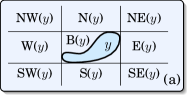
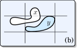
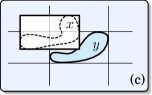
Figure 6: Calculi CDR and RCD: (a) reference tiles; (b) the CDR base relation $x$ N:W:B $y$; (c) the RCD base relation $x$ NW:N:W:B $y$

It is important to note that violations of Definition 3.11 such as those reported in Example 3.14 are not necessarily bugs in the design of the respective calculi – in fact they are often a feature of the corresponding representation language, which is deliberately designed to be just as fine as necessary, and may thus omit some identity relations or converses/compositions of base relations. To turn, say, CDR into a partition scheme, one would have to break down the 511 base relations into smaller ones, resulting in even more, less cognitively plausible ones. Thus violations of Definition 3.11 are unavoidable, and we adopt the more general notion of an abstract partition scheme.

Calculi

Intuitively, a qualitative spatial (or temporal) calculus is a symbolic representation of an abstract partition scheme and additionally represents the composition operation on the relations involved. As before, we need to discuss the generalization of binary composition to the $n$-ary case before we can define it precisely.

For binary domain relations, the standard definition of composition is:

$$r\circ s=\{(u,w)\mid\exists\underline{v}\in{\mathord{\mathcal{U}}}:(u,\underline{v})\in r\text{ and }(\underline{v},w)\in s\}$$ (3)

Example 3.15.

In $\mathcal{S}(\mbox{{PC}}_{1})$ we have, e.g., that $\mathord{<}\circ\mathord{<}$ equals $\mathord{<}$ because $a<b$ and $b<c$ imply $a<c$. Furthermore, $\mathord{<}\circ\mathord{>}$ yields the universal relation, i.e., the union of $<$, $=$, and $>$, because “$a<b$ and $b>c$” is consistent with each of $a<c$, $a=c$, and $a>c$. $\bullet$

We are aware of three ways to generalize (3) to higher arities. The first is a binary operation on the ternary relations of the calculus 2-cross [Freksa92, FZ92utilization], see also Fig. 5:

$$r\mathbin{\circ^{3}_{\text{FZ}}}s=\{(u,v,w)\mid\exists\underline{x}:(u,v,\underline{x})\in r\text{ and }(v,\underline{x},w)\in s\}$$

It says: if the location of $x$ relative to $u$ and $v$ is determined by $r$ and the location of $w$ relative to $v$ and $x$ is determined by $s$, then the location of $w$ relative to $u$ and $v$ is determined by $r\mathbin{\circ^{3}_{\text{FZ}}}s$. Fig. 5 c shows the composition of the 2-cross relation right-front with itself; i.e., $\texttt{right-front}\mathbin{\circ^{3}_{\text{FZ}}}\texttt{right-front}$. The red area indicates the possible locations of the point $P_{4}$; hence the resulting relation is $\{\texttt{right-front},\texttt{right-middle},\texttt{right-back}\}$. A generalization to other calculi and arities $n>3$ is obvious.

A second alternative results in $n(n-1)$ binary operations $\mathbin{{}_{i}\circ_{j}^{n}}$ [DBLP:journals/ai/IsliC00, SN05]: the composition of $r$ and $s$ consists of those $n$-tuples that belong to $r$ (respectively, $s$) if the $i$-th (respectively, $j$-th) component is replaced by some uniform element $v$.

$$r\mathbin{{}_{i}\circ_{j}^{n}}s=\{(u_{1},\dots,u_{n})\mid\exists\underline{v}:\leavevmode\nobreak\ (u_{1},\dots,u_{i-1},\underline{v},u_{i+1},\dots,u_{n})\in r\text{ and }$$

$$(u_{1},\dots,u_{j-1},\underline{v},u_{j+1},\dots,u_{n})\in s\qquad\}$$

In the ternary case, this yields, for example:

$$r\mathbin{{}_{3}\circ_{2}^{3}}s=\{(u,v,w)\mid\exists\underline{x}:(u,v,\underline{x})\in r\text{ and }(u,\underline{x},w)\in s\}$$ (4)

If we assume, for example, that the underlying partition scheme speaks about the relative position of points, we can consider (4) to say: if the position of $x$ relative to $u$ and $v$ is determined by the relation $r$ (as given by $(u,v,x)\in r$) and the position of $w$ relative to $u$ and $x$ is determined by the relation $s$ (as given by $(u,x,w)\in s$), then the position of $w$ relative to $u$ and $v$ can be inferred to be determined by $r\mathbin{{}_{3}\circ_{2}^{3}}s$.

The third is perhaps the most general, resulting in an $n$-ary operation [Condotta2006]: $\circ(r_{1},\dots,r_{n})$ consists of those $n$-tuples which, for every $i=1,\dots,n$, belong to the relation $r_{i}$ whenever their $i$-th component is replaced by some uniform $v$.

$$\circ(r_{1},\dots,r_{n})=\{ (u_{1},\dots,u_{n})\mid\exists\underline{v}\in{\mathord{\mathcal{U}}}:(u_{1},\dots,u_{n-1},\underline{v})\in r_{1}\leavevmode\nobreak\ \text{and}\leavevmode\nobreak\$$

$$(u_{1},\dots,u_{n-2},\underline{v},u_{n})\in r_{2}\leavevmode\nobreak\ \text{and}\leavevmode\nobreak\ \dots\leavevmode\nobreak\ \text{and}\leavevmode\nobreak\ (\underline{v},u_{2},\dots,u_{n})\in r_{n}\}$$ (5)

As an example, consider again $n=3$ and 2-cross. Equation (5) says that the composition result of the relations right-front, right-front, and left-back is the set of all triples $(u_{1},u_{2},u_{3})$ such that there is an element $v$ with $(u_{1},u_{2},v)\in\texttt{right-front}$, $(u_{1},v,u_{3})\in\texttt{right-front}$, and $(v,u_{2},u_{3})\in\texttt{right-back}$. That set is exactly the relation right-front, which can be seen drawing pictures similar to Fig. 5.

For binary domain relations, all these alternative approaches collapse to (3).

In the light of the diverse views on composition, we define a composition operation on $n$-ary domain relations to be an operation of arity $2\leqslant m\leqslant n$ on $n$-ary domain relations, without imposing additional requirements. Those are not necessary for the following definitions, which are independent of the particular choice of composition.

We now define our minimal notion of a spatial calculus, which provides a set of symbols for the relations in an abstract partition scheme (${\mathord{\textup{{Rel}}}}$), and for some choice of nontrivial permutation operations ($\breve{\leavevmode\nobreak\ }^{1},\dots,\breve{\leavevmode\nobreak\ }^{k}$) and some composition operation ($\diamond$).

Definition 3.16.

An $n$-ary qualitative calculus is a tuple $({\mathord{\textup{{Rel}}}},{\mathord{\textup{{Int}}}},\breve{\leavevmode\nobreak\ }^{1},\dots,\breve{\leavevmode\nobreak\ }^{k},\diamond)$ with $k\geqslant 1$ and the following properties.

• ${\mathord{\textup{{Rel}}}}$ is a finite, non-empty set of $n$-ary relation symbols (denoted $r,s,t,\dots$). The subsets of ${\mathord{\textup{{Rel}}}}$, including singletons, are called composite relations (denoted $R,S,T,\dots$).

• ${\mathord{\textup{{Int}}}}=({\mathord{\mathcal{U}}},\varphi,\cdot^{\pi_{1}},\dots,\cdot^{\pi_{k}},\circ)$ is an interpretation with the following properties.

  • ${\mathord{\mathcal{U}}}$ is a universe.

  • $\varphi:{\mathord{\textup{{Rel}}}}\to 2^{{\mathord{\mathcal{U}}}^{n}}$ is an injective map assigning an $n$-ary relation over ${\mathord{\mathcal{U}}}$ to each relation symbol, such that $({\mathord{\mathcal{U}}},\{\varphi(r)\mid r\in{\mathord{\textup{{Rel}}}}\})$ is an abstract partition scheme. The map $\varphi$ is extended to composite relations $R\subseteq{\mathord{\textup{{Rel}}}}$ by setting $\varphi(R)=\bigcup_{r\in R}\varphi(r)$.

  • $\{\cdot^{\pi_{1}},\dots,\cdot^{\pi_{k}}\}$ is a set of $n$-ary nontrivial permutation operations.

  • $\circ$ is a composition operation on $n$-ary domain relations that has arity $2\leqslant m\leqslant n$.

• Every permutation operation $\breve{\leavevmode\nobreak\ }^{i}$ is a map $\breve{\leavevmode\nobreak\ }^{i}:{\mathord{\textup{{Rel}}}}\to 2^{\mathord{\textup{{Rel}}}}$ that satisfies

  $$\varphi(r\breve{\leavevmode\nobreak\ }^{i})\supseteq\varphi(r)^{\pi_{i}}$$ (6)

  for every $r\in{\mathord{\textup{{Rel}}}}$. The operation $\breve{\leavevmode\nobreak\ }^{i}$ is extended to composite relations $R\subseteq{\mathord{\textup{{Rel}}}}$ by setting $R\breve{\leavevmode\nobreak\ }^{i}=\bigcup_{r\in R}r\breve{\leavevmode\nobreak\ }^{i}$.

• The composition operation $\diamond$ is a map $\diamond:{\mathord{\textup{{Rel}}}}^{m}\to 2^{\mathord{\textup{{Rel}}}}$ that satisfies

  $$\varphi(\diamond(r_{1},\dots,r_{m}))\supseteq\circ(\varphi(r_{1}),\dots,\varphi(r_{m}))$$ (7)

  for all $r_{1},\dots,r_{m}\in{\mathord{\textup{{Rel}}}}$. The operation $\diamond$ is extended to composite relations $R_{1},\dots,R_{m}\subseteq{\mathord{\textup{{Rel}}}}$ by setting $\diamond(R_{1},\dots,R_{m})=\bigcup_{r_{1}\in R_{1}}\dots\bigcup_{r_{m}\in R_{m}}\diamond(r_{1},\dots,r_{m})$.

In the special case of binary relations, the natural converse is the only non-trivial permutation operation. Hence $k=1$ and we have the following.

Observation 3.17

A binary qualitative calculus is a tuple $({\mathord{\textup{{Rel}}}},{\mathord{\textup{{Int}}}},\breve{\leavevmode\nobreak\ },\diamond)$ with the following properties.

• ${\mathord{\textup{{Rel}}}}$ is as in Definition 3.16.

• ${\mathord{\textup{{Int}}}}=({\mathord{\mathcal{U}}},\varphi,\pi,\circ)$ is an interpretation with the following properties.

  • ${\mathord{\mathcal{U}}}$ is a universe.

  • $\varphi:{\mathord{\textup{{Rel}}}}\to 2^{{\mathord{\mathcal{U}}}\times{\mathord{\mathcal{U}}}}$ is an injective map as in Definition 3.16.

  • $\pi$ is the standard converse operation on binary domain relations from (2).

  • $\circ$ is the standard composition operation on binary domain relations from (3).

• The converse operation $\breve{\leavevmode\nobreak\ }$ is a map $\breve{\leavevmode\nobreak\ }:{\mathord{\textup{{Rel}}}}\to 2^{\mathord{\textup{{Rel}}}}$ that satisfies

  $$\forall r\in{\mathord{\textup{{Rel}}}}:\quad\varphi(r\breve{\leavevmode\nobreak\ })\supseteq\varphi(r)^{\pi}\,.$$

• The composition operation $\diamond$ is a map $\diamond:{\mathord{\textup{{Rel}}}}\times{\mathord{\textup{{Rel}}}}\to 2^{\mathord{\textup{{Rel}}}}$ that satisfies

  $$\forall r,s\in{\mathord{\textup{{Rel}}}}:\quad\varphi(\diamond(r,s))\supseteq\circ(\varphi(r),\varphi(s))\,.$$

Due to the last sentence of Definition 3.16, the composition operation of a calculus is uniquely determined by the composition of each pair of relation symbols. This information is usually stored in an $m$-dimensional table, the composition table.

Example 3.18.

We can now observe that $\mbox{{PC}}_{1}$ is indeed a binary calculus with the following components.

• The set of relation symbols is ${\mathord{\textup{{Rel}}}}=\{\texttt{<},\texttt{=},\texttt{>}\}$, denoting the relations depicted in Figure 4 a. The $2^{3}=8$ composite relations include, for example, $R_{1}=\{\texttt{<},\texttt{=}\}$ and $R_{2}=\{\texttt{<},\texttt{=},\texttt{>}\}$.

• There are several possible interpretations, depending largely on the chosen universe. One of the most natural choices leads to the interpretation ${\mathord{\textup{{Int}}}}=\{{\mathord{\mathcal{U}}},\varphi,\pi,\circ\}$ with the following components.

  • The universe ${\mathord{\mathcal{U}}}$ is the set of reals.

  • The map $\varphi$ maps <, =, and > to $<$, $=$, and $>$, respectively; see Figure 4 a. Its extension to composite relations maps, for example, $R_{1}$ from above to $\geqslant$ and $R_{2}$ to the universal relation.

  • The operations $\pi$ and $\circ$ are the standard binary converse and composition operations from (2) and (3).

• The converse operation $\breve{\leavevmode\nobreak\ }$ is given by Table 1 a. For its extension to composite relations, we have, e.g., $R_{1}\breve{\leavevmode\nobreak\ }=\{\texttt{>},\texttt{=}\}$ and $R_{2}\breve{\leavevmode\nobreak\ }=R_{2}$.

  (a)   $r$ $r\breve{\leavevmode\nobreak\ }$ < > = = > <

  (b)   r\s   <   =   > < $\{\texttt{<}\}$ $\{\texttt{<}\}$ $\{\texttt{<},\texttt{=},\texttt{>}\}$ = $\{\texttt{<}\}$ $\{\texttt{=}\}$ $\{\texttt{>}\}$ > $\{\texttt{<},\texttt{=},\texttt{>}\}$ $\{\texttt{>}\}$ $\{\texttt{>}\}$

  Table 1: Converse and composition tables for the point calculus $\mbox{{PC}}_{1}$.

• The composition operation $\diamond$ is given by a $3\times 3$ table where each cell represents $r\diamond s$, see Table 1 b. For its extension to composite relations, we have, for example:

  $$R_{1}\diamond R_{2} =\{\texttt{<},\texttt{=}\}\diamond\{\texttt{<},\texttt{=},\texttt{>}\}$$

  $$=\{\texttt{<}\}\diamond\{\texttt{<}\}\leavevmode\nobreak\ \cup\leavevmode\nobreak\ \{\texttt{<}\}\diamond\{\texttt{=}\}\leavevmode\nobreak\ \cup\leavevmode\nobreak\ \dots\leavevmode\nobreak\ \cup\leavevmode\nobreak\ \{\texttt{=}\}\diamond\{\texttt{>}\}$$

  $$=\{\texttt{<}\}\cup\{\texttt{<}\}\cup\dots\cup\{\texttt{>}\}$$

  $$=R_{2}$$

  $\bullet$

Example 3.19.

RCC-5 too is a binary calculus, with the following components.

• The set of relation symbols is ${\mathord{\textup{{Rel}}}}=\{\texttt{EQ},\texttt{DC},\texttt{PO},\texttt{PP},\texttt{PPi}\}$, denoting the relations depicted in Figure 4 b. The $2^{5}=32$ composite relations include, for example, $R_{1}=\{\texttt{DC},\texttt{PO},\texttt{PP},\texttt{PPi}\}$ (“both regions are distinct”) and $R_{2}=\{\texttt{PP},\texttt{PPi}\}$ (“one region is a proper part of the other”).

• Similarly to $\mbox{{PC}}_{1}$, there are several possible interpretations, a natural choice being ${\mathord{\textup{{Int}}}}=\{{\mathord{\mathcal{U}}},\varphi,\pi,\circ\}$ with the following components.

  • The universe ${\mathord{\mathcal{U}}}$ is the set of all regular closed subsets of $\mathbb{R}^{2}$.

  • The map $\varphi$ maps, for example, DC to all pairs of regions that are disconnected or externally connected. Figure 4 b illustrates $\varphi(r)$ for all relation symbols $r=\texttt{EQ},\texttt{DC},\texttt{PO},\texttt{PP},\texttt{PPi}$.

  • The operations $\pi$ and $\circ$ are the standard binary converse and composition operations from (2) and (3).

• The converse operation $\breve{\leavevmode\nobreak\ }$ is given by Table 2 a. we have, e.g., $R_{2}\breve{\leavevmode\nobreak\ }=R_{2}$.

  (a)   $r$ $r\breve{\leavevmode\nobreak\ }$ EQ EQ DC DC PO PO PP PP PPi PPi

  (b)   r\s   EQ   DC   PO   PP   PPi EQ $\{\texttt{EQ}\}$ $\{\texttt{DC}\}$ $\{\texttt{PO}\}$ $\{\texttt{PO}\}$ $\{\texttt{PPi}\}$ DC $\{\texttt{DC}\}$ $\{\texttt{EQ},\texttt{DC},\texttt{PO},\texttt{PP},\texttt{PPi}\}$ $\{\texttt{DC},\texttt{PO},\texttt{PP}\}$ $\{\texttt{DC},\texttt{PO},\texttt{PP}\}$ $\{\texttt{DC}\}$ PO $\{\texttt{PO}\}$ $\{\texttt{DC},\texttt{PO},\texttt{PPi}\}$ $\{\texttt{EQ},\texttt{DC},\texttt{PO},\texttt{PP},\texttt{PPi}\}$ $\{\texttt{PO},\texttt{PP}\}$ $\{\texttt{DC},\texttt{PO},\texttt{PPi}\}$ PP $\{\texttt{PP}\}$ $\{\texttt{DC}\}$ $\{\texttt{DC},\texttt{PO},\texttt{PP}\}$ $\{\texttt{PP}\}$ $\{\texttt{EQ},\texttt{DC},\texttt{PO},\texttt{PP},\texttt{PPi}\}$ PPi $\{\texttt{PPi}\}$ $\{\texttt{DC},\texttt{PO},\texttt{PPi}\}$ $\{\texttt{PO},\texttt{PPi}\}$ $\{\texttt{EQ},\texttt{PO},\texttt{PP},\texttt{PPi}\}$ $\{\texttt{PPi}\}$

  Table 2: Converse and composition tables for the point calculus RCC-5.

• The composition operation $\diamond$ is given by a $5\times 5$ table where each cell represents $r\diamond s$, see Table 2 b. For its extension to composite relations, we have, for example:

  $$\{\texttt{PP},\texttt{PPi}\}\diamond\{\texttt{DC}\} =\{\texttt{PP}\}\diamond\{\texttt{DC}\}\leavevmode\nobreak\ \cup\leavevmode\nobreak\ \{\texttt{PPi}\}\diamond\{\texttt{DC}\}$$

  $$=\{\texttt{DC}\}\leavevmode\nobreak\ \cup\leavevmode\nobreak\ \{\texttt{DC},\texttt{PO},\texttt{PPi}\}$$

  $$=\{\texttt{DC},\texttt{PO},\texttt{PPi}\}$$

  $\bullet$

Example 3.20.

CYC_b too is a binary calculus, with the following components.

• The set of relation symbols is ${\mathord{\textup{{Rel}}}}=\{\texttt{e},\texttt{o},\texttt{l},\texttt{r}\}$, denoting the relations depicted in Figure 4 c. The $2^{4}=16$ composite relations include, for example, $R_{1}=\{\texttt{e},\texttt{l}\}$ (“the orientation $y$ is to the left of, or equal to, $x$”) and $R_{2}=\{\texttt{e},\texttt{o}\}$ (“both orientations are equal or opposite to each other”).

• The standard interpretation for CYC_b is ${\mathord{\textup{{Int}}}}=\{{\mathord{\mathcal{U}}},\varphi,\pi,\circ\}$ with the following components.

  • The universe ${\mathord{\mathcal{U}}}$ is the set of all 2D-orientations, which can equivalently be viewed as either the set of radii of a given fixed circle $C$, or the set of points on the periphery of $C$, or the set of directed lines through a given fixed point (the origin of $C$).

  • The map $\varphi$ maps, for example, l to all pairs $(x,y)$ of directed lines where the angle $\alpha$ from $x$ to $y$, in counterclockwise fashion, satisfies $0^{\circ}<\alpha<180^{\circ}$. Analogously o is mapped to those pairs where that angle is exactly $180^{\circ}$. Figure 4 c illustrates $\varphi(r)$ for all relation symbols $r=\texttt{e},\texttt{o},\texttt{l},\texttt{r}$.

  • The operations $\pi$ and $\circ$ are the standard binary converse and composition operations from (2) and (3).

• The converse operation $\breve{\leavevmode\nobreak\ }$ is given by Table 3 a. For its extension to composite relations, we have, e.g., $R_{1}\breve{\leavevmode\nobreak\ }=\{\texttt{e},\texttt{l}\}$.

  (a)   $r$ $r\breve{\leavevmode\nobreak\ }$ e e o o l r r l

  (b)   r\s   e   o   l   r e $\{\texttt{e}\}$ $\{\texttt{o}\}$ $\{\texttt{l}\}$ $\{\texttt{r}\}$ o $\{\texttt{o}\}$ $\{\texttt{e}\}$ $\{\texttt{r}\}$ $\{\texttt{l}\}$ l $\{\texttt{l}\}$ $\{\texttt{r}\}$ $\{\texttt{l},\texttt{o},\texttt{r}\}$ $\{\texttt{e},\texttt{l},\texttt{r}\}$ r $\{\texttt{r}\}$ $\{\texttt{l}\}$ $\{\texttt{e},\texttt{l},\texttt{r}\}$ $\{\texttt{l},\texttt{o},\texttt{r}\}$

  Table 3: Converse and composition tables for the point calculus CYC_b.

• The composition operation $\diamond$ is given by a $4\times 4$ table where each cell represents $r\diamond s$, see Table 3 b. For its extension to composite relations, we have, for example:

  $$R_{1}\diamond R_{1} =\{\texttt{e},\texttt{l}\}\diamond\{\texttt{e},\texttt{l}\}$$

  $$=\{\texttt{e}\}\diamond\{\texttt{e}\}\leavevmode\nobreak\ \cup\leavevmode\nobreak\ \{\texttt{e}\}\diamond\{\texttt{l}\}\leavevmode\nobreak\ \cup\leavevmode\nobreak\ \{\texttt{l}\}\diamond\{\texttt{e}\}\leavevmode\nobreak\ \cup\leavevmode\nobreak\ \{\texttt{l}\}\diamond\{\texttt{l}\}$$

  $$=\{\texttt{e}\}\leavevmode\nobreak\ \cup\leavevmode\nobreak\ \{\texttt{l}\}\leavevmode\nobreak\ \cup\leavevmode\nobreak\ \{\texttt{l}\}\leavevmode\nobreak\ \cup\leavevmode\nobreak\ \{\texttt{e},\texttt{l},\texttt{r}\}$$

  $$=\{\texttt{e},\texttt{l},\texttt{r}\}$$

  $\bullet$

Abstract versus weak and strong operations

We call permutation and composition operations with Properties (6) and (7) abstract permutation and abstract composition, following Ligozat’s naming in the binary case [Lig05]. For reasons explained further below, our notion of a qualitative calculus imposes weaker requirements on the permutation operation than Ligozat and Renz’s notions of a weak (binary) representation [Lig05, LigozatR04] or the notion of a (binary) constraint algebra [DBLP:journals/ki/NebelS02]. The following definition specifies those stronger variants, see, e.g., LigozatR04.

Definition 3.21.

Let $({\mathord{\textup{{Rel}}}},{\mathord{\textup{{Int}}}},\breve{\leavevmode\nobreak\ }^{1},\dots,\breve{\leavevmode\nobreak\ }^{k},\diamond)$ be a qualitative calculus based on the interpretation ${\mathord{\textup{{Int}}}}=({\mathord{\mathcal{U}}},\varphi,\cdot^{\pi_{1}},\dots,\cdot^{\pi_{k}},\circ)$.

The permutation operation $\breve{\leavevmode\nobreak\ }^{i}$ is a weak permutation if, for all $r\in{\mathord{\textup{{Rel}}}}$:

$$r\breve{\leavevmode\nobreak\ }^{i}=\bigcap\{S\subseteq{\mathord{\textup{{Rel}}}}\mid\varphi(S)\supseteq\varphi(r)^{\pi_{i}}\}$$ (8)

The permutation operation $\breve{\leavevmode\nobreak\ }^{i}$ is a strong permutation if, for all $r\in{\mathord{\textup{{Rel}}}}$:

$$\varphi(r\breve{\leavevmode\nobreak\ }^{i})=\varphi(r)^{\pi_{i}}$$ (9)

The composition operation $\diamond$ is a weak composition if, for all $r_{1},\dots,r_{m}\in{\mathord{\textup{{Rel}}}}$:

$$\diamond(r_{1},\dots,r_{m})=\bigcap\{S\subseteq{\mathord{\textup{{Rel}}}}\mid\varphi(S)\supseteq\circ(\varphi(r_{1}),\dots,\varphi(r_{m}))\}$$ (10)

The composition $\diamond$ is a strong composition if, for all $r_{1},\dots,r_{m}\in{\mathord{\textup{{Rel}}}}$:

$$\varphi(\diamond(r_{1},\dots,r_{m}))=\circ(\varphi(r_{1}),\dots,\varphi(r_{m}))$$ (11)

In the literature, the equivalent variant $r\breve{\leavevmode\nobreak\ }^{i}=\{s\in{\mathord{\textup{{Rel}}}}\mid\varphi(s)\cap\varphi(r)^{\pi_{i}}\neq\emptyset\}$ of Equation (8) is sometimes found; analogously for Equation (10).

Example 3.22.

The converse and permutation operation in $\mbox{{PC}}_{1}$ are both strong because (9) holds for all three relation symbols (e.g., $\varphi(\texttt{<}\breve{\leavevmode\nobreak\ })=\varphi(\texttt{>})=\mathord{>}=\mathord{<}\breve{\leavevmode\nobreak\ }=\varphi(\texttt{<})\breve{\leavevmode\nobreak\ }$), and the binary version of (11), namely

$$\varphi(r_{1}\diamond r_{2})=\varphi(r_{1})\circ\varphi(r_{2}),$$

holds for all nine pairs of relation symbols (e.g., $\varphi(\texttt{>}\diamond\texttt{>})=\varphi(\texttt{>})=\mathord{>}=\mathord{>}\circ\mathord{>}=\varphi(\texttt{>})\circ\varphi(\texttt{>})$). $\bullet$

Example 3.23.

Consider the variant $\mbox{{PC}}_{1}^{\mathbb{N}}$ of $\mbox{{PC}}_{1}$ that is interpreted over the universe $\mathbb{N}$. It contains the same base relations with the usual interpretation and, obviously, the same converse operation, see Example 3.18. However, composition is no longer strong because $\mathord{<}\circ\mathord{<}\subsetneq\mathord{<}$ holds: for “$\subseteq$” observe that, whenever $x<y<z$ for three points $x,y,z\in\mathbb{N}$, it follows that $x<z$; and “$\nsupseteq$” holds because there are points $x,z$ with $x<z$ for which there is no $y$ with $x<y<z$, for example, $x=0$, $z=1$. More precisely, the result of the composition $\texttt{<}\diamond\texttt{<}$ should be the relation $<^{1}=\{(x,z)\mid x+1<z\}$. Since $<^{1}$ is not expressible by a union of base relations, we cannot endow this calculus with a strong symbolic composition operation. Consequently we have a choice as to the composition result in question. Regardless of that choice, the composition table will incur a loss of information because it cannot capture that the pair $(x,z)$ is in $<^{1}$.

If we opt for weak composition, then Equation (10) requires us to generate the result of $\texttt{<}\diamond\texttt{<}$ from the symbols for exactly those relations that overlap with the domain-level composition $\mathord{<}\circ\mathord{<}$. From the above it is clear that this is exactly <. One can now easily check that, for the case of weak composition, we get precisely Table 2 b.

On the contrary, if we do not care about composition being weak, then abstract composition (Inequality (7)) requires us to generate the result of $\texttt{<}\diamond\texttt{<}$ from the symbols for at least those relations that overlap with $\mathord{<}\circ\mathord{<}$. This means that we can postulate $\texttt{<}\diamond\texttt{<}=\{\texttt{<}\}$ as before or, for example, $\texttt{<}\diamond\texttt{<}=\{\texttt{<},\texttt{=},\texttt{>}\}$.

The difference between weak and abstract composition is that abstract composition allows us to make the composition result arbitrarily general, whereas weak composition forces us to take exactly those relations into account that contain possible pairs of $(x,z)$. Weak composition therefore restricts the loss of information to an unavoidable minimum, whereas abstract composition does not provide such a guarantee: the more base relations are included in the composition result, the more information we lose on how $x$ and $z$ are interrelated.

In this connection, it becomes clear why we require composition to be at least abstract: without this requirement, we could omit, for example, < from the above composition result. This would result in adding spurious information because we would suddenly be able to conclude that the constellation $x<y<z$ is impossible, just because $\texttt{<}\diamond\texttt{<}=\emptyset$. This insight, in turn, is particularly important for ensuring soundness of the most common reasoning algorithm, a-closure, see Section 3.2. $\bullet$

In terms of composition tables, abstract composition requires that each cell corresponding to $\diamond(r_{1},\dots,r_{m})$ contains at least those relation symbols $t$ whose interpretation intersects with $\circ(\varphi(r_{1}),\dots,\varphi(r_{m}))$. Weak composition additionally requires that each cell contains exactly those $t$. Strong composition, in contrast, implies a requirement to the underlying partition scheme: whenever $\varphi(t)$ intersects with $\circ(\varphi(r_{1}),\dots,\varphi(r_{m}))$, it has to be contained in $\circ(\varphi(r_{1}),\dots,\varphi(r_{m}))$. Analogously for permutation.

These explanations and those in Example 3.23 show that abstractness as in Properties (6) and (7) captures minimal requirements to the operations in a qualitative calculus: it ensures that, whenever the symbolic relations cannot capture the converse or composition of some domain relations exactly, the symbolic converse (composition) approximates its domain-level counterpart from above, thus avoiding the introduction of spurious information. Weakness (Properties (8) and (10)) additionally ensures that the loss of information is kept to the unavoidable minimum. This last observation is presumably the reason why existing calculi (see Section 3.4) typically have at least weak operations – we are not aware of any calculus with only abstract operations.

In Section 3.2, we will see that abstract composition is a minimal requirement for ensuring soundness of the most common reasoning algorithm, a-closure, and review the impact of the various strengths of the operations on reasoning algorithms.

The three notions form a hierarchy:

Fact 1.

Every strong permutation (composition) is weak, and every weak permutation (composition) is abstract. $\lhd$ LABEL:app:abstract_vs_weak_vs_strong

It suffices to postulate the properties weakness and strongness with respect to relation symbols only: they carry over to composite relations as shown in Fact 2.

Fact 2.

Given a qualitative calculus $({\mathord{\textup{{Rel}}}},{\mathord{\textup{{Int}}}},\breve{\leavevmode\nobreak\ }^{1},\dots,\breve{\leavevmode\nobreak\ }^{k},\diamond)$ the following holds.

For all composite relations $R\subseteq{\mathord{\textup{{Rel}}}}$ and $i=1,\dots,k$:

$$\varphi(R\breve{\leavevmode\nobreak\ }^{i})\supseteq\varphi(R)^{\pi_{i}}$$ (12)

For all composite relations $R_{1},\dots,R_{m}\subseteq{\mathord{\textup{{Rel}}}}$:

$$\varphi(\diamond(R_{1},\dots,R_{m}))\supseteq\circ(\varphi(R_{1}),\dots,\varphi(R_{m}))$$ (13)

If $\breve{\leavevmode\nobreak\ }^{i}$ is a weak permutation, then, for all $R\subseteq{\mathord{\textup{{Rel}}}}$:

$$R\breve{\leavevmode\nobreak\ }^{i}=\bigcap\{S\subseteq{\mathord{\textup{{Rel}}}}\mid\varphi(S)\supseteq\varphi(R)^{\pi_{i}}\}$$

If $\breve{\leavevmode\nobreak\ }^{i}$ is a strong permutation, then, for all $R\subseteq{\mathord{\textup{{Rel}}}}$:

$$\varphi(R\breve{\leavevmode\nobreak\ }^{i})=\varphi(R)^{\pi_{i}}$$

If $\diamond$ is a weak composition, then, for all $R_{1},\dots,R_{m}\subseteq{\mathord{\textup{{Rel}}}}$:

$$\diamond(R_{1},\dots,R_{m})=\bigcap\{S\subseteq{\mathord{\textup{{Rel}}}}\mid\varphi(S)\supseteq\circ(\varphi(R_{1}),\dots,\varphi(R_{m})\}$$

If $\diamond$ is a strong composition, then, for all $R_{1},\dots,R_{m}\subseteq{\mathord{\textup{{Rel}}}}$:

$\varphi(\diamond(R_{1},\dots,R_{m}))=\circ(\varphi(R_{1}),\dots,\varphi(R_{m}))$ $\lhd$ LABEL:app:weak+strong_conv+comp_general

Suppose that we want to achieve that the symbolic permutation operations provided by a calculus $C$ capture all permutations at the domain level. Then $C$ needs to be permutation-complete in the sense that at least weak permutation operations for all $n!-1$ nontrivial permutations can be derived uniquely by composing the ones defined.

In the binary case, where the converse is the unique nontrivial (and generating) permutation, every calculus is permutation-complete. However, as noted above, the converse is not strong for the binary CDR and RCD calculi (cf. Definition 3.11 ff.). There are also ternary calculi whose permutations are not strong: e.g., the shortcut, homing, and inversion operations in the single-cross and double-cross calculi [Freksa92, FZ92utilization] are only weak. Since these calculi provide no further permutation operations, they are not permutation-complete. However, it is easy to compute the two missing permutations and thus make both calculi permutation-complete.

Ligozat and Renz’ LigozatR04 basic notion of a binary qualitative calculus is based on a weak representation which requires an identity relation, abstract composition, and the converse being strong, thus excluding, for example, CDR and RCD. A representation is a weak representation with a strong composition and an injective map $\varphi$. Our basic notion of a qualitative calculus is more general than a weak representation by not requiring an identity relation, and by only requiring abstract permutations and composition, thus including CDR and RCD. On the other hand, it is slightly more restrictive by requiring the map $\varphi$ to be injective – however, since base relations are JEPD, the only way for $\varphi$ to violate injectivity is to give multiple names to the same relation, which is not really intuitive. It is even problematic because it leads to unintended behavior of the notion of weak composition (or permutation): if there are two relation symbols for every domain relation, then the intersections in Equations (8) and (10) will range over disjoint composite relations $S$ and thus become empty.

Recently, WHW14 gave a new definition of a qualitative calculus that does not explicitly use a map – in our case the interpretation ${\mathord{\textup{{Int}}}}$ – that connects the symbols with their semantics. Instead, they employ the “notion of consistency” (WHW14, p. 211) for generating a weak algebra from the Boolean algebra of relation symbols. As with LigozatR04 their definition of a qualitative calculus is confined to binary relations only.

3.2 Spatial and Temporal Reasoning

As in the area of classical constraint satisfaction problems (CSPs), we are given a set of variables and constraints: a constraint network or a qualitative CSP. The task of constraint satisfaction is to decide whether there exists a valuation of all variables that satisfies the constraints. In calculi for spatial and temporal reasoning, all variables range over the entities of the specific spatial (or temporal) domain of a qualitative calculus. The relation symbols defined by the calculus serve to express constraints between the entities. More formally, we have:

Definition 3.24 (QCSP).

Let $C=({\mathord{\textup{{Rel}}}},{\mathord{\textup{{Int}}}},\breve{\leavevmode\nobreak\ }^{1},\dots,\breve{\leavevmode\nobreak\ }^{k},\diamond)$ be an $n$-ary qualitative calculus with ${\mathord{\textup{{Int}}}}=({\mathord{\mathcal{U}}},\varphi,\cdot^{\pi_{1}},\dots,\cdot^{\pi_{k}},\circ)$, and let $X$ be a set of variables ranging over ${\mathord{\mathcal{U}}}$. An $n$-ary qualitative constraint in $C$ is a formula $R(x_{1},\dots,x_{n})$ with variables $x_{1},\dots,x_{n}\in X$ and a relation $R\subseteq{\mathord{\textup{{Rel}}}}$. We say that a valuation $\psi:X\to{\mathord{\mathcal{U}}}$ satisfies $R(x_{1},\dots,x_{n})$ if $\left(\psi(x_{1}),\dots,\psi(x_{n})\right)\in\varphi(R)$ holds.

A qualitative constraint satisfaction problem (QCSP) is the task to decide whether there is a valuation $\psi$ for a set of variables satisfying a set of constraints.

Example 3.25.

In $\mbox{{PC}}_{1}$ we may have the two constraints $c_{1}=x_{1}\mathbin{\texttt{<}}x_{2}$ and $c_{2}=x_{2}\leavevmode\nobreak\ \{\texttt{<},\texttt{=}\}\leavevmode\nobreak\ x_{3}$. The valuation $\psi:X\to\mathbb{R}$ with $\psi(x_{1})=\sqrt{2}$, $\psi(x_{2})=3.14$ and $\psi(x_{3})=42$ satisfies both constraints. If we set $\psi(x_{3})=3.14$, then both constraints remain satisfied by $\psi$; if we set $\psi(x_{3})=2.718$, then $\psi$ no longer satisfies $c_{2}$. $\bullet$

For simplicity and without loss of generality, we assume that every set of constraints contains exactly one constraint per set of $n$ variables. Thus, of binary constraints either $r_{x_{1},x_{2}}$ or $r^{\prime}_{x_{2},x_{1}}$ is assumed to be given – the other can be derived using converse; multiple constraints regarding variables $x_{1},x_{2}$ can be integrated via intersection. In the following, $r_{x_{1},\dots,x_{n}}$ stands for the unique constraint between the variables $x_{1},\dots,x_{n}$.

Several techniques originally developed for finite-domain CSPs can be adapted to spatial and temporal QCSPs. Since deciding CSP instances is already NP-complete for search problems with finite domains, heuristics are important. One particularly valuable technique is constraint propagation which aims at making implicit constraints explicit in order to identify variable assignments that would violate some constraint. By pruning away these variable assignments, a consistent valuation can be searched more efficiently. A common approach is to enforce $k$-consistency; the following definition is standard in the CSP literature dechter.

Definition 3.26.

A QCSP with variables $X$ is $k$-consistent if, for all subsets $X^{\prime}\subsetneq X$ of size $k-1$, we can extend any valuation of $X^{\prime}$ that satisfies the constraints to a valuation of $X^{\prime}\cup\{z\}$ also satisfying the constraints, for any additional variable $z\in X\setminus X^{\prime}$.

QCSPs are naturally 1-consistent as universes are nonempty and there are no unary constraints. An $n$-ary QCSP is $n$-consistent if $r\breve{\leavevmode\nobreak\ }^{i}_{\!\!\!x_{1},\dots,x_{k}}=r_{\pi_{i}(x_{1},\dots,x_{k})}$ for all $i$ and $r_{x_{1},\dots,x_{k}}\neq\emptyset$: domain relations are typically serial, that is, for any $r$ and $x_{1},\dots,x_{k-1}$, there is some $x_{k}$ with $r(x_{1},\dots,x_{k})$. In the case of binary relations, this means that $2$-consistency is guaranteed in calculi with a strong converse by $r\breve{\leavevmode\nobreak\ }_{\!\!\!x,y}=r_{y,x}$ and $r_{x,y}\neq\emptyset$, and seriality of $r$ means that, for every $x$, there is a $y$ with $r(x,y)$.

Already examining $(n+1)$-consistency may provide very useful information. The following is best explained for binary relations and then generalized to higher arities. A 3-consistent binary QCSP is called path-consistent, and Definition 3.26 can be rewritten using binary composition as

$$\forall x,y\in X\qquad r_{x,y}\subseteq\bigcap_{z\in X}r_{x,z}\circ r_{z,y}.$$ (14)

We can enforce 3-consistency by computing the fixpoint of the refinement operation

$$r_{x,y}\leftarrow r_{x,y}\cap\left(r_{x,z}\circ r_{z,y}\right),$$ (15)

applied to all variables $x,y,z\in X$. In finite CSPs with variables ranging over finite domains, composition is also finite and the procedure always terminates since the refinement operation is monotone and there can thus only be finitely many steps until reaching the fixpoint. Such procedures are called path-consistency algorithms and require $\mathcal{O}(|X|^{3})$ time dechter.

Example 3.27.

The QCSP in Figure 3 based on $\mbox{{PC}}_{1}$ is not path-consistent because $r_{A,C}$ implicitly takes on the universal relation, and thus Equation (14) is violated for $x=A,y=C,z=B$. By contrast, the QCSP in Figure 3 is path-consistent, which can be verified by considering each permutation of $A,B,C$ in turn. $\bullet$

Enforcing path-consistency with QCSPs may not be possible using a symbolic algorithm since Equation (15) may lead to relations not expressible in $2^{\mathord{\textup{{Rel}}}}$. This problem occurs when composition in a qualitative calculus is not strong. It is however straightforward to weaken Equation (15) using weak composition:

$$r_{x,y}\leftarrow r_{x,y}\cap\left(r_{x,z}\diamond r_{z,y}\right)$$ (16)

The resulting procedure is called enforcing algebraic closure or a-closure for short. The QCSP obtained as a fixpoint of the iteration is called algebraically closed.

Example 3.28.

Consider the $\mbox{{PC}}_{1}$ QCSP in Figure 3. The missing edge between variables $A$ and $C$ indicates an implicit constraint via the universal relation $u=\{\texttt{<},\texttt{=},\texttt{>}\}$. Enforcing a-closure as per (16) updates this constraint with $u\cup\texttt{<}\diamond\texttt{<}$, which yields <, resulting in Figure 3. Further applications of (16) do not cause any more changes; hence the QCSP in Figure 3 is algebraically closed. $\bullet$

If composition in a qualitative calculus is strong, a-closure and path-consistency coincide. Since there are finitely many relations in a qualitative calculus, a-closure shares all computational properties with the finite CSP case.

A natural generalization from binary to $n$-ary relations can be achieved by considering $(n+1)$-consistency (recall that path-consistency is 3-consistency). In context of symbolic computation with qualitative calculi we thus need to lift Equations (14) and (15) to the particular composition operation available. For composition as defined by (5) one obtains

$$\forall x_{1},\ldots,x_{n}\in X\qquad r_{x_{1},\dots,x_{n}}\subseteq\bigcap_{y\in X}\circ(r_{x_{1},\dots,x_{n-1},y},\leavevmode\nobreak\ r_{x_{1},\dots,x_{n-2},y,x_{n}},\leavevmode\nobreak\ \dots,\leavevmode\nobreak\ r_{y,x_{2},\dots,x_{n}}),$$

and the symbolic refinement operation (16) becomes

$$r_{x_{1},\dots,x_{n}}\leftarrow r_{x_{1},\dots,x_{n}}\cap\diamond(r_{x_{1},\dots,x_{n-1},y},\leavevmode\nobreak\ r_{x_{1},\dots,x_{n-2},y,x_{n}},\leavevmode\nobreak\ \dots,\leavevmode\nobreak\ r_{y,x_{2},\dots,x_{n}}).$$ (17)

The reason why, in Definition 3.16, we require composition to be at least abstract is that Inclusion (7) guarantees that reasoning via a-closure is sound: enforcing $k$-consistency or a-closure does not change the solutions of a CSP, as only impossible valuations are locally removed. If application of a-closure results in the empty relation, then the QCSP is known to be inconsistent. By contrast, an algebraically closed QCSP may not be consistent though. However, for several qualitative calculi (or at least sub-algebras thereof) a-closure and consistency coincide, see also Section 3.4.

Example 3.29.

Consider the modification $\mbox{{PC}}_{1}^{\prime\prime\prime}$ based on the binary abstract partition scheme $\mathcal{S}(\mbox{{PC}}_{1}^{\prime\prime\prime})=(\{0,1,2\},\{<,=,>\})$, i.e., the domain now has 3 elements. Then the QCSP containing 4 nodes and the constraints $\{x_{0}<x_{1},\leavevmode\nobreak\ x_{1}<x_{2},\leavevmode\nobreak\ x_{2}<x_{3}\}$ has the algebraic closure $\{x_{i}<x_{j}\mid 0\leqslant i<j\leqslant 3\}$, which has no solution in the 3-element domain. $\bullet$

Since domain relations are JEPD, deciding QCSPs with arbitrary composite relations can be reduced to deciding QCSPs with only atomic relations (i.e., relation symbols) by means of search (cf. Renz_Nebel_2007_Qualitative). The approach to reason in a full algebra is thus to refine a composite relation $R\cup S$ to either $R$ or $S$ in a backtracking search fashion, until a dedicated decision procedure becomes applicable. Computationally, reasoning with the complete algebra is typically NP-hard due to the exponential number of possible refinements to atomic relations. For investigating reasoning algorithms, one is thus interested in the complexity of reasoning with atomic relations. If they can be handled in polynomial time, maximal tractable sub-algebras that extend the set of atomic relations are of interest too. Efficient reasoning algorithms for atomic relations and the existence of large tractable sub-algebras suggest efficiency in handling practical problems. The search for maximal tractable sub-algebras can be significantly eased by applying the automated methods proposed by renz-efficient. These exploit algebraic operations to derive tractable composite relations and, complementary, search for embeddings of NP-hard problems. Using a-closure plus refinement search has been regarded as the prevailing reasoning method. Certainly, a-closure provides an efficient cubic time method for constraint propagation, but Table 7 clearly shows that the majority of calculi require further methods as decision procedures.

3.3 Tools to Facilitate Qualitative Reasoning

There are several tools that facilitate one or more of the reasoning tasks. The most prominent plain-QSTR tools are GQR gqr, a constraint-based reasoning system for checking consistency using a-closure and refinement search, and the SparQ reasoning toolbox wolter-wallgruen:10, which addresses various tasks from constraint- and similarity-based reasoning. Besides general tools, there are implementations addressing specific aspects (e.g., reasoning with CDR Zhang-etal-AIJ:10) or tailored to specific problems (e.g., Phalanx for sparse RCC-8 QCSPs sioutis-condotta:SETN). In the contact area of qualitative and logical reasoning, the DL reasoners Racer racer and PelletSpatial pelletSp offer support for handling a selection of qualitative formalisms. For logical reasoning about qualitative domain representations, the tools Hets MML07, SPASS spass, and Isabelle isabelle have been applied, supporting the first-order Common Algebraic Specification Language CASL astesiano_casl:_2002 as well as its higher-order variant HasCASL (see Woelfl06).

3.4 Existing Qualitative Spatial and Temporal Calculi

In the following, we present an overview of existing calculi obtained from a systematic literature survey, covering publications in the relevant conferences and journals in the past 25 years, and following their citation graphs. To be included in our overview, a qualitative calculus has to be based on a spatial and/or temporal domain, fall under our general definition of a qualitative calculus (Def. 3.16: provide symbolic relations, the required symbolic operations, and semantics based on an abstract partition scheme), and be described in the literature either with explicit composition/converse tables, or with instructions for computing those. These selection critera exclude sets of qualitative relations that have been axiomatized in the context of logical theories, see Section LABEL:sec:combination_with_classical_logics, or qualitative calculi designed for other domains, such as ontology alignment IE15).

Tables 4–6 list, to the best of our knowledge, all calculi satisfying these criteria. Table 4 lists the names of families of calculi and their domains. Tables 5 and 6 list all variants of these families with original references, arity and number of their base relations (which is an indicator for the level of granularity offered and for the average branching factor to expect in standard reasoning procedures). Additionally we indicate which calculi are implemented in SparQ and can be obtained from there.

Representational aspects of calculi are shown in Figures 7 and 8, grouping calculi by the type of their basic entities and the key aspects captured. For all temporal and selected spatial calculi we iconographically show one exemplary base relation to illustrate the kind of statements it permits. For a complete understanding of the respective calculus, the interested reader is referred to the original research papers cited in Tables 5 and 6. We sometimes use a more descriptive relation name than the original work.

Figure 9 shows the known relations between the expressivity of existing calculi. There are several ways to measure these, via the existence of faithful translations not only between base relations over the same domain, but also between representations of related domains or between representations concerned with a different domain. For example, the dependency calculus DepCalc representing dependency between points is isomorphic to RCC-5 representing topology of regions. Both calculi feature the same algebraic structure representing partial-order relationships in the domain.

Since expressivity of qualitative representations solely relies on how relations are defined, there exist distinct calculi which exhibit the same expressivity when Boolean combinations of constraints are considered. These connections are particularly interesting, not only from the perspective of selecting an appropriate representation, but also in view of computational properties. For example, deciding consistency of atomic constraint networks over the point calculus PC is polynomial. Using Boolean combinations of PC relations one can simulate Allen interval relations. nebel-buerckert-ACM:95 have exploited this relationship to lift a tractable subset to Allen. In Figure 9 we indicate by an arrow $A\to B$ that relations in $A$ can be expressed by Boolean combinations of relations in $B$. For clarity we only show direct relations, not their transitive closure.

Figure 7: Classification of temporal calculi by representable statements and examples.

Figure 8: Classification of spatial calculi by representable statements with selected example relations.

Figure 9: Expressivity relations between calculi. A directed arrow $A\to B$ says that configurations expressible as CSPs over relations of calculus $A$ can also be expressed by Boolean formulae of constraints over relations from calculus $B$. Calculi in a joint box are of equivalent expressivity. Proof sketches that do not directly follow from original calculus definition papers are given in Appendix LABEL:app:expressivity.

inline]As far as I know ABA823 is a relative direction calculus. The location of CI doesn’t seem to be correct. (Jae)

Computational aspects of calculi are shown in Table 7, as far as they have already been identified. Some fairly straightforward supplements have been made while compiling this table; their proofs are in Appendix LABEL:app:complexity_proofs. According to the discussion in the previous section, we give the computational complexity for deciding consistency with atomic QCSPs and the best known complete decision procedure, which is different from a-closure in those cases where a-closure is incomplete. We only indicate the type of algorithm applicable (e.g., linear programming), but not its most efficient realization. We furthermore list tractable subalgebras that cover at least all atomic relations – these subalgebras allow for reasoning in the full algebra via combining the named decision procedure with a search for a refinement. The complexity is given as “P” (in polynomial time), “NPc” (NP-complete), and “NPh” (NP-hard, NP-membership unknown).

Abbrev.	Name	Domain	Aspect
1-,2-cross	Single/Double Cross Calculus	points in 2-d	relative location
9-int	Nine-Intersection Model	simple $n$-d regions	topology
9${}^{\text{(+)}}$-int	9- and 9${}^{\text{+}}$-Intersection Calculi	9-int & bodies, lines, points in 2-d/3-d
ABA${}_{23}^{8}$	Alg. of Bipartite Arrangements	1-d intervals in 2-d	rel. loc./orientation
BA	Block algebra (aka Rectangle Algebra or Rectangle Calculus)
		$n$-d blocks	order
CBM	Calculus Based Method	2-d regions, lines, and points	topology
CDA	Closed Disk Algebra	2-d closed disks	topology
CDC	Cardinal Direction Calculus	points in 2-d	cardinal directions
CDR	Cardinal Direction Relations	2-d regions	cardinal directions
CI	Algebra of Cyclic Intervals	intvls. on closed curves	cyclic order
´CYC	Cyclic Ordering (CYCb aka Geometric Orientation)
		oriented lines in 2-d	relative orientation
DepCalc	Dependency Calculus	partially ordered points	partial order
DIA	Directed Intervals Algebra	directed 1-d intvls. in 1-d	order/orientation
DRA	Dipole Calculus	oriented line segms. in $\mathbb{R}^{2}$	rel. loc./orientation
DRA-conn	Dipole connectivity	connectivity of the above	connectivity
EIA	Extended Interval Algebra	1-d intervals in 1-d	order
EOPRA	Elevated Oriented Point Rel. Alg.	OPRA & local distance
EPRA	Elevated Point Relation Algebra	CDC & local distance
GenInt	Generalized Intervals	unions of 1-d intvls.	order
IA	(Allen’s) Interval Algebra	1-d intervals in 1-d	order
INDU	Intvl. and Duration Network	IA & relative duration
LOS	Lines of Sight	2-d regions in 3-d	obscuration
LR	LR Calculus (aka Flip-Flop)	points in 2-d	relative location
MC-4	MC-4	regions in 2-d	congruence
OCC	Occlusion Calculus	2-d regions in 3-d	obscuration
OM-3D	3-D Orientation Model	points in 3-d	relative location
OPRA	Oriented Point Rel. Algebra	oriented points in 2-d	rel. loc./orientation
PC	Point Calculus (aka Point Algebra)	points in $n$-d	total order
´QRPC	Qualitative Rectilinear Projection Calculus
		oriented points in 2-d	relative motion
QTC	Qualitative Trajectory Calculus	moving points in 1-d/2-d	relative motion
RCC	Region Connection Calculus	general regions	topology
RCD	Rectang. Card. Dir. Calculus	bounding boxes in 2-d	cardinal directions
´RfDL-3-12	Region-in-the-frame-of-Directed-Line
		regions & paths in 2-d	relative motion
ROC	Region Occlusion Calculus	2-d regions in 3-d	obscuration
SIC	Semi-Interval Calculus	1-d intervals in 1-d	order
STAR	Star Calculi	points in 2-d	direction
SV	StarVars	oriented points in 2-d	relative direction
TPCC	Ternary Point Config. Calc.	points in 2-d	relative location
TPR	Ternary Projective Relations	points or regions in 2-d	relative location
VR	Visibility Relations	convex regions	obscuration

Table 4: Existing families of spatial and temporal calculi

Variant	Specifics	Reference(s)	Params	St
1-, 2-cross		FZ92utilization	t 8, 15	● \raisebox{-.6pt}{{\scriptsizeS}}⃝
9-int		DBLP:conf/ssd/Egenhofer91	b 8	● \raisebox{-.6pt}{{\scriptsizeS}}⃝
9${}^{\text{(+)}}$-int	10 variants${}^{\text{a}}$	Kur10	b $\leqslant$ 233	○${}^{\text{c}}$
ABA${}_{23}^{8}$	${}^{\text{b}}$	Got04	b 125	○${}^{\text{c}}$
BAn	$n$ dimensions	[BCF98; BCF99_block_alg]	b $13^{n}$	● \raisebox{-.6pt}{{\scriptsizeS}}⃝ 1,2
CBM		CDv93	b 7	○
CDA		ES93	b 8	◐
CDC		Frank91; ligozat-JVLC:98	b 9	● \raisebox{-.6pt}{{\scriptsizeS}}⃝
´CDR	original version	SkiadoK04	b 511	◑${}^{\text{c}}$
cCDR	connected variant	SkiadoK05	b 289	● \raisebox{-.6pt}{{\scriptsizeS}}⃝
CI		BO00	b 16	●
´CYCb	binary	DBLP:journals/ai/IsliC00	b 4	◐ \raisebox{-.6pt}{{\scriptsizeS}}⃝
CYCt	ternary	ibid.	t 24	● \raisebox{-.6pt}{{\scriptsizeS}}⃝
DepCalc		ragni-scivos-KI:05	b 5	● \raisebox{-.6pt}{{\scriptsizeS}}⃝
DIA		Ren01	b 26	○${}^{\text{c}}$
´DRAc	coarse-grained${}^{\text{b}}$	moratz-renz-wolter-ECAI:00	b 24	◐ \raisebox{-.6pt}{{\scriptsizeS}}⃝
´DRAf	fine-grained	ibid.	b 72	● \raisebox{-.6pt}{{\scriptsizeS}}⃝
DRA${}_{\textit{fp}}$	f$+$parallelism	MoratzEtAl2011	b 80	● \raisebox{-.6pt}{{\scriptsizeS}}⃝
DRA-conn		Wallgruen_Wolter_Richter_10_Qualita	b 7	● \raisebox{-.6pt}{{\scriptsizeS}}⃝
EIA		ZhangRenz_2014_AngryBirds	b 27	◑${}^{\text{c}}$
EOPRAn	granularity $n$	MoW12	b $\mathcal{O}(n^{3})$	○${}^{\text{c}}$
EPRAn	granularity $n$	MoW12	b $\mathcal{O}(n^{3})$	○${}^{\text{c}}$ \raisebox{-.6pt}{{\scriptsizeS}}⃝ 2
´IA$\times$EIA	coarser variant	ZhangRenz_2014_AngryBirds	b 351	○${}^{\text{c}}$
EIA$\times$EIA	finer variant	ibid.	b 729	○${}^{\text{c}}$
GenInt		condotta-ECAI:00	b 13	◑${}^{\text{c}}$
IA		allen:83	b 13	● \raisebox{-.6pt}{{\scriptsizeS}}⃝
INDU		PKS99	b 25	● \raisebox{-.6pt}{{\scriptsizeS}}⃝
LOS-14	convex regions	Gal94	b 14	○${}^{\text{c}}$
LR		SN05; DBLP:conf/cosit/Ligozat93	t 9	● \raisebox{-.6pt}{{\scriptsizeS}}⃝
MC-4		Cristani99	b 4	● \raisebox{-.6pt}{{\scriptsizeS}}⃝
OCC	convex regions	Koe02	b 8	◐
OM-3D		PET01	t 75	◑${}^{\text{c}}$
´OPRAn	granularity $n$	[Moratz06_ECAI; Mossakowski & M. MossakowskiMoratz2011]	b $\mathcal{O}(n^{2})$	● \raisebox{-.6pt}{{\scriptsizeS}}⃝
OPRA${}_{n}^{*}$	plus alignment	DyL10	b $\mathcal{O}(n^{2})$	●

Legend
Params	Arity – (b)inary, (t)ernary – and number of relation symbols
St	Status of availability: ○ base relations, ◐ composition table, ◑ complexity results
	● table and complexity, \raisebox{-.6pt}{{\scriptsizeS}}⃝ SparQ implementation, https://github.com/dwolter/sparq
${}^{\text{a}}$	2 variants over 5 domains each
${}^{\text{b}}$	Not based on abstract partition scheme (violates JEPD over ${\mathord{\mathcal{U}}}\times{\mathord{\mathcal{U}}}$)
${}^{\text{c}}$	Original work describes how to compute the composition table
1	For $n=1$
2	For $n=2$
4	For $n=4$, regular version only

Table 5: Overview of existing spatial and temporal calculi, Part 1

Variant	Description	Reference(s)	Params	St
PCn	$n$ dimensions	vilain-kautz-aaai:86	b $3^{n}$	● \raisebox{-.6pt}{{\scriptsizeS}}⃝ 1
		BC02
QRPC		GAD13	b 48	○
QTC-B1$x$, $x\!\!\>=\!\!\>1,2$	1-d variants	DBLP:conf/geos/WegheKBM05	b 9, 27	◐ \raisebox{-.6pt}{{\scriptsizeS}}⃝
QTC-B2$x$, -C2$x$	2-d variants	ibid.	b 9–305	◐ \raisebox{-.6pt}{{\scriptsizeS}}⃝
QTC-N	network variant	DBC+11	b 17	○${}^{\text{c}}$
RCC-5	without tangentiality	randell-cui-cohn-KR:92	b 5	● \raisebox{-.6pt}{{\scriptsizeS}}⃝
RCC-8	with tangentiality	ibid.	b 8	● \raisebox{-.6pt}{{\scriptsizeS}}⃝
´RCC-15, -23	concave regions	cohn-GeoI:97	b 15, 23	○
´RCC-62	”	OFL07	b 62	○
´RCC*-7, -9	$+$ lower-dim. features	CC14	b 7, 9	◐
(V)RCC-3D(+)	with occlusion	SL14	b 13–37	○${}^{\text{c}}$
RCD		NavarreteEtAl13	b 36	● \raisebox{-.6pt}{{\scriptsizeS}}⃝
RfDL-3-12		KS08	b 1772	○
ROC-20		Randell:2001ww	b 20	○
SIC		Freksa92b	b 13	○${}^{\text{c}}$
´STARn	granularity $n$	renz-mitra-PRICAI:04	b $\mathcal{O}(n)$	◑${}^{\text{c}}$
STAR${}_{n}^{r}$	revised variants	ibid.	b $\mathcal{O}(n)$	● \raisebox{-.6pt}{{\scriptsizeS}}⃝ 4
SVn	granularity $n$	lee-renz-wolter-IJCAI:13	b $\mathcal{O}(n)$	◑
TPCC		MoratzR08	t 25	● \raisebox{-.6pt}{{\scriptsizeS}}⃝
´TPR-p	for points	[Clementini et al. CB06,CSBT10]	t 7	◐
TPR-r	for regions	ibid.	t 34	○${}^{\text{c}}$
VR		TDFC07	t 7	◐

Table 6: Overview of existing spatial and temporal calculi, Part 2. Legend in Tab. 5

Abbrev. Complexity¹ Decision procedure² Largest known and its (atomic QCSP) (atomic QCSP) tractable subalgebra³ coverage⁴ 1,2-cross NPh [WL10] PS – – 9-int NPc [SSD03] recognizing – – string graphs [SSD03] BA_n $\mathcal{O}(n^{3})$ [BCC02] AC Strongly preconvex relations [BCF99] CDC $\mathcal{O}(n^{3})$ [Lig98] AC pre-convex relations $\geq$ 25% CDR $\mathcal{O}(n^{3})$ [LZLY10] dedicated [LZLY10] cCDR NPc [LL11] dedicated [LZLY10] – – CI $\mathcal{O}(n^{3})$ [BO00] AC nice relations 0.75‰ CYC_t $\mathcal{O}(n^{4})$ [IC00] strong 4-consistency $\mathcal{CT}_{t}$ 0.01‰ DepCalc $\mathcal{O}(n^{3})$ [RS05] AC $\tau_{28}$ [RS05] 87.5% [RS05] DIA $\mathcal{O}(n^{3})$ [Ren01] AC $\mathcal{H}^{\pm}$ (M) (ORD-Horn) DRA${}_{\textit{c/f/fp}}$ NPh [WL10] PS – – DRA-conn $\mathcal{O}(n^{3})$ $\lhd$ LABEL:app:complexity_proofs.1 AC DRA-conn 100% EIA P $\lhd$ LABEL:app:complexity_proofs.2 translation to INDU ´GenInt P [Con00] AC strongly pre-convex $\ll 1$‰ for 3-intvls general relations $\lhd$ LABEL:app:complexity_proofs.3 ´IA $\mathcal{O}(n^{3})$ [VKvB89] AC ORD-Horn 10.6% [NB95, KJJ03] ´INDU P [BCL06] translation to strongly pre-convex 13.6% Horn-ORD SAT relations LR NPh [WL10] PS – – MC-4 P dedicated [Cri99] M-99 75.0% OM-3D NPh $\lhd$ LABEL:app:complexity_proofs.4 PS – – OPRA${}_{1}^{(*)}$ NPh [WL10] PS – – PC_m $\mathcal{O}(n^{2})$ [vB92] dedicated PC_m 100% [VK86] ´RCC-5${}^{\text{a}}$ $\mathcal{O}(n^{3})$ [Ren02] AC [JD97] $R_{5}^{28}$ [JD97] 87.5% [JD97] RCC-8${}^{\text{a}}$ $\mathcal{O}(n^{3})$ [Ren02] AC [Ren02] $\widehat{\mathcal{H}}_{8}$ [Ren99] 62.6% [Ren99] RCD $\mathcal{O}(n^{3})$ [NMSC13] translat. to IA; AC convex relations $\lll$ 0.01‰ ´STAR_m P [LRW13] LP convex relations $\lhd$ LABEL:app:complexity_proofs.5 $m=4:$ $<$1% ´STAR${}^{r}_{m}$ ${}^{\text{b}}$ $\mathcal{O}(n^{3})$ [RM04] AC convex relations $m=3:$ 28% ´STAR${}^{r}_{m}$ ${}^{\text{c}}$ $\mathcal{O}(n^{4})$ [RM04] 4-consistency convex relations $m=4:$ 12.5% $m=8:$ $<$1% SV_m NPc [LRW13] LP with search – – TPCC NPh [WL10] PS – – ¹ Complexity of deciding consistency (atomic relations plus universal relation) ² Best known algorithm ³ Name of largest known tractable subalgebra that includes all base relations (LKTS) ⁴ Percentage of LKTS compared to the complete algebra ${}^{\text{a}}$ For unconstrained regions; connectedness constraints can increase complexity up to PSpace [KPWZ10] ${}^{\text{b}}$ for $m<3$ ${}^{\text{c}}$ for $m\geqslant 3$

Table 7: Overview of the known complexity landscape of deciding consistency for existing spatial and temporal calculi. Legend: see Table 8

 

AC Algebraic closure ACS Algebraic closure plus search PS (Multivariate) polynomial systems solving basu_algorithms_2006 LP Reducible to linear programming and thus polynomial NPc; NPh NP-complete; NP-hard (NP-membership unknown) P; PSpace In polynomial time; in polynomial space [BCC02] BalbianiCC02 [LZLY10] Zhang-etal-AIJ:10 [BCF99] BCF99_block_alg [NB95] nebel-buerckert-ACM:95 [BCL06] BCL06 [NMSC13] NavarreteEtAl13 [BO00] BO00 [Ren99] renz-IJCAI:99 [Con00] condotta-ECAI:00 [Ren01] Ren01 [Cri99] Cristani99 [Ren02] renz:02 [GPP95] GPP95 [RM04] renz-mitra-PRICAI:04 [IC00] DBLP:journals/ai/IsliC00 [RS05] ragni-scivos-KI:05 [JD97] JD97 [SSD03] Schaefer03NP [KJJ03] krokhin-etal-ACM:03 [vB92] vanBeek-AI:92 [KPWZ10] KPWZ10 [VK86] vilain-kautz-aaai:86 [Lig98] ligozat-JVLC:98 [VKvB89] Vilain:1989qv [LL11] Liu-Li-AIJ:11 [WL10] WolterL:2010:Realization4Direction [LRW13] lee-renz-wolter-IJCAI:13

 

Table 8: Legend for Table 7

4 Algebraic Properties of Spatial and Temporal Calculi

Algebraic properties have been recognized as a formal tool for measuring the information preservation properties of a calculus and for providing the theoretical underpinnings for vital optimizations to reasoning procedures DBLP:journals/ai/IsliC00; LigozatR04; Due05; DMSW13.

To start with information preservation, it is important to distinguish two sources for a loss of information: one is qualitative abstraction, which maps the perceived, continuous domain to a symbolic, discrete representation using $n$-ary domain relations and operations on them (such as composition and permutation operations). The loss of information associated with this mapping is mostly intended. To understand the other, we recall that a spatial (or temporal) calculus consists of symbolic relations and operations, representing the domain relations and operations. While the domain operations are known to satisfy strong algebraic properties, those do not necessarily carry over to the symbolic operations – for example, if the operation $\cdot^{\mathord{\textup{{hm}}}}$ representing homing (Section 3.1) is only abstract or weak, then there will be symbolic relations $r$ with $(r^{\mathord{\textup{{hm}}}})^{\mathord{\textup{{hm}}}}\neq r$ although, at the domain level, $(R^{\mathord{\textup{{hm}}}})^{\mathord{\textup{{hm}}}}=R$ holds for any $n$-ary relation $R$, including the interpretation $\varphi(r)$ of $r$. This loss of information indicates an unintended structural misalignment between the domain level and the symbolic level. Having its roots in the abstraction step, where the set of domain relations and operations is determined, the information loss becomes noticeable only with the symbolic representation.

If we want to measure how well the symbolic operations in a calculus preserve information, we can compare their algebraic properties with those of their domain-level counterparts. If they share all algebraic properties, this indicates that they maximally preserve information. In addition, algebraic properties seem to supply a finer-grained measure than the mere distinction between abstract, weak, and strong operations: there are 14 axioms for binary relation algebras and variants, each containing two inclusions or implications that may or may not hold independently.

Several algebraic properties can be exploited to justify and implement optimizations in constraint reasoners. For example, associativity of the composition operation $\diamond$ for binary symbolic relations ensures that, if the reasoner encounters a path $ArBsCtD$ of length 3, then the relationship between $A$ and $D$ can be computed “from left to right”. Without associativity, it may be necessary to compute $(r\diamond s)\diamond t$ as well as $r\diamond(s\diamond t)$.

In order to study the algebraic properties of spatial and temporal calculi, the classical notion of a relation algebra (RA) Mad06 plays a central role DBLP:journals/ai/IsliC00; LigozatR04; Due05; Mos07. The axioms in the definition of an RA reflect the algebraic properties of the relevant operations on binary domain relations – the operations are union, intersection, complement, converse, and binary compositions; the properties are commutativity, several variants of associativity and distributivity, and others. These properties have been postulated for binary calculi LigozatR04; Due05, but it has been shown that not all existing calculi satisfy these strong properties Mos07. It is the main aim of this subsection to study the algebraic properties of existing binary calculi and derive from the results a taxonomy of calculus algebras.

Unfortunately, it is far from straightforward to extend this study to arity 3 or higher: while algebraic properties of ternary and $n$-ary calculi have been studied DBLP:journals/ai/IsliC00; SN05; Condotta2006, we are aware of only one axiomatization for a ternary RA DBLP:journals/ai/IsliC00, based on one particular choice of permutation (homing and shortcut) and composition (the binary variant (4)). However, existing calculi are based on different choices of these operations, and each choice comes with different algebraic properties at the domain level, for example:

• Not all permutations are involutive: e.g., in the ternary case, we do not have $(R^{\mathord{\textup{{sc}}}})^{\mathord{\textup{{sc}}}}=R$ for all domain relations $R$, but rather $((R^{\mathord{\textup{{sc}}}})^{\mathord{\textup{{sc}}}})^{\mathord{\textup{{sc}}}}=R$.

• Each variant of the composition operation has its own neutral element, that is, a relation $E$ such that $R\circ E=E\circ R=R$ for all relations $R$: e.g., in the ternary case, $\mathbin{{}_{3}\circ_{2}^{3}}$ (Section 3.1) has ${\mathord{\textup{{id}}}}^{3}_{\{2,3\}}$ as the neutral element while $\mathbin{\circ_{\text{FZ}}^{3}}$ has ${\mathord{\textup{{id}}}}^{3}_{\{1,2\}}$.

• Some variants of the composition operation have stronger properties than others: e.g., $\mathbin{{}_{3}\circ_{2}^{3}}$ is associative while $\mathbin{\circ_{\text{FZ}}^{3}}$ is not.

Establishing a unifying algebraic framework for $n$-ary spatial and temporal calculi and determining the algebraic properties of existing calculi would require a whole new research program. In this survey article, we will therefore restrict our attention to the binary case for the remainder of this section.

4.1 The Notion of a Relation Algebra

The notion of an (abstract) RA is defined in Mad06 and makes use of the axioms listed in Table 9.

$\textup{{R}}_{\textup{{1}}}$	$r\cup s$	$=$	$s\cup r$	$\cup$-commutativity
$\textup{{R}}_{\textup{{2}}}$	$r\cup(s\cup t)$	$=$	$(r\cup s)\cup t$	$\cup$-associativity
$\textup{{R}}_{\textup{{3}}}$	$\overline{\bar{r}\cup\bar{s}}\cup\overline{\bar{r}\cup s}$	$=$	$r$	Huntington’s axiom
$\textup{{R}}_{\textup{{4}}}$	$r\diamond(s\diamond t)$	$=$	$(r\diamond s)\diamond t$	$\diamond$-associativity
$\textup{{R}}_{\textup{{5}}}$	$(r\cup s)\diamond t$	$=$	$(r\diamond t)\cup(s\diamond t)$	$\diamond$-distributivity
$\textup{{R}}_{\textup{{6}}}$	$r\diamond{\mathord{\textup{{id}}}}$	$=$	$r$	identity law
$\textup{{R}}_{\textup{{7}}}$	$(r\breve{\leavevmode\nobreak\ })\breve{\leavevmode\nobreak\ }$	$=$	$r$	$\breve{\leavevmode\nobreak\ }$-involution
$\textup{{R}}_{\textup{{8}}}$	$(r\cup s)\breve{\leavevmode\nobreak\ }$	$=$	$r\breve{\leavevmode\nobreak\ }\cup s\breve{\leavevmode\nobreak\ }$	$\breve{\leavevmode\nobreak\ }$-distributivity
$\textup{{R}}_{\textup{{9}}}$	$(r\diamond s)\breve{\leavevmode\nobreak\ }$	$=$	$s\breve{\leavevmode\nobreak\ }\diamond r\breve{\leavevmode\nobreak\ }$	$\breve{\leavevmode\nobreak\ }$-involutive distributivity
$\textup{{R}}_{\textup{{10}}}$	$r\breve{\leavevmode\nobreak\ }\diamond\overline{r\diamond s}\cup\bar{s}$	$=$	$\bar{s}$	Tarski/de Morgan axiom
	$((r\cap{\mathord{\textup{{id}}}})\diamond 1)\diamond 1$	$=$	$(r\cap{\mathord{\textup{{id}}}})\diamond 1$	weak $\diamond$-associativity
	$(r\diamond 1)\diamond 1$	$=$	$r\diamond 1$	$\diamond$ semi-associativity
$\textup{{R}}_{\textup{{6l}}}$	${\mathord{\textup{{id}}}}\diamond r$	$=$	$r$	left-identity law
	$(r\diamond s)\cap t\breve{\leavevmode\nobreak\ }=\emptyset$	$\Leftrightarrow$	$(s\diamond t)\cap r\breve{\leavevmode\nobreak\ }=\emptyset$	Peircean law

Table 9: Axioms for relation algebras and weaker variants Mad06.

Definition 4.1.

Let ${\mathord{\textup{{Rel}}}}$ be a set of relation symbols containing ${\mathord{\textup{{id}}}}$ and $1$ (the symbols for the identity and universal relation), and let $\cup$, $\diamond$ be binary and $\bar{\leavevmode\nobreak\ }$, $\breve{\leavevmode\nobreak\ }$ unary operations on ${\mathord{\textup{{Rel}}}}$. The tuple $({\mathord{\textup{{Rel}}}},\cup,\bar{\leavevmode\nobreak\ },1,\diamond,\breve{\leavevmode\nobreak\ },{\mathord{\textup{{id}}}})$ is a

• non-associative relation algebra (NA) if it satisfies Axioms $\textup{{R}}_{\textup{{1}}}$–$\textup{{R}}_{\textup{{3}}}$, $\textup{{R}}_{\textup{{5}}}$–$\textup{{R}}_{\textup{{10}}}$;

• semi-associative relation algebra (SA) if it is an NA and satisfies Axiom

for all $r,s,t\in{\mathord{\textup{{Rel}}}}$.

Clearly, every RA is a WA; every WA is an SA; every SA is an NA.

In the literature, a different axiomatization is sometimes used, for example in LigozatR04. The most prominent difference is that $\textup{{R}}_{\textup{{10}}}$ is replaced by

Axiom 8.

PL, “a more intuitive and useful form, known as the Peircean law or De Morgan’s Theorem K” HH02. It is shown in (HH02, Section 3.3.2) that, given $\textup{{R}}_{\textup{{1}}}$–$\textup{{R}}_{\textup{{3}}}$, $\textup{{R}}_{\textup{{5}}}$, $\textup{{R}}_{\textup{{7}}}$–$\textup{{R}}_{\textup{{9}}}$, the axioms $\textup{{R}}_{\textup{{10}}}$ and