Worldline approach for numerical computation of electromagnetic Casimir energies.
I. Scalar field coupled to magnetodielectric media

Abstract

We present a worldline method for the calculation of Casimir energies for scalar fields coupled to magnetodielectric media. The scalar model we consider may be applied in arbitrary geometries, and it corresponds exactly to one polarization of the electromagnetic field in planar layered media. Starting from the field theory for electromagnetism, we work with the two decoupled polarizations in planar media and develop worldline path integrals, which represent the two polarizations separately, for computing both Casimir and Casimir–Polder potentials. We then show analytically that the path integrals for the transverse-electric (TE) polarization coupled to a dielectric medium converge to the proper solutions in certain special cases, including the Casimir–Polder potential of an atom near a planar interface, and the Casimir energy due to two planar interfaces. We also evaluate the path integrals numerically via Monte-Carlo path-averaging for these cases, studying the convergence and performance of the resulting computational techniques. While these scalar methods are only exact in particular geometries, they may serve as an approximation for Casimir energies for the vector electromagnetic field in other geometries.

I Introduction

The Casimir force is a striking manifestation of the quantum vacuum. Casimir forces arise due to fluctuations in quantum fields interacting with material bodies. These fluctuations lead to forces between ideal conductors Casimir (1948), atoms and conductors Casimir and Polder (1948), and dielectric slabs Lifshitz (1956). Beyond their fundamental interest as inherently quantum phenomena, Casimir forces are also of technical importance. For example, they must be taken into account in stiction in micro-electromechanical systems Buks and Roukes (2001), and in attempts to couple atoms to solid-state systems to realize architectures for a scalable quantum-information processor Alton et al. (2011); Hung et al. (2013). It is then imperative to be able to calculate these forces in a wide range of geometries, while also taking into account material properties. The calculation of Casimir forces is challenging because the force depends sensitively on the material properties and the geometry of the bodies. In addition, the calculations are usually expressed as differences between divergent quantities, which must be handled carefully. While analytical calculations can be carried out for simple, highly symmetric geometries, in general numerical approaches are required Johnson (2011).

The scattering approach is to date the only general method for calculating electromagnetic Casimir energies in arbitrary geometries of material bodies. This method has been developed by a number of authors as an analytical tool Lambrecht, Maia Neto, and Reynaud (2006); Kenneth and Klich (2006); Emig et al. (2007); Maia Neto, Lambrecht, and Reynaud (2008); Rahi et al. (2009). The scattering approach has also been extended to a general numerical method for computing Casimir energies Rodriguez et al. (2007, 2009); Reid et al. (2009); Reid, White, and Johnson (2011) by leveraging the computational similarity to calculations in classical electromagnetism Johnson (2011). This “boundary element method” considers fluctuating surface currents on bodies interacting via the electromagnetic field. Computationally, this method relies on inverting the matrix that encodes the scattering of photons by the surface currents Reid, White, and Johnson (2013). While indeed being powerful and general, it is important to complement this method with alternate methods, which would possess different systematic errors and alternative regimes of efficient operation.

The worldline method is a promising alternative method for calculating Casimir energies Gies, Langfeld, and Moyaerts (2003). The worldline method is a general method of computing effective actions for quadratic quantum field theories in terms of worldline (i.e., single-particle) path integrals Strassler (1992); Schubert (2001). Gies et. al showed how to apply the worldline method to computing Casimir energies for a scalar field coupled to a background potential, which models the material bodies Gies, Langfeld, and Moyaerts (2003); Gies and Klingmüller (2006, 2006, 2006a, 2006b). More recently, this method has been extended to computing stress-energy tensors for scalar fields, with applications to computing Casimir energies  Schäfer, Huet, and Gies (2012, 2016). Since the formalism is not specific to any particular geometry, it serves as a method for numerically computing Casimir energies in arbitrary geometries. Furthermore, the worldline method offers an intuitive picture of Casimir energies as emerging from the spacetime trajectories (worldlines) of virtual particles.

In brief, in the worldline method, one generates an ensemble of closed, random walks, and along the walk one evaluates the potential, which encodes the locations and geometries of the interacting bodies. Thus, visualizing the intersection of the “path cloud” with the material bodies provides the intuitive picture of the Casimir energy. For example, the worldline method has been applied in evaluating Casimir energies for nontrivial geometries, notably for a piston in a flasklike container Schaden (2009), where the worldlines give an intuitive picture of how the piston and flask contributions conspire to produce a force whose sign depends on the shape of the flask. Worldline numerics have also been used to better understand geometries with sharp edges Gies and Klingmüller (2006a), and to understand the limits of the proximity-force approximation Gies and Klingmüller (2006c). Finally, the method has also been extended to include the effects of nonzero temperature Klingmüller and Gies (2008); Weber and Gies (2009, 2010).

At present there are two main limitations of the worldline method. First, the method only treats a single scalar field, whereas two coupled polarizations are necessary to treat full electromagnetism. Second, the material bodies are treated as a background potential, rather than a dielectric permittivity and a magnetic permeability.

The main success of the worldline method thus far has been in modeling bodies via arbitrarily strong potentials. These result in Dirichlet boundary conditions on the scalar field, which mimic the boundary conditions on one electromagnetic polarization at a perfectly conducting boundary. However, in extending the utility of the worldline method, it is important to treat the vector nature of the field and the coupling to magnetodielectric materials.

There has already been some progress in this direction thus far. Bordag et. al have developed the path-integral quantization of the electromagnetic field, including coupling to a nondispersive dielectric Bordag, Kirsten, and Vassilevich (1998, 1999), with applications to the analytic computation of energies for dielectric spheres and heat-kernels coefficients. Aehlig et. al, in a paper discussing computational optimizations to worldline calculations of Casimir energies, have also speculated on how polarization could be incorporated Aehlig et al. (2011). Fosco et. al have considered how to implement regularized Neumann boundary conditions in path integrals, and wrote down a worldline path integral for Neumann boundaries, using a nonlocal (in proper time) representation of the boundary potential Fosco, Lombardo, and Mazzitelli (2010). Similar functional-determinant methods have also been used to compute the electrostatic contribution of the Casimir energy in terms of a scalar field Pasquali, Nitti, and Maggs (2008).

In the present work we show how to incorporate explicit coupling to dielectric and magnetic materials within the worldline formalism. We demonstrate analytically how, in simple geometries, a new version of the scalar theory reproduces known electromagnetic Casimir and Casimir–Polder energies for dielectric bodies. We also study the numeric evaluation of the worldline path integrals. In this work we focus mainly on the path integral for the transverse-electric (TE) polarization. In the limit of large dielectric permittivity, this path integral also handles Dirichlet boundary conditions on the (scalar) TE field. While the path integral can be evaluated in any geometry, it only corresponds exactly to one electromagnetic polarization in planar, layered media. In other geometries, it can serve as a scalar approximation (albeit an uncontrolled one) for the full electromagnetic problem, including proper dielectric coupling. The other, transverse magnetic (TM) polarization has additional technical complications for dielectric media, as it involves a singular potential at a dielectric interface. In the limit of large dielectric permittivity, it imposes Neumann boundary conditions on the scalar field. We will discuss the analytic and numerical evaluation of this path integral in a future paper Mackrory, Bhattacharya, and Steck (tion).

This paper is organized as follows. In Sec. II we compare the action for the original scalar problem with the action for the electromagnetic field in media and introduce a scalar action to model the electromagnetic problem. We then derive the corresponding partition function. In Sec. III we develop worldline path integrals for the Casimir and Casimir–Polder energies. In Sec. IV we derive analytical results for the Casimir–Polder potential for an atom near a planar, dielectric interface, and the Casimir energy for two parallel, planar dielectric interfaces. In Sec. V we discuss the numerical methods we use to evaluate the path integral, and finally in Sec. VI we generalize the formalism to incorporate dispersion and nonzero temperature.

II Field partition function

To begin our development, we will briefly review the setup of the previous worldline formalism for evaluating the Casimir energy of a scalar field $\phi=\phi(\mathbf{r},t)$ coupled to a background potential $V(\mathbf{r})$. This is described by the action Gies, Langfeld, and Moyaerts (2003)

$$S=\frac{1}{2}\int_{0}^{T}dt\int d\mathbf{r}\left[\frac{1}{c^{2}}\left(\partial_{t}\phi\right)^{2}-|\nabla\phi|^{2}-V(\mathbf{r})\,\phi^{2}\right],$$ (1)

with associated wave equation

$$\nabla^{2}\phi-\frac{1}{c^{2}}\partial_{t}^{2}\phi+V(\mathbf{r})\,\phi=0.$$ (2)

In the original work Gies, Langfeld, and Moyaerts (2003), the suggestion was to represent the potential in terms of a delta function as $V(\mathbf{r})=\lambda\,\delta\left[\sigma(\mathbf{r})\right]$, where $\sigma(\mathbf{r})=0$ defines the surfaces of the material bodies. An alternative representation arises by simply setting $V(\mathbf{r})=\lambda$ in the interior of the bodies. In the limit $\lambda\longrightarrow\infty$, the potential in either case imposes Dirichlet boundary conditions on the surfaces.

In electromagnetism, by contrast, the source-free field action in the presence of linear, nondispersive media, in terms of the scalar and vector potentials $A_{0}$ and $\mathbf{A}$ is

$$S_{\mathrm{\scriptscriptstyle EM}}=\frac{1}{2\mu_{0}}\!\int\!dt\!\int\!d\mathbf{r}\left[\frac{\epsilon_{\mathrm{r}}(\mathbf{r})}{c^{2}}(\nabla A_{0}+\partial_{t}\mathbf{A})^{2}-\frac{(\nabla\times\mathbf{A})^{2}}{\mu_{\mathrm{r}}(\mathbf{r})}\right]\!,$$ (3)

where $\epsilon_{\mathrm{r}}(\mathbf{r}):=\epsilon(\mathbf{r})/\epsilon_{0}$ and $\mu_{\mathrm{r}}(\mathbf{r}):=\mu(\mathbf{r})/\mu_{0}$ are the relative permittivity and permeability, respectively. Note that this action may be equivalently written

$$S_{\mathrm{\scriptscriptstyle EM}}=\frac{1}{2}\int dt\int d\mathbf{r}\,\big{(}\mathbf{E}\cdot\mathbf{D}-\mathbf{B}\cdot\mathbf{H}\big{)},$$ (4)

where the fields are given as usual by $\mathbf{E}=-(\nabla A_{0}+\partial_{t}\mathbf{A})$, $\mathbf{B}=\nabla\times\mathbf{A}$, ${\mathbf{D}(\mathbf{r},t)=\epsilon(\mathbf{r})\mathbf{E}(\mathbf{r},t)}$, and ${\mathbf{B}(\mathbf{r},t)=\mu(\mathbf{r})\mathbf{H}(\mathbf{r},t)}$.

Then setting $\delta S_{\mathrm{\scriptscriptstyle EM}}/\delta A_{0}=0$ leads to $\nabla\cdot\epsilon_{\mathrm{r}}\nabla A_{0}=-\partial_{t}\nabla\cdot\epsilon_{\mathrm{r}}\mathbf{A}$. This is a first-order equation in time, thus acting as a constraint and implying a gauge freedom. In Coulomb gauge, $\nabla\cdot\epsilon_{\mathrm{r}}\mathbf{A}=0$, and thus in the absence of sources we may take $A_{0}=0$. The remaining variation $\delta S_{\mathrm{\scriptscriptstyle EM}}/\delta\mathbf{A}=0$ leads to the wave equation

$$\nabla\times\frac{1}{\mu_{\mathrm{r}}}\nabla\times\mathbf{A}-\frac{\epsilon_{\mathrm{r}}}{c^{2}}\partial_{t}^{2}\mathbf{A}=0.$$ (5)

In the case of a planar layered medium such that the electromagnetic properties of the media only vary in one direction, $\epsilon_{\mathrm{r}}(\mathbf{r})\equiv\epsilon_{\mathrm{r}}(z)$ and $\mu_{\mathrm{r}}(\mathrm{r})\equiv\mu_{\mathrm{r}}(z)$, the action (3) factors into two independent scalar actions, corresponding to the transverse-electric (TE) and transverse-magnetic (TM) polarizations. This decomposition of the electromagnetic field into two decoupled scalar fields was also used by Schwinger et. al Schwinger, DeRaad, and Milton (1978) for computing Casimir energies in planar geometries. This is illustrated for the TE polarization at a planar interface in Fig. 1, where for plane-wave modes, the electric-field component parallel to the medium behaves as a scalar, since its direction is fixed.

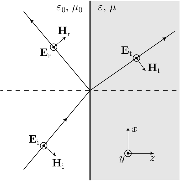
Figure 1: Schematic illustration of electric and magnetic fields for a TE-polarized mode at a planar vacuum–dielectric interface, for incident ($\mathbf{E}_{\mathrm{i}}$, $\mathbf{H}_{\mathrm{i}}$), reflected ($\mathbf{E}_{\mathrm{r}}$, $\mathbf{H}_{\mathrm{r}}$), and and transmitted ($\mathbf{E}_{\mathrm{t}}$, $\mathbf{H}_{\mathrm{t}}$) fields. For this polarization, the electric field is effectively scalar, while the magnetic-field polarization varies between media. This scalar-like behavior holds in any planar layered medium that varies in only one direction, such that $\epsilon(\mathbf{r})\equiv\epsilon(z)$ and $\mu(\mathbf{r})\equiv\mu(z)$.

In any TE-polarized plane-wave mode, the electric field is parallel to the interface. We take the polarization to be along the $y$-direction, such that $\mathbf{E}=\hat{y}E$, and thus $\mathbf{A}=\hat{y}A$. The Coulomb-gauge condition further implies $\partial_{y}{A}=0$, so that $(\nabla\times\mathbf{A})^{2}=|\nabla A_{y}|^{2}$. Then for any planar TE mode, the action (3) can be expressed in terms of the nonvanishing component of the vector potential $\phi(\mathbf{r},t):=A_{y}$ as

$$S_{\mathrm{\scriptscriptstyle TE}}=\frac{1}{2\mu_{0}}\int dt\int d\mathbf{r}\left[\frac{\epsilon_{\mathrm{r}}(z)}{c^{2}}\left(\partial_{t}\phi\right)^{2}-\frac{1}{\mu_{\mathrm{r}}(z)}|\nabla\phi|^{2}\right],$$ (6)

with corresponding wave equation

$$\nabla\cdot\frac{1}{\mu_{\mathrm{r}}({z})}\nabla\phi-\frac{\epsilon_{\mathrm{r}}({z})}{c^{2}}\partial_{t}^{2}\phi=0.$$ (7)

This action allows the TE-polarized modes to be represented explicitly in terms of a scalar field $\phi(\mathbf{r},t)$.

To treat the action for the transverse-magnetic (TM) polarization in a planar layered medium, it is convenient to introduce magnetic potentials $C_{0}$ and $\mathbf{C}$ Bordag, Kirsten, and Vassilevich (1999), in terms of which the fields are $\mathbf{H}=(\nabla C_{0}+\partial_{t}\mathbf{C})$ and $\mathbf{D}=(\nabla\times\mathbf{C})$. In terms of these potentials, the electromagnetic action is

$$S_{\mathrm{\scriptscriptstyle EM}}=\frac{1}{2\epsilon_{0}}\!\int\!dt\!\int\!d\mathbf{r}\left[\frac{\mu_{\mathrm{r}}(\mathbf{r})}{c^{2}}(\nabla C_{0}+\partial_{t}\mathbf{C})^{2}-\frac{(\nabla\times\mathbf{C})^{2}}{\epsilon_{\mathrm{r}}(\mathbf{r})}\right],$$ (8)

after changing the overall sign. Assuming the Coulomb-like gauge condition $\nabla\cdot\mu_{\mathrm{r}}\mathbf{C}=0$, the reduction to a scalar action for TM modes follows in the same way, with resulting action

$$S_{\mathrm{\scriptscriptstyle TM}}=\frac{1}{2\epsilon_{0}}\int dt\int d\mathbf{r}\left[\frac{\mu_{\mathrm{r}}(z)}{c^{2}}\left(\partial_{t}\psi\right)^{2}-\frac{1}{\epsilon_{\mathrm{r}}(z)}|\nabla\psi|^{2}\right],$$ (9)

and corresponding wave equation

$$\nabla\cdot\frac{1}{\epsilon_{\mathrm{r}}({z})}\nabla\psi-\frac{\mu_{\mathrm{r}}({z})}{c^{2}}\partial_{t}^{2}\psi=0,$$ (10)

where for any plane-wave mode $\psi(\mathbf{r},t)$ is the only nonvanishing component of $\mathbf{C}$. The TM scalar action and wave equation also follow simply from the TE case by noting that electromagnetism is invariant under the duality symmetry $\mathbf{E}\longleftrightarrow\mathbf{H}$, $\mathbf{B}\longleftrightarrow\mathbf{-D}$, and $\epsilon\longleftrightarrow\mu$.

The partition function for either scalar field is then a path integral over the fields in terms of the Euclidean action (i.e., with the replacement $t\rightarrow-i\hbar\beta$). For example, the TE path integral becomes

$$Z_{\mathrm{\scriptscriptstyle TE}}= \int D\phi\,\exp\left[-\frac{\epsilon_{0}c}{2\hbar}\int_{0}^{\beta\hbar c}d\tau\int d\mathbf{r}\,\right.$$

$$\left.\times\bigg{(}\epsilon_{\mathrm{r}}(\mathbf{r})|\partial_{\tau}\phi(\mathbf{r},\tau)|^{2}+\frac{1}{\mu_{\mathrm{r}}(\mathbf{r})}|\nabla\phi(\mathbf{r},\tau)|^{2}\bigg{)}\right],$$ (11)

where $\tau:=\beta\hbar c$. Changing to a scaled field variable

$$\tilde{\phi}(\mathbf{r},t):=\frac{\phi(\mathbf{r},t)}{\sqrt{\mu_{\mathrm{r}}(\mathbf{r})}}$$ (12)

removes explicit spatial dependence from the gradient term, but the change in integration measure to $D\tilde{\phi}$ introduces a functional determinant involving $\mu_{\mathrm{r}}$. This determinant ultimately drops out of the final calculation, provided we calculate only physically relevant differences between configurations amount to translations and rearrangements of the materials. Note also that subtleties involved in Faddeev–Popov-type gauge-fixing do not arise here, because the gauge condition used here is linear in the fields.

Then carrying out the Gaussian integration over the field variables, and performing the analogous procedure in the TM case, the partition functions become

$$\begin{array}[]{rcl}Z_{\mathrm{\scriptscriptstyle TE}}\!\!&=&\displaystyle\!\!\det\left[-\frac{1}{2}\epsilon_{\mathrm{r}}(\mathbf{r})\mu_{\mathrm{r}}(\mathbf{r})\partial_{\tau}^{2}-\frac{1}{2}\nabla^{2}-V_{\mathrm{\scriptscriptstyle TE}}(\mathbf{r})\right]^{-1/2}\\ Z_{\mathrm{\scriptscriptstyle TM}}\!\!&=&\displaystyle\!\!\det\left[-\frac{1}{2}\epsilon_{\mathrm{r}}(\mathbf{r})\mu_{\mathrm{r}}(\mathbf{r})\partial_{\tau}^{2}-\frac{1}{2}\nabla^{2}-V_{\mathrm{\scriptscriptstyle TM}}(\mathbf{r})\right]^{-1/2}\!\!,\end{array}$$ (13)

where the potentials are defined as

$$\begin{array}[]{rcl}V_{\mathrm{\scriptscriptstyle TE}}\!\!&:=&\displaystyle\!\!\frac{1}{2}\left[(\nabla\log\sqrt{\mu_{\mathrm{r}}})^{2}-\nabla^{2}\log\sqrt{\mu_{\mathrm{r}}}\right]\\ V_{\mathrm{\scriptscriptstyle TM}}\!\!&:=&\displaystyle\!\!\frac{1}{2}\left[(\nabla\log\sqrt{\epsilon_{\mathrm{r}}})^{2}-\nabla^{2}\log\sqrt{\epsilon_{\mathrm{r}}}\right]\end{array}$$ (14)

and these arise from the commutation of $\mu_{\mathrm{r}}(\mathbf{r})$ and $\epsilon_{\mathrm{r}}(\mathbf{r})$ through the derivative operators. Note that $V_{\mathrm{\scriptscriptstyle TE}}$ and $V_{\mathrm{\scriptscriptstyle TM}}$ will still appear in the path integral even without the field-rescaling procedure in Eq. (12). However, the development of the worldline path integrals is much more involved. Further details on this alternate derivation of the potentials will be provided elsewhere Mackrory, Bhattacharya, and Steck (tion), where we will also discuss their analytical and numerical evaluation at material interfaces.

III Worldline Path Integral

III.1 Casimir energies and renormalization

To extract zero-temperature Casimir energies from the partition function, we can compute the mean ground-state energy via $E=-\partial_{\beta}\log Z$. Since the divergent absolute energy is not a physical observable, it is important to renormalize the energy. That is, one should subtract the energy of a reference configuration to obtain a finite interaction energy: $E=-\partial_{\beta}(\log Z-\log Z_{0})$. The reference configuration depends on the geometry of interest, but a typical choice is an arbitrarily large separation of the material objects.

The derivation of the worldline path integral then proceeds by evaluating the partition-function determinants (13) via the identity

$$\log\det[A]=\mathrm{tr}\log[A],$$ (15)

and then using the integral representation

$$\log[A]-\log[B]=\int_{0}^{\infty}\!\frac{d\mathcal{T}}{\mathcal{T}}\Big{(}e^{-B\mathcal{T}}-e^{-A\mathcal{T}}\Big{)}$$ (16)

for the logarithm. Note that without the renormalizing subtraction here, the integral diverges at the lower limit—this is the same ultraviolet divergence that comes from computing Casimir energies via mode-summation. For simplicity of notation, we will normally not write out the subtraction of the reference configuration, so the divergent expressions that follow must be interpreted as representing the finite quantity that remains after this subtraction. From Eq. (13), the (non-renormalized) mean energy is

$$E_{\mathrm{\scriptscriptstyle TE}}=-\frac{\partial_{\beta}}{2}\!\!\int_{0}^{\infty}\!\!\frac{d\mathcal{T}}{\mathcal{T}}\,\mathrm{tr}\,e^{\mathcal{T}\left[(1/2)\epsilon_{\mathrm{r}}(\hat{\mathbf{x}})\mu_{\mathrm{r}}(\hat{\mathbf{x}})\partial_{\tau}^{2}+(1/2)\nabla^{2}+V_{\mathrm{\scriptscriptstyle TE}}(\hat{\mathbf{x}})\right]},$$ (17)

where now the notation $\hat{\mathbf{x}}$ emphasizes the operator nature of the field variable. We can evaluate the trace for this operator by introducing an auxiliary Hilbert space with $\langle\mathbf{x},\tau|\hat{\mathbf{x}}|\psi\rangle=\mathbf{x}\psi(\mathbf{x},\tau)$, $\langle\mathbf{x},\tau|\hat{\mathbf{p}}|\psi\rangle=-i\nabla\psi(\mathbf{x},\tau)$, $\langle\mathbf{x},\tau|\hat{\tau}|\psi\rangle=\tau\psi(\mathbf{x},\tau)$, $\langle\mathbf{x},\tau|\hat{p}_{\tau}|\psi\rangle=-i\partial_{\tau}\psi(\mathbf{x},\tau),$ and $\langle\mathbf{x}|\mathbf{p}\rangle=e^{i\mathbf{x}\cdot\mathbf{p}}$. Then expressing the trace as a spacetime integration, the result is

$$E_{\mathrm{\scriptscriptstyle TE}} =-\frac{\partial_{\beta}}{2}\int_{0}^{\infty}\!\!\frac{d\mathcal{T}}{\mathcal{T}}\,\int_{0}^{\beta\hbar c}\!\!\!d\tau_{0}\int d\mathbf{x}_{0}$$

$$\times\langle\mathbf{x}_{0},\tau_{0}|e^{-\left(\epsilon_{\mathrm{r}}(\hat{\mathbf{x}})\mu_{\mathrm{r}}(\hat{\mathbf{x}})\hat{p}_{\tau}^{2}/2+\hat{\mathbf{p}}^{2}/2+V_{\mathrm{\scriptscriptstyle TE}}(\hat{\mathbf{x}})\right)\mathcal{T}}|\mathbf{x}_{0},\tau_{0}\rangle.$$ (18)

Since the matrix element is independent of $\hat{\tau}$, it is only necessary to develop the path integral in the spatial dimensions. Splitting the exponential operator into $N$ pieces, and inserting spatial position and momentum identities $1=\int d\mathbf{x}_{j}\,|\mathbf{x}_{j}\rangle\langle\mathbf{x}_{j}|=(2\pi)^{-(D-1)}\int d\mathbf{p}_{j}\,|\mathbf{p}_{j}\rangle\langle\mathbf{p}_{j}|$ between each piece, the matrix element becomes

$$\langle\mathbf{x}_{0},\tau_{0}|e^{-\left[\epsilon_{\mathrm{r}}(\hat{\mathbf{x}})\mu_{\mathrm{r}}(\hat{\mathbf{x}})\hat{p}_{\tau}^{2}/2+\hat{\mathbf{p}}^{2}/2+V_{\mathrm{\scriptscriptstyle TE}}(\hat{\mathbf{x}})\right]\mathcal{T}}|\mathbf{x}_{0},\tau_{0}\rangle$$

$$\hskip 5.69054pt= \int\prod_{j=1}^{N}\left(\frac{d\mathbf{x}_{j}d\mathbf{p}_{j}}{(2\pi)^{D-1}}\right)\bigg{\{}\delta^{D-1}(\mathbf{x}_{N}-\mathbf{x}_{0})\prod_{k=0}^{N}\big{[}\langle\mathbf{x}_{k}|\mathbf{p}_{k}\rangle$$

$$\times\langle\mathbf{p}_{k}|e^{-\left(\epsilon_{\mathrm{r}}(\hat{\mathbf{x}})\mu_{\mathrm{r}}(\hat{\mathbf{x}})\hat{p}_{\tau}^{2}/2+\hat{\mathbf{p}}^{2}/2+V_{\mathrm{\scriptscriptstyle TE}}(\hat{\mathbf{x}})\right)\Delta\mathcal{T}}|\mathbf{x}_{k-1}\rangle\big{]}\bigg{\}},$$ (19)

where $D$ is the spacetime dimension, $\Delta\mathcal{T}=\mathcal{T}/N$, and the path-closure condition $\mathbf{x}_{N}=\mathbf{x}_{0}$ from the trace is now enforced by the delta function. Replacing operators by eigenvalues, using $\langle\mathbf{x}_{j}|\mathbf{p}_{j}\rangle=e^{i\mathbf{p}_{j}\cdot\mathbf{x}_{j}}$, and evaluating the momentum integrals leaves

$$\langle\mathbf{x}_{0},\tau_{0}|e^{-\left[\epsilon_{\mathrm{r}}(\hat{\mathbf{x}})\mu_{\mathrm{r}}(\hat{\mathbf{x}})\hat{p}_{\tau}^{2}/2+\hat{\mathbf{p}}^{2}/2+V_{\mathrm{\scriptscriptstyle TE}}(\hat{\mathbf{x}})\right]\mathcal{T}}|\mathbf{x}_{0},\tau_{0}\rangle$$

$$\hskip 5.69054pt= \int\prod_{j=1}^{N}\frac{d\mathbf{x}_{j}}{(2\pi\Delta\mathcal{T})^{(D-1)/2}}\bigg{\{}\delta^{D-1}(\mathbf{x}_{N}-\mathbf{x}_{0})$$

$$\times\prod_{k=1}^{N}\left[e^{-(\mathbf{x}_{k}-\mathbf{x}_{k-1})^{2}/(2\Delta\mathcal{T})-\Delta\mathcal{T}V_{\mathrm{\scriptscriptstyle TE}}(\mathbf{x}_{k-1})}\right.$$

$$\left.\times\,e^{-\epsilon_{\mathrm{r}}(\mathbf{x}_{k-1})\,\mu_{\mathrm{r}}(\mathbf{x}_{k-1})\,\hat{p}_{\tau}^{2}\Delta\mathcal{T}/2}\right]\bigg{\}}.$$ (20)

Putting this back into Eq. (18) and carrying out the remaining integrals over $\tau_{0}$ and $p_{\tau}$ gives

$$E_{\mathrm{\scriptscriptstyle TE}}= -\frac{\hbar c}{2}\int_{0}^{\infty}\!\!\frac{d\mathcal{T}}{\mathcal{T}}\int\prod_{j=1}^{N}\frac{d\mathbf{x}_{j}}{(2\pi\Delta\mathcal{T})^{(D-1)/2}}$$

$$\times\frac{\delta^{D-1}(\mathbf{x}_{N}-\mathbf{x}_{0})}{[2\pi\mathcal{T}N^{-1}\sum_{\ell=0}^{N-1}\epsilon_{\mathrm{r}}(\mathbf{x}_{\ell})\,\mu_{\mathrm{r}}(\mathbf{x}_{\ell})]^{1/2}}$$

$$\times\prod_{k=1}^{N}\left[e^{-(\mathbf{x}_{k}-\mathbf{x}_{k-1})^{2}/(2\Delta\mathcal{T})-\Delta\mathcal{T}V_{\mathrm{\scriptscriptstyle TE}}(\mathbf{x}_{k-1})}\right].$$ (21)

This expression already exhibits the form of the numerical method: The Gaussian densities, in conjunction with the delta function, define a probability measure for paths (random walks) that begin and end at $\mathbf{x}_{0}$. The contribution of the material body enters in the evaluation of $[\epsilon_{\mathrm{r}}(\mathbf{r})\,\mu_{\mathrm{r}}(\mathbf{r})]$ and $V_{\mathrm{\scriptscriptstyle TE}}(\mathbf{r})$ [or $V_{\mathrm{\scriptscriptstyle TM}}(\mathbf{r})$ in the TM case] along the path.

The presence of the delta function $\delta(\mathbf{x}_{N}-\mathbf{x}_{0})$ leads to an additional overall normalization constant $(2\pi\mathcal{T})^{-(D-1)/2}$, if the sum encompasses only paths that close, such that $\mathbf{x}_{N}=\mathbf{x}_{0}$. This follows from the expression Hörmander (1983)

$$\int d\mathbf{q}\,\delta[h(\mathbf{q})]\,f(\mathbf{q})=\int_{h^{-1}(0)}\!\!\!\!\!dS\,\frac{1}{|\nabla h(\mathbf{q})|}f(\mathbf{q}),$$ (22)

where $S$ is the surface satisfying $h(\mathbf{q})=0$, and

$$|\nabla h(\mathbf{q})|=\sqrt{\sum_{k}\left(\frac{\partial h}{\partial q_{k}}\right)^{2}}$$ (23)

is the Euclidean norm of the gradient vector. In the case at hand, the delta function restricts a sum of $N$ Gaussian integrals to have a total of zero. Defining the increments $\Delta\mathbf{x}_{n}:=\mathbf{x}_{n+1}-\mathbf{x}_{n}$, the path-closure constraint is $\smash{\delta(\sum_{k=0}^{N-1}\Delta\mathbf{x}_{k})}$. Accounting for the remaining normalization constant of the Gaussian $\mathbf{x}_{N}$ integral (as part of $dS$), the extra contribution for considering only closed paths ($\mathbf{x}_{N}=\mathbf{x}_{0}$) in the path integral is $(2\pi\Delta\mathcal{T}N)^{-(D-1)/2}=(2\pi\mathcal{T})^{-(D-1)/2}$.

Taking the remaining $N-1$ Gaussian factors to be the probability measure for the paths, in a Monte-Carlo interpretation of the path integrals, the sample paths are Brownian bridges Karatzas and Shreve (1991) in the limit of large $N$. To be more precise, a Wiener path $W(t)$ is a continuous time random walk, where each increment has ensemble average $\langle\!\langle dW(t)\rangle\!\rangle=0$ (where the double brackets denote an ensemble average) and variance $\langle\!\langle dW^{2}(t)\rangle\!\rangle=dt$, with $\langle\!\langle dW(t)\,dW(t^{\prime})\rangle\!\rangle=0$ for $t\neq t^{\prime}$. A Brownian bridge $B_{\mathcal{T}}(t)$ is a Wiener path subject to the pinning condition $B_{\mathcal{T}}(\mathcal{T})=0$. (The bridges may also be defined such that they are pinned to other endpoints.) Brownian bridges thus form a subset of zero measure of all possible Wiener paths.

The (unrenormalized) Casimir energy can then be rewritten in continuous-time notation as

$$E_{\mathrm{\scriptscriptstyle TE}}=-\frac{\hbar c}{2(2\pi)^{D/2}}\int_{0}^{\infty}\!\!\!\frac{d\mathcal{T}}{\mathcal{T}^{1+D/2}}\int\!d\mathbf{x}_{0}\,{\Bigg{\langle}\kern-3.50006pt\Bigg{\langle}}\frac{e^{-\mathcal{T}\langle V_{\mathrm{\scriptscriptstyle TE}}\rangle}}{\langle\epsilon_{\mathrm{r}}\mu_{\mathrm{r}}\rangle^{1/2}}{\Bigg{\rangle}\kern-3.50006pt\Bigg{\rangle}}_{\!\!\mathbf{x}(t)}$$ (24)

for the TE polarization, and

$$E_{\mathrm{\scriptscriptstyle TM}}=-\frac{\hbar c}{2(2\pi)^{D/2}}\int_{0}^{\infty}\!\!\!\frac{d\mathcal{T}}{\mathcal{T}^{1+D/2}}\int\!d\mathbf{x}_{0}\,{\Bigg{\langle}\kern-3.50006pt\Bigg{\langle}}\frac{e^{-\mathcal{T}\langle V_{\mathrm{\scriptscriptstyle TM}}\rangle}}{\langle\epsilon_{\mathrm{r}}\mu_{\mathrm{r}}\rangle^{1/2}}{\Bigg{\rangle}\kern-3.50006pt\Bigg{\rangle}}_{\!\!\mathbf{x}(t)}$$ (25)

for the TM polarization, where only the coordinate $\mathbf{x}_{0}$ is elided in the notation $\smash{\langle\!\langle\cdots\rangle\!\rangle_{\mathbf{x}(t)}}$ that denotes an ensemble average over vector Brownian bridges $\mathbf{x}(t)$ starting and returning to $\mathbf{x}_{0}$, and

$$\langle f\rangle:=\frac{1}{\mathcal{T}}\int_{0}^{\mathcal{T}}\!\!dt\,f[\mathbf{x}(t)]=\frac{1}{N}\sum_{k=0}^{N-1}f(\mathbf{x}_{k})$$ (26)

is a shorthand for the average value of $f(\mathbf{r})$, evaluated along the path. In this paper, we will stick to the evaluation of the TE path integral (24) in the presence of dielectric-only materials, which simplifies to

$$E_{\mathrm{\scriptscriptstyle TE}}=-\frac{\hbar c}{2(2\pi)^{D/2}}\int_{0}^{\infty}\!\!\!\frac{d\mathcal{T}}{\mathcal{T}^{1+D/2}}\int\!d\mathbf{x}_{0}\,{\Big{\langle}\kern-3.50006pt\Big{\langle}}\langle\epsilon_{\mathrm{r}}\rangle^{-1/2}{\Big{\rangle}\kern-3.50006pt\Big{\rangle}}_{\!\!\mathbf{x}(t)}.$$ (27)

Note that this has the same form as the TM path integral (25) in the presence of magnetic-only materials.

III.2 Casimir–Polder energies

In principle, Eqs. (24) and (25) can yield Casimir–Polder energies for an atom interacting with a macroscopic body by treating the atom as a small chunk of magnetodielectric material. However, this is numerically inefficient: the vast majority of paths will not intersect the atom, and will thus not contribute to the renormalized potential. (Note that only paths that intersect both bodies will contribute to the properly renormalized, two-body Casimir energy.) It is therefore useful to develop specialized path integrals for evaluating Casimir–Polder potentials.

To introduce the atom, we may regard it as producing localized perturbations $\delta\epsilon_{\mathrm{r}}(\mathbf{r})$ and $\delta\mu_{\mathrm{r}}(\mathbf{r})$ to the background relative permittivity and permeability, respectively. In the dipole approximation, these perturbations are given explicitly in terms of delta functions as

$$\begin{array}[]{rcl}\delta\epsilon_{\mathrm{r}}(\mathbf{r})\!\!&=&\!\!\displaystyle\frac{\alpha_{0}}{\epsilon_{0}}\delta^{D-1}(\mathbf{r}-\mathbf{r}_{\mathrm{\scriptscriptstyle A}})\\ \delta\mu_{\mathrm{r}}(\mathbf{r})\!\!&=&\!\!\displaystyle\beta_{0}\mu_{0}\,\delta^{D-1}(\mathbf{r}-\mathbf{r}_{\mathrm{\scriptscriptstyle A}}),\end{array}$$ (28)

where $\alpha_{0}$ and $\beta_{0}$ are respectively the static polarizability and magnetizability of the atom, and $\mathbf{r}_{\mathrm{\scriptscriptstyle A}}$ is the location of the atom. [Note that the polarizability and magnetizability are defined such that the electric and magnetic induced dipole moments are $\mathbf{d}=\alpha_{0}\mathbf{E}$ and $\mathbf{m}=\beta_{0}\mu_{0}\mathbf{H}$, while the polarization and magnetization are conventionally given in terms of the perturbations by $\mathbf{P}=\delta\epsilon\,\mathbf{E}$ and $\mathbf{M}=(\delta\mu/\mu_{0})\,\mathbf{H}$.] The relevant energy is then the difference between the Casimir energies with and without the perturbations. To first order in the perturbations,

$$\begin{array}[]{rcl}\delta E[\epsilon_{\mathrm{r}},\mu_{\mathrm{r}}]\!\!&=&\!\!\displaystyle E[\epsilon_{\mathrm{r}}+\delta\epsilon_{\mathrm{r}},\mu_{\mathrm{r}}+\delta\mu_{\mathrm{r}}]-E[\epsilon_{\mathrm{r}},\mu_{\mathrm{r}}]\\ \!\!&=&\!\!\displaystyle\int d\mathbf{r}\left[\frac{\delta E}{\delta\epsilon_{\mathrm{r}}}\,\delta\epsilon_{\mathrm{r}}(\mathbf{r})+\frac{\delta E}{\delta\mu_{\mathrm{r}}}\,\delta\mu_{\mathrm{r}}(\mathbf{r})\right].\end{array}$$ (29)

Then putting in the perturbations (28), we identify this energy as the Casimir–Polder potential,

$$V_{\mathrm{\scriptscriptstyle CP}}(\mathbf{r}_{\mathrm{\scriptscriptstyle A}})=\frac{\alpha_{0}}{\epsilon_{0}}\left(\frac{\delta E}{\delta\epsilon_{\mathrm{r}}(\mathbf{r}_{\mathrm{\scriptscriptstyle A}})}\right)+\beta_{0}\mu_{0}\left(\frac{\delta E}{\delta\mu_{\mathrm{r}}(\mathbf{r}_{\mathrm{\scriptscriptstyle A}})}\right),$$ (30)

written here in terms of functional derivatives of the Casimir energy evaluated at the atomic position. Note that in treating the atom as arbitrarily well-localized, the perturbations (28) are technically divergent. However, the effect of the perturbations is still small, so the expansion here is really in terms of $\alpha_{0}$ and $\beta_{0}$ (i.e., this is a shorthand for taking a small but finite radius of the atom to zero at the end of the calculation). Note also that the expression (30) is invariant under the duality transformation $\epsilon_{\mathrm{r}}\longleftrightarrow\mu_{\mathrm{r}}$, $\alpha_{0}/\epsilon_{0}\longleftrightarrow\beta_{0}\mu_{0}$ Buhmann and Scheel (2009); Safari et al. (2008).

Then to carry out the explicit expansion in Eq. (29) to compute the functional derivatives in the Casimir–Polder potential (30), we need the path-average expansion

$$\begin{array}[]{l}\displaystyle\big{\langle}(\epsilon_{\mathrm{r}}+\delta\epsilon_{\mathrm{r}})(\mu_{\mathrm{r}}+\delta\mu_{\mathrm{r}})\big{\rangle}^{-1/2}\\ \displaystyle\hskip 42.67912pt=\frac{1}{\langle\epsilon_{\mathrm{r}}\mu_{\mathrm{r}}\rangle^{1/2}}-\frac{\langle\delta\epsilon_{\mathrm{r}}\,\mu_{r}\rangle}{2\langle\epsilon_{\mathrm{r}}\mu_{\mathrm{r}}\rangle^{3/2}}-\frac{\langle\epsilon_{\mathrm{r}}\,\delta\mu_{\mathrm{r}}\rangle}{2\langle\epsilon_{\mathrm{r}}\mu_{\mathrm{r}}\rangle^{3/2}},\end{array}$$ (31)

as well as the expansions of the potentials (14), which are necessary to include the contributions of the potential factors of the form $e^{-\mathcal{T}\langle V_{\mathrm{\scriptscriptstyle TE}}\rangle}$:

$$\begin{array}[]{l}V_{\mathrm{\scriptscriptstyle TE}}\big{[}\mu_{\mathrm{r}}+\delta\mu_{\mathrm{r}}\big{]}\\ \hskip 14.22636pt=\displaystyle\frac{1}{8}\big{[}\nabla\log(\mu_{\mathrm{r}}+\delta\mu_{\mathrm{r}})\big{]}^{2}-\frac{1}{4}\nabla^{2}\log(\mu_{\mathrm{r}}+\delta\mu_{\mathrm{r}})\\ \\ \hskip 14.22636pt=\displaystyle V_{\mathrm{\scriptscriptstyle TE}}[\mu_{\mathrm{r}}]+\frac{1}{4}\left[\left(\nabla\frac{\delta\mu_{\mathrm{r}}}{\mu_{\mathrm{r}}}\right)\cdot\nabla\log\mu_{\mathrm{r}}-\nabla^{2}\frac{\delta\mu_{\mathrm{r}}}{\mu_{\mathrm{r}}}\right].\end{array}$$ (32)

These expressions serve to expand Eqs. (24) and (25), integrating by parts where necessary. Integrating over the starting (and ending) point $\mathbf{x}_{0}$ of all rigid translations of a particular path and computing the path average gives

$$\int d\mathbf{x}_{0}\,\big{\langle}f(\mathbf{x})\,\delta^{D-1}(\mathbf{x}-\mathbf{r}_{\mathrm{\scriptscriptstyle A}})\big{\rangle}=f(\mathbf{r}_{\mathrm{\scriptscriptstyle A}}),$$ (33)

where, after removing the delta function, the resulting “paths” are averages over all rigid translations of the same path such that the path intersects $\mathbf{r}_{\mathrm{\scriptscriptstyle A}}$. The ensemble average of paths is equivalently sampled by simply averaging over paths beginning and ending at $\mathbf{r}_{\mathrm{\scriptscriptstyle A}}$. Assembling these pieces gives the following expression for the TE-polarization Casimir–Polder potential:

$$\begin{array}[]{l}\displaystyle V_{\mathrm{\scriptscriptstyle CP}}^{\mathrm{\scriptscriptstyle(TE)}}(\mathbf{r}_{\mathrm{\scriptscriptstyle A}})\\ \displaystyle\hskip 8.53581pt=\frac{\hbar c}{4(2\pi)^{D/2}}\int_{0}^{\infty}\!\!\frac{d\mathcal{T}}{\mathcal{T}^{1+D/2}}\\ \displaystyle\hskip 22.76219pt{}\times{\Bigg{\langle}\kern-3.50006pt\Bigg{\langle}}\left(\frac{\alpha_{0}\mu_{\mathrm{r}}(\mathbf{r}_{\mathrm{\scriptscriptstyle A}})}{\epsilon_{0}}+\beta_{0}\mu_{0}\epsilon_{\mathrm{r}}(\mathbf{r}_{\mathrm{\scriptscriptstyle A}})\right)\frac{e^{-\mathcal{T}\langle V_{\mathrm{\scriptscriptstyle TE}}\rangle}}{\langle\epsilon_{\mathrm{r}}\mu_{\mathrm{r}}\rangle^{3/2}}\\ \displaystyle\hskip 45.5244pt-\frac{\beta_{0}\mu_{0}\mathcal{T}}{2\mu_{\mathrm{r}}(\mathbf{r}_{\mathrm{\scriptscriptstyle A}})}\Big{[}\nabla^{2}(\log\mu_{\mathrm{r}})+\nabla(\log\mu_{\mathrm{r}})\cdot\nabla+\nabla^{2}\Big{]}\\ \displaystyle\hskip 93.89409pt\times\frac{e^{-\mathcal{T}\langle V_{\mathrm{\scriptscriptstyle TE}}\rangle}}{\langle\epsilon_{\mathrm{r}}\mu_{\mathrm{r}}\rangle^{1/2}}{\Bigg{\rangle}\kern-3.50006pt\Bigg{\rangle}}_{\mathbf{x}(t),\,\mathbf{x}(0)=\mathbf{x}(\mathcal{T})=\mathbf{r}_{\mathrm{\scriptscriptstyle A}}}.\end{array}$$ (34)

For TM polarization, the corresponding expression is

$$\begin{array}[]{l}\displaystyle V_{\mathrm{\scriptscriptstyle CP}}^{\mathrm{\scriptscriptstyle(TM)}}(\mathbf{r}_{\mathrm{\scriptscriptstyle A}})\\ \displaystyle\hskip 8.53581pt=\frac{\hbar c}{4(2\pi)^{D/2}}\int_{0}^{\infty}\!\!\frac{d\mathcal{T}}{\mathcal{T}^{1+D/2}}\\ \displaystyle\hskip 22.76219pt{}\times{\Bigg{\langle}\kern-3.50006pt\Bigg{\langle}}\left(\beta_{0}\mu_{0}\epsilon_{\mathrm{r}}(\mathbf{r}_{\mathrm{\scriptscriptstyle A}})+\frac{\alpha_{0}\mu_{\mathrm{r}}(\mathbf{r}_{\mathrm{\scriptscriptstyle A}})}{\epsilon_{0}}\right)\frac{e^{-\mathcal{T}\langle V_{\mathrm{\scriptscriptstyle TM}}\rangle}}{\langle\epsilon_{\mathrm{r}}\mu_{\mathrm{r}}\rangle^{3/2}}\\ \displaystyle\hskip 45.5244pt-\frac{\alpha_{0}\mathcal{T}}{2\epsilon_{0}\epsilon_{\mathrm{r}}(\mathbf{r}_{\mathrm{\scriptscriptstyle A}})}\Big{[}\nabla^{2}(\log\epsilon_{\mathrm{r}})+\nabla(\log\epsilon_{\mathrm{r}})\cdot\nabla+\nabla^{2}\Big{]}\\ \displaystyle\hskip 93.89409pt\times\frac{e^{-\mathcal{T}\langle V_{\mathrm{\scriptscriptstyle TM}}\rangle}}{\langle\epsilon_{\mathrm{r}}\mu_{\mathrm{r}}\rangle^{1/2}}{\Bigg{\rangle}\kern-3.50006pt\Bigg{\rangle}}_{\mathbf{x}(t),\,\mathbf{x}(0)=\mathbf{x}(\mathcal{T})=\mathbf{r}_{\mathrm{\scriptscriptstyle A}}}.\end{array}$$ (35)

In this paper we will evaluate the TE path integral for an electric-dipole atom coupled to a dielectric-only material, in which case the path integral (34) simplifies considerably to

$$V_{\mathrm{\scriptscriptstyle CP}}^{\mathrm{\scriptscriptstyle(TE)}}(\mathbf{r}_{\mathrm{\scriptscriptstyle A}})=\frac{\hbar c\alpha_{0}}{4(2\pi)^{D/2}\epsilon_{0}}\int_{0}^{\infty}\!\!\frac{d\mathcal{T}}{\mathcal{T}^{1+D/2}}\,{\Big{\langle}\kern-3.50006pt\Big{\langle}}\langle\epsilon_{\mathrm{r}}\rangle^{-3/2}{\Big{\rangle}\kern-3.50006pt\Big{\rangle}}_{\mathbf{x}(t)},$$ (36)

which has the same form as the TM path integral for a magnetic-dipole atom coupled to a magnetic-only material. The TM path integral also simplifies somewhat in this case, but still involves the potential $V_{\mathrm{\scriptscriptstyle TM}}$ in Eqs. (14), the evaluation of which we will consider in the future Mackrory, Bhattacharya, and Steck (tion).

IV Analytic Worldline Summation

To further investigate the worldline path integrals, we will consider their analytic evaluation and show that the dielectric-body path integrals (27) and (36) converge to known solutions in planar geometries. In certain limits, this evaluation is quite straightforward. For example, for a polarizable atom interacting with a perfectly conducting planar surface (corresponding to $\epsilon_{\mathrm{r}}\longrightarrow\infty$), the conductor imposes Dirichlet boundary conditions on the scalar field, as in previous work on Casimir worldlines with background potentials Gies, Langfeld, and Moyaerts (2003). In the renormalized form of the path integral (36), the integrand $\langle\epsilon_{\mathrm{r}}\rangle^{-3/2}-1$ is averaged over the ensemble. The integrand vanishes for paths that do not touch the surface, but takes the value $-1$ for those that do. Thus, the ensemble average yields the probability for a Brownian bridge to cross the surface, with an overall minus sign. For a Brownian bridge $B_{\mathcal{T}}(t)$, the probability to cross a boundary at distance $d$ is well-known, and takes the value

$$P_{\mathrm{cross}}=\exp(-2d^{2}/\mathcal{T}).$$ (37)

Putting this value into the path integral and carrying out the remaining integral gives

$$V_{\mathrm{\scriptscriptstyle CP}}^{\mathrm{\scriptscriptstyle(TE)}}(\mathbf{r}_{\mathrm{\scriptscriptstyle A}})=-\frac{\hbar c\alpha_{0}}{64\pi^{2}\epsilon_{0}d^{4}}$$ (38)

for $D=4$, which is the correct contribution of the TE polarization to the Casimir–Polder potential in this limit.

In the case of a more general planar dielectric surface, the relevant statistic to describe the path average $\langle\epsilon_{\mathrm{r}}\rangle$ is the sojourn-time functional (see Appendix B)

$$T_{\mathrm{s}}[B_{\mathcal{T}}(t);d]:=\int_{0}^{1}\!dt\,\Theta[B_{\mathcal{T}}(t)-d],$$ (39)

which is the time a Brownian bridge $B_{\mathcal{T}}(t)$ spends past a boundary at distance $d$ (here $\Theta(x)$ is the Heaviside function). The probability distribution for $T_{\mathrm{s}}$ is known exactly for a Brownian bridge Takács (1999); Hooghiemstra (2002), and the probability density may be written

$$\begin{array}[]{rcl}\displaystyle f_{T_{\mathrm{s}}}(x)\!\!&=&\!\!\displaystyle\left[1-e^{-2d^{2}/\mathcal{T}}\right]\delta(x-0^{+})\\ &&\displaystyle{}+\sqrt{\frac{8d^{2}(\mathcal{T}-x)}{\pi x\mathcal{T}^{3}}}\,e^{-2d^{2}/(\mathcal{T}-x)}\\ &&\displaystyle{}+\left(1-\frac{4d^{2}}{\mathcal{T}}\right)\frac{e^{-2d^{2}/\mathcal{T}}}{\mathcal{T}}\,\mathrm{erfc}\left(\sqrt{\frac{2d^{2}x}{\mathcal{T}(\mathcal{T}-x)}}\right).\end{array}$$ (40)

This may be used to compute the ensemble average of $\langle\epsilon_{\mathrm{r}}\rangle^{-3/2}-1=(1+\chi T_{\mathrm{s}})^{-3/2}-1$, where $\chi=\epsilon_{\mathrm{r}}-1$ is the dielectric susceptibility, in the renormalized form of the path integral (36) which then yields the TE Casimir–Polder potential for arbitrary $\chi$. However, we will defer this solution in favor of deriving it via a slightly different method.

IV.1 Iterated Laplace transform

The derivation of the sojourn-time density (40) involves the solution to a diffusion equation to obtain an iterated Laplace transform of the density. Inverting the Laplace transforms then gives the density directly Hooghiemstra (2002). A modification of this procedure provides the same solution for the Casimir–Polder potential for a polarizable atom and a planar dielectric half-space without directly knowing the sojourn-time density. This method then extends to other situations where the density for the relevant path statistic has a cumbersome form (such as the Casimir energy or Casimir–Polder potential for two parallel, planar dielectric interfaces) or is not readily available in closed form (such as the Casimir energies for the TM polarization for planar dielectric interfaces).

The method employs the Feynman-Kac formula Durrett (1996); Karatzas and Shreve (1991), which states that a solution $f(x,t)$ to the diffusion equation

$$\partial_{t}f=\frac{1}{2}\partial_{x}^{2}f-[V(x)+\lambda]f+g(x),$$ (41)

with particle killing rate $V(x)$ and source function $g(x)$, can also be written as an ensemble average over diffusive trajectories,

$$f(x,t)= \,{\bigg{\langle}\kern-3.50006pt\bigg{\langle}}f_{0}[x+W(t)]\,e^{-\lambda t-\int_{0}^{t}\!dt^{\prime}\,V[x+W(t^{\prime})]}$$

$$+\int_{0}^{t}\!dt^{\prime}\,g[x+W(t^{\prime})]\,e^{-\lambda t^{\prime}-\int_{0}^{t^{\prime}}\!dt^{\prime\prime}\,V[x+W(t^{\prime\prime})]}{\bigg{\rangle}\kern-3.50006pt\bigg{\rangle}},$$ (42)

where the initial condition is $f_{0}(x)=f(x,t=0)$, and $\langle\!\langle\cdots\rangle\!\rangle$ denotes the ensemble average over Wiener processes $W(t)$ (with initial condition $W(0)=0$, increment means $\langle\!\langle dW(t)\rangle\!\rangle=0$ and increment variance $\langle\!\langle dW(t)^{2}\rangle\!\rangle=dt$). The formula in one dimension is sufficient for Casimir calculations with planar geometries, but the method here readily generalizes to multiple dimensions.

In steady state, the solution is independent of the initial condition, and choosing the source function to be $g(x,t)=\delta(x)$, the path average becomes

$$f(x)=\int_{0}^{\infty}\!\!dt^{\prime}\,{\bigg{\langle}\kern-3.50006pt\bigg{\langle}}\delta[x+W(t^{\prime})]\,e^{-\lambda t^{\prime}-\int_{0}^{t^{\prime}}\!dt^{\prime\prime}\,V[x(t^{\prime\prime})]}{\bigg{\rangle}\kern-3.50006pt\bigg{\rangle}},$$ (43)

where $f(x)$ satisfies the eigenvalue equation

$$\lambda f=\frac{1}{2}\partial_{x}^{2}f-V(x)\,f+\delta(x).$$ (44)

The delta function pins the paths at the end point such that $W(t)=-x$. In the worldline path integrals, solutions with closed paths are then obtained by setting $x=0$ in the solution $f(x)$. The further restriction to Brownian-bridge sample paths requires a further normalization factor of $\smash{(2\pi\mathcal{T})^{-1/2}}$, which follows from Eqs. (22) and (23).

The worldline path integrals (27) and (36) for the Casimir and Casimir–Polder energies both have the general form

$$U({x}_{0})=\int_{0}^{\infty}\!\!\frac{d\mathcal{T}}{\mathcal{T}^{1+D/2}}\,{\bigg{\langle}\kern-3.50006pt\bigg{\langle}}\frac{1}{\langle\epsilon_{\mathrm{r}}\rangle^{\alpha}}{\bigg{\rangle}\kern-3.50006pt\bigg{\rangle}}_{\!{x}(t)},$$ (45)

where $\alpha=1/2$ for Casimir energies and $\alpha=3/2$ for Casimir–Polder energies, and the paths $x(t)$ satisfy $x(0)=x(\mathcal{T})=x_{0}$. Then the identity

$$\frac{1}{[h({x})]^{\alpha}}=\frac{1}{\Gamma(\alpha)}\int_{0}^{\infty}\!\!ds\,s^{\alpha-1}e^{-s\,h({x})},$$ (46)

where $\Gamma[\alpha]$ is the gamma function, allows us to exponentiate the material dependence in Eq. (45):

$$U(x_{0})= \,\frac{1}{\Gamma(\alpha)}\int_{0}^{\infty}\!\!\frac{d\mathcal{T}}{\mathcal{T}^{1+(D-1)/2-\alpha}}\int_{0}^{\infty}\!\!ds\,s^{\alpha-1}$$

$$\hskip 42.67912pt{}\times{\bigg{\langle}\kern-3.50006pt\bigg{\langle}}\frac{1}{\sqrt{\mathcal{T}}}\,e^{-s\int_{0}^{\mathcal{T}}dt\,\epsilon_{\mathrm{r}}[x(t)]}{\bigg{\rangle}\kern-3.50006pt\bigg{\rangle}}_{\!{x}(t)}.$$ (47)

The $\mathcal{T}$ integral here has the form of a Mellin transform which can be related to a Laplace transform via an integration of the form Lew (1975)

$$\int_{0}^{\infty}\!\!d\mathcal{T}\,\mathcal{T}^{z-1}\,f(\mathcal{T})$$

$${}\hskip 14.22636pt=\frac{1}{\Gamma(1-z)}\int_{0}^{\infty}\!\!d\lambda\,\lambda^{-z}\int_{0}^{\infty}\!\!d\mathcal{T}\,e^{-\lambda\mathcal{T}}f(\mathcal{T}).$$ (48)

Thus, the factor $\mathcal{T}^{-1-(D-1)/2+\alpha}$ may be recast as an additional integral:

$$U(x_{0})= \int_{0}^{\infty}\!\!d\lambda\,\frac{\lambda^{(D-1)/2-\alpha}}{\Gamma[(D-1)/2-\alpha]}\int_{0}^{\infty}\!\!ds\,\frac{s^{\alpha-1}}{\Gamma(\alpha)}$$

$$\hskip 8.53581pt{}\times\int_{0}^{\infty}\!\!d\mathcal{T}\,{\bigg{\langle}\kern-3.50006pt\bigg{\langle}}\frac{1}{\sqrt{\mathcal{T}}}\,e^{-\lambda\mathcal{T}-s\int_{0}^{\mathcal{T}}dt\,\epsilon_{\mathrm{r}}[x(t)]}{\bigg{\rangle}\kern-3.50006pt\bigg{\rangle}}_{\!{x}(t)}.$$ (49)

When written in terms of the susceptibility $\chi$, where $\epsilon_{\mathrm{r}}=1+\chi$, this expression takes the form of an iterated Laplace transform, in the variables $\lambda$ and $s$. The solution $f(0)$ from Eq. (44) gives the integral over the ensemble average here, and the remaining two integrals may then be carried out to give the relevant Casimir energy.

IV.2 Casimir–Polder energy

For an atom in vacuum, the explicitly renormalized form of the Casimir–Polder potential (36) is

$$V_{\mathrm{\scriptscriptstyle CP}}^{\mathrm{\scriptscriptstyle(TE)}}(\mathbf{r}_{\mathrm{\scriptscriptstyle A}})=\frac{\hbar c\alpha_{0}}{4(2\pi)^{D/2}\epsilon_{0}}\int_{0}^{\infty}\!\!\frac{d\mathcal{T}}{\mathcal{T}^{1+D/2}}\,{\Big{\langle}\kern-3.50006pt\Big{\langle}}\langle\epsilon_{\mathrm{r}}\rangle^{-3/2}-1{\Big{\rangle}\kern-3.50006pt\Big{\rangle}}_{\mathbf{x}(t)}\!,$$ (50)

where the extra term corresponds to a subtraction of the potential in the limit where material bodies are moved far away from the atom. This subtraction removes the $\mathcal{T}=0$ divergence. For an atom at distance $d$ from a planar dielectric half-space, we take $\epsilon_{\mathrm{r}}(z)=1+\chi\Theta(z-d)$, where $d>0$. The corresponding solution to Eq. (44) is (see Appendix A.1)

$$\int_{0}^{\infty}\!\!\frac{d\mathcal{T}}{\sqrt{\mathcal{T}}}\,{\bigg{\langle}\kern-3.50006pt\bigg{\langle}}e^{-\lambda\mathcal{T}-s\int_{0}^{\mathcal{T}}dt\,(1+\chi\Theta[d-x(t)])}{\bigg{\rangle}\kern-3.50006pt\bigg{\rangle}}_{x(t)}$$

$$=\!\sqrt{\frac{\pi}{\lambda+s}}\left[1+\frac{\sqrt{\lambda+s}-\sqrt{\lambda+s(1+\chi)}}{\sqrt{\lambda+s}+\sqrt{\lambda+s(1+\chi)}}\,e^{-2\sqrt{2(\lambda+s)}\,d}\right]\!.$$ (51)

This expression is related to the sojourn time of a Brownian bridge, and can be used to derive the density (40).

The Casimir–Polder potential follows by substituting Eq. (51) into Eq. (49), and then using the result with $\alpha=3/2$ to evaluate Eq. (50), with the result in $D=4$ dimensions

$$V_{\mathrm{\scriptscriptstyle CP}}(d)= -\!\frac{\hbar c\alpha_{0}}{8\pi^{2}\epsilon_{0}}\int_{0}^{\infty}\!\!ds\,\sqrt{s}\int_{0}^{\infty}\!\!d\lambda$$

$$\hskip 5.69054pt{}\times\frac{e^{-2\sqrt{2(\lambda+s)}\,d}}{\sqrt{\lambda+s}}\left(\frac{\sqrt{\lambda+s(1+\chi)}-\sqrt{\lambda+s}}{\sqrt{\lambda+s(1+\chi)}+\sqrt{\lambda+s}}\right),$$ (52)

where the $d$-independent part of Eq. (51) vanishes under renormalization. The integrals can be evaluated exactly to obtain

$$V_{\mathrm{\scriptscriptstyle CP}}^{\mathrm{\scriptscriptstyle(TE)}}(d)=-\frac{3\hbar c\alpha_{0}}{32\pi^{2}\epsilon_{0}d^{4}}\,\eta_{\mathrm{\scriptscriptstyle TE}}(\chi),$$ (53)

where $\eta_{\mathrm{\scriptscriptstyle TE}}(\chi)$ gives the potential relative to the Casimir–Polder energy between a spherical atom and a perfectly conducting plane:

$$\eta_{\mathrm{\scriptscriptstyle TE}}(\chi)=\frac{1}{6}+\frac{1}{\chi}-\frac{\sqrt{1+\chi}}{2\chi}-\frac{\sinh^{-1}\!\sqrt{\chi}}{2\chi^{3/2}}.$$ (54)

These expressions give the known contribution of the TE polarization to the Casimir–Polder potential Dzyaloshinskii, Lifshitz, and Pitaevskii (1961). As $\chi\longrightarrow\infty$, this “efficiency” $\eta_{\mathrm{\scriptscriptstyle TE}}$ converges to $1/6$, in agreement with the strong-coupling limit (38), and is approximately $\chi/40$ for small $\chi$. The remainder of the full electromagnetic Casimir–Polder potential is supplied by the contribution from the TM polarization.

This procedure also applies to an atom embedded in the dielectric side of a planar vacuum–dielectric interface. In this case, the explicitly renormalized form of the potential (36) is

$$V_{\mathrm{\scriptscriptstyle CP}}^{\mathrm{\scriptscriptstyle(TE)}}(\mathbf{r}_{\mathrm{\scriptscriptstyle A}})= \frac{\hbar c\alpha_{0}}{4(2\pi)^{D/2}\epsilon_{0}}\int_{0}^{\infty}\!\!\frac{d\mathcal{T}}{\mathcal{T}^{1+D/2}}$$

$$\hskip 17.07164pt{}\times\,{\Big{\langle}\kern-3.50006pt\Big{\langle}}\langle\epsilon_{\mathrm{r}}\rangle^{-3/2}-[\epsilon_{\mathrm{r}}(\mathbf{r}_{\mathrm{\scriptscriptstyle A}})]^{-3/2}{\Big{\rangle}\kern-3.50006pt\Big{\rangle}}_{\mathbf{x}(t)},$$ (55)

in order to properly remove the $\mathcal{T}=0$ divergence. This corresponds to subtracting the potential in the limit where the interface is moved far away from the atom, which itself is still embedded in the dielectric. In evaluating this potential, the $d<0$ part of the path-averaged expression (102) applies, and the same procedure leads to

$$V_{\mathrm{\scriptscriptstyle CP}}^{\mathrm{\scriptscriptstyle(TE)}}(d)= \,\frac{\hbar c\alpha_{0}}{8\pi^{2}\epsilon_{0}}\int_{0}^{\infty}\!\!ds\,\sqrt{s}\int_{0}^{\infty}\!\!d\lambda$$

$${}\times\frac{e^{-2\sqrt{2[\lambda+s(1+\chi)]}\,d}}{\sqrt{\lambda+s(1+\chi)}}\left(\frac{\sqrt{\lambda+s(1+\chi)}-\sqrt{\lambda+s}}{\sqrt{\lambda+s(1+\chi)}+\sqrt{\lambda+s}}\right),$$ (56)

where $d>0$ is the distance between the atom and interface. The integration here may also be carried out analytically, so the result may be written

$$V_{\mathrm{\scriptscriptstyle CP}}^{\mathrm{\scriptscriptstyle(TE)}}(d)=\frac{3\hbar c\alpha_{0}}{32\pi^{2}\epsilon_{0}z^{4}}\,\eta^{\prime}_{\mathrm{\scriptscriptstyle TE}}(\chi),$$ (57)

where the relative contribution compared to the (magnitude) of the total electromagnetic strong-coupling result is

$$\eta^{\prime}_{\mathrm{\scriptscriptstyle TE}}(\chi)= \,\left(\frac{5}{6}+\frac{1}{\chi}-\frac{\sqrt{1+\chi}}{2\chi}-\frac{(1+\chi)^{3/2}}{2\chi^{3/2}}\tan^{-1}\sqrt{\chi}\right)$$

$$\hskip 14.22636pt\times(1+\chi)^{-3/2}.$$ (58)

Note that, on the dielectric side of the interface, the overall sign of the potential is positive, because the efficiency factor (58) is strictly positive.

IV.3 Casimir energy

The same technique, used in evaluating the worldline path integral (27), yields the Casimir energy between two parallel dielectric interfaces. A proper renormalization here involves subtracting the one-body contributions from the two-body energy, leaving only the interaction energy of the two planes. Denoting the permittivity due to both dielectric half-spaces $\epsilon_{\text{r},12}(z)$, while using $\epsilon_{\text{r},1}(z)$ and $\epsilon_{\text{r},2}(z)$ to denote the respective single-body dielectrics, the renormalized Casimir energy is

$$E_{\mathrm{\scriptscriptstyle TE}} =\frac{\hbar c}{2(2\pi)^{D/2}}\int_{0}^{\infty}\!\!\frac{d\mathcal{T}}{\mathcal{T}^{1+D/2}}\,\int d\mathbf{x}_{0}$$

$$\hskip 14.22636pt\,{\bigg{\langle}\kern-3.50006pt\bigg{\langle}}\bigg{(}\frac{1}{\sqrt{\epsilon_{\text{r},12}(\mathbf{x}_{0})}}-\frac{1}{\sqrt{\langle\epsilon_{\text{r},12}\rangle}}\bigg{)}$$

$$\hskip 28.45274pt{}-\bigg{(}\frac{1}{\sqrt{\epsilon_{\text{r},1}(\mathbf{x}_{0})}}-\frac{1}{\sqrt{\langle\epsilon_{\text{r},1}\rangle}}\bigg{)}$$

$$\hskip 28.45274pt{}-\bigg{(}\frac{1}{\sqrt{\epsilon_{\text{r},2}(\mathbf{x}_{0})}}-\frac{1}{\sqrt{\langle\epsilon_{\text{r},2}\rangle}}\bigg{)}{\bigg{\rangle}\kern-3.50006pt\bigg{\rangle}}_{\mathbf{x}(t)},$$ (59)

so that the one-body contributions are now explicitly subtracted from the two-body energy. The divergence at $\smash{\mathcal{T}=0}$ is also removed in each case by subtracting the value of the integrand at $\smash{\mathcal{T}=0}$, which depends on the dielectric functions evaluated at $\mathbf{x}_{\mathrm{0}}$. Explicitly, the permittivity functions are $\epsilon_{\text{r},1}(z)=1+\chi_{1}\Theta(d_{1}-z)$, $\epsilon_{\text{r},2}(z)=1+\chi_{2}\Theta(z-d_{2})$, and $\epsilon_{\text{r},12}(z)=1+\chi_{1}\Theta(d_{1}-z)+\chi_{2}\Theta(z-d_{2})$ where $\chi_{1}$ and $\chi_{2}$ are the susceptibilities of the two dielectric half-spaces, which are separated by distance $d=d_{2}-d_{1}>0$. The energy here is still divergent, being proportional to the transverse area of the half-spaces. Taking the integration over the transverse dimensions to be the cross-sectional area, $A:=\int d^{D-2}\mathbf{x}_{0}$, the energy per unit area $E_{\mathrm{\scriptscriptstyle TE}}/A$ produces a finite result.

The ensemble averages in Eq. (49), integrated over $\mathcal{T}$ and $x_{0}$, are computed in Appendix A.1, and the one-body and two-body contributions are given respectively by Eqs. (104) and (112). Combining these results with Eq. (59), the Casimir energy density becomes

$$\frac{E_{\mathrm{\scriptscriptstyle TE}}}{A}= -\!\frac{\sqrt{2\pi}\hbar c}{8\pi^{2}\Gamma(2)\Gamma(1/2)}\int_{0}^{\infty}\!\!d\lambda\,\lambda\int_{0}^{\infty}\!\!ds\,$$

$$\times\sqrt{\frac{s}{\lambda+s}}\left(\frac{r_{1}r_{2}e^{-2\sqrt{2(\lambda+s)}d}}{1-r_{1}r_{2}e^{-2\sqrt{2(\lambda+s)}d}}\right)$$

$$\times\left(\sqrt{2}d+\frac{1}{\sqrt{\lambda+s(1+\chi_{1})}}+\frac{1}{\sqrt{\lambda+s(1+\chi_{2})}}\right),$$ (60)

where

$$r_{i}=\frac{\sqrt{\lambda+s}-\sqrt{\lambda+s(1+\chi_{i})}}{\sqrt{\lambda+s}+\sqrt{\lambda+s(1+\chi_{i})}}.$$ (61)

This integral can be cast in a more conventional form by changing integration variables to $p=\sqrt{\lambda+s}/\sqrt{s}$ and $\xi=\sqrt{2s}\,d$. Then integrating by parts with respect to $p$ results in the expression

$$\frac{E_{\mathrm{\scriptscriptstyle TE}}}{A}=-\frac{\hbar c\pi^{2}}{720d^{3}}\,\gamma_{\text{TE}}(\chi_{1},\chi_{2}),$$ (62)

where

$$\gamma_{\mathrm{\scriptscriptstyle TE}}=-\frac{180}{\pi^{4}}\int_{0}^{\infty}d\xi\,\xi^{2}\int_{1}^{\infty}dp\,p\log\!\left[1-r_{1}r_{2}e^{-2p\xi}\right],$$ (63)

and the Fresnel reflection coefficients are

$$r_{i}=\frac{p-\sqrt{p^{2}+\chi_{i}}}{p+\sqrt{p^{2}+\chi_{i}}}.$$ (64)

These expressions agree with previous calculations Schwinger (1992); Bordag et al. (2009). The factor $\gamma_{\mathrm{\scriptscriptstyle TE}}$ gives the energy density due to the TE polarization relative to the total electromagnetic Casimir energy density for two perfectly conducting parallel planes. As $\chi_{1},\chi_{2}\longrightarrow\infty$, this efficiency factor converges to $1/2$, reflecting the equal contributions of the TE and TM polarizations in the perfect-conductor limit. The Casmir force $F=-\partial_{d}E_{\mathrm{\scriptscriptstyle TE}}$ between the interfaces here also agrees with the TE-polarization component of the Lifshitz calculation Lifshitz (1956).

V Numerical Methods

The main motivation for the development of a worldline path integral is to enable geometry-independent numerical methods for computing Casimir energies. To investigate the feasibility of such algorithms, we will discuss the numerical evaluation of the path integrals (27) and (36) for the TE polarization of the electromagnetic field, and compare the numerical solutions to the available analytic solutions in planar geometries. It is important to emphasize that the methods developed here apply in any material geometry, but the solutions correspond to exact electromagnetic solutions in planar layered media. In more general geometries, the solutions correspond to Casimir energies for scalar fields coupled to dielectric media via the action (6) with arbitrary $\epsilon_{\mathrm{r}}(\mathbf{r})$, or to magnetic media via the action (9) with arbitrary $\mu_{\mathrm{r}}(\mathbf{r})$. These can be regarded as scalar approximations to a full electromagnetic calculation.

V.1 Path generation

The basic ingredient for the numeric evaluation of the path integrals is the generation of the paths themselves. It is sufficient to consider the generation of standard Brownian bridges $B(t)$, or Wiener paths pinned such that $B(0)=B(1)=0$. Numerically, the goal is to generate samples $B_{k}$ of a discrete representation of the bridge in $N$ time steps of duration $\Delta t=1/N$, such that $B_{0}=B_{N}=0$, with the correct statistics for Wiener-path increments, $\langle\!\langle\Delta B_{k}\rangle\!\rangle=0$ and $\langle\!\langle\Delta B_{j}\Delta B_{k}\rangle\!\rangle=\delta_{jk}\Delta t$. One intuitive approach follows from the observation that, in the continuum limit, a Wiener process with a drift is still a Wiener process. Thus, given a Wiener process $W(t)$, one can readily introduce a drift to force the path to close, by setting

$$B(t)=W(t)-tW(1).$$ (65)

Then the “gap” $W(1)$ in the closure of the endpoint is “pro-rated” along the path. Since the Wiener increments $\Delta W_{k}$ can be generated simply by multiplying standard-normal deviates by $\sqrt{\Delta t}$, this provides a simple method for generating the required bridges. At finite $N$, the statistics generated by this procedure are only approximately correct, as the variance of each step turns out to be $\Delta t(1-\Delta t)$. However, it is possible to directly generate bridges with the correct finite-$N$ statistics with only slightly more work, by changing variables in the Gaussian path measure in the path integral (21) to decouple the increments. The result corresponds to the “v-loop” algorithm of Gies et. al Gies, Langfeld, and Moyaerts (2003), and can be compactly written as the recursion

$$B_{k}=\sqrt{\dfrac{c_{k}}{N}}\,z_{k}+c_{k}B_{k-1}\quad(k=1,\ldots,N-1),$$ (66)

where $B_{0}=B_{N}=0$, the $z_{k}$ are standard-normal random deviates, and the recursion coefficients are given by

$$c_{k}:=\dfrac{N-k}{N-k+1}.$$ (67)

This recursion procedure can be regarded as a discrete representation of the well-known stochastic differential equation

$$dB=-\left(\frac{B}{1-t}\right)dt+dW,$$ (68)

which represents a standard Brownian bridge $B(t)$ in terms of a Wiener process $W(t)$. The resulting standard Brownian bridges can then be scaled and shifted according to

$$x_{k}=x_{0}+\sqrt{\mathcal{T}}B_{k}$$ (69)

to generate paths that start at $x_{0}$ and return after time $\mathcal{T}$, as are needed to evaluate the path integrals.

Numerically, the coupling to the dielectric occurs via the path average of $\epsilon_{\mathrm{r}}(\mathbf{r})$ along each Brownian bridge. This can be computed most directly as in Eq. (26):

$$\langle\epsilon_{\mathrm{r}}\rangle=\frac{1}{N}\sum_{k=1}^{N}\epsilon_{\mathrm{r}}(x_{k}).$$ (70)

In evaluating the two-body Casimir energy (59), the explicit renormalization entails evaluating the two-body path average $\langle\epsilon_{\text{r},12}\rangle$, and then subtracting the one-body path averages $\langle\epsilon_{\text{r},1}\rangle$ and $\langle\epsilon_{\text{r},2}\rangle$ on a pathwise basis.

V.2 Monte-Carlo sampling

The remaining integrals over $\mathcal{T}$ and $\mathbf{x}_{0}$ can be performed pathwise by scaling and shifting each Brownian bridge as in Eq. (69), computing the integrals for each path via standard quadrature techniques. In the Dirichlet-boundary limit ($\chi\longrightarrow\infty$), the integration over $\mathcal{T}$ is particularly simple Gies and Klingmüller (2006): For each path and initial position $\mathbf{x}_{0}$, the integrand “turns on” at some minimum time $\mathcal{T}_{0}$ when the scaled path first touches the surface, in which case the problem reduces to an integration of $\mathcal{T}^{-(1+D/2)}$ over $[\mathcal{T}_{0},\infty)$, which can be done analytically. However, for a more general dielectric, it is convenient and efficient to evaluate both integrals via Monte-Carlo sampling, where for each path values for $\mathcal{T}$ and $\mathbf{x}_{0}$ are drawn from appropriate distributions.

The $\mathcal{T}$ integration is not an obvious candidate for Monte-Carlo sampling, because the explicit weighting factor $\mathcal{T}^{-(1+D/2)}$ in the path integrals does not yield a normalizable distribution on $[0,\infty)$. However due to the renormalization procedure, which removes the $\mathcal{T}=0$ divergence, for any given path there exists a bound $\mathcal{T}_{0}$, below which the renormalized integrand vanishes. This bound corresponds to a range of $\mathcal{T}$ where the path does not extend far enough to cross the relevant interface. (For more general functionals than the path average, or for a source point $\mathbf{x}_{0}$ in a continuously varying background, this may not be exactly true. However, one can still find a similar bound, below which the integrand is negligibly small.) Then, given a particular standard Brownian bridge and source point $\mathbf{x}_{0}$, the value of $\mathcal{T}_{0}$ is fixed, and $\mathcal{T}$ may be drawn from the pathwise, normalized probability density

$$p(\mathcal{T};\mathcal{T}_{0})=\Theta(\mathcal{T}-\mathcal{T}_{0})\,\frac{(D/2)\mathcal{T}_{0}^{D/2}}{\mathcal{T}^{1+D/2}}.$$ (71)

Then the integrand is evaluated at the chosen value of $\mathcal{T}$, and the result must be multiplied by the Monte-Carlo normalization factor $\smash{[(D/2)\smash{\mathcal{T}_{0}}^{D/2}]^{-1}}$.

In sampling the spatial integral over source points $\mathbf{x}_{0}$, no explicit spatial dependence is available as a basis for sampling, other than the geometry of the material bodies. However, reasoning similar to that of the $\mathcal{T}$ integral yields a serviceable distribution—note that it is not necessary to exactly match the spatial dependence of the integrand, but a sampling distribution that mimics the true spatial dependence reasonably well will lead to efficient convergence of the ensemble average. For two bodies, for example, the region between the bodies should contribute the most, since these paths will interact with both bodies at relatively small values of $\mathcal{T}$. Thus, their contribution will be magnified due to the $\smash{\mathcal{T}}^{-(1+D/2)}$ factor, relative to paths associated with the exterior region. A reasonable choice is to sample uniformly from this interior region. Source points farther away in the exterior region should be sampled less often, because of their smaller contribution. A rough estimate is given by the crossing probability $\smash{e^{-2d_{0}^{2}/\mathcal{T}}}$ [Eq. (37)] at some distance scale $d_{0}$, which for example could represent the distance to the nearest interface. In the $\mathcal{T}$ integral, this gives power-law scaling behavior:

$$\int_{0}^{\infty}\!\!\frac{d\mathcal{T}}{\mathcal{T}^{1+D/2}}\,e^{-2d_{0}^{2}/T}=\frac{\Gamma(D/2)}{2^{D/2}\,d_{0}^{D}}.$$ (72)

The power law here can then serve as a basis for the sampling distribution in the external region. As an example, for the Casimir energy in $D=4$ dimensions between two dielectric half-spaces, with the vacuum gap centered at the origin, the function

$$p(x_{0};d_{0})=\frac{3d_{0}^{3}}{8}\times\left\{\begin{array}[]{lr}d_{0}^{\,-4},&|x_{0}|<d_{0}\\ x_{0}^{-4},&|x_{0}|>d_{0}\end{array}\right.,$$ (73)

can serve as a sampling density for $x_{0}$, where $d_{0}$ is an adjustable parameter. For demonstration purposes, we take $d_{0}$ to be the distance $d$ between interfaces in the computations here, although the choice of $d_{0}=d/2$ would be more optimal for this problem. This general idea extends to higher dimensions in a general way, for example, by letting $d_{0}$ define the radius of a sphere, which encompasses all the material objects, and from which samples are drawn uniformly. The same power-law tails then define the sampling distribution outside the sphere. In specific geometries, better-adapted sampling densities can be used to improve the accuracy of the calculations.

V.3 Numerical results

The results for summing the TE-polarization Casimir–Polder path integral (50) are shown in Fig. 2, normalized to the total electromagnetic Casimir–Polder potential for a perfectly conducting boundary, as in Eq. (53). The analytic result (54) for $\eta_{\mathrm{\scriptscriptstyle TE}}$ is also shown for comparison; the numerical result and analytic results agree to within a fraction of a percent. The analogous plot for numerically evaluating the Casimir–Polder path integral (55) for an atom embedded in the dielectric side of the interface, compared to the analytic result (58), is shown in Fig. 3, where the agreement is also excellent. The results for numerically evaluating the path integral (27) for the normalized Casimir energy between two parallel, dielectric half-spaces are shown in Fig. 4, with the analytic result (54) for $\gamma_{\mathrm{\scriptscriptstyle TE}}$ for comparison; the agreement here is similarly good. The same set of paths were used to evaluate the path integral for each value of $\chi$, so the data points shown are not statistically independent. Note that the distance dependence of the path integrals follows immediately from the dependence of the path integrals on $\mathcal{T}$, so we do not explicitly test any distance dependence here. For finite $N$, the ensemble average tends to be biased below the true Casimir energy, particularly for large values of $\chi$. The main mechanism is that any given discrete path tends to overestimate the lower bound $\mathcal{T}_{0}$ where the scaled path first touches an interface.

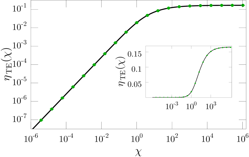
Figure 2: Numerical evaluation of the Casimir–Polder path integral (50) for an atom near a dielectric half-space, relative to the perfect-conductor Casimir–Polder potential $-3\hbar c\alpha_{0}/32\pi^{2}\epsilon_{0}d^{4}$, as a function of the dielectric susceptibility $\chi$, for $N=10^{5}$ points per path, averaged over $10^{8}$ paths. The solid line gives the analytic result (54) for comparison. Error bars delimit one standard deviation. Inset: same data plotted with a linear vertical axis.

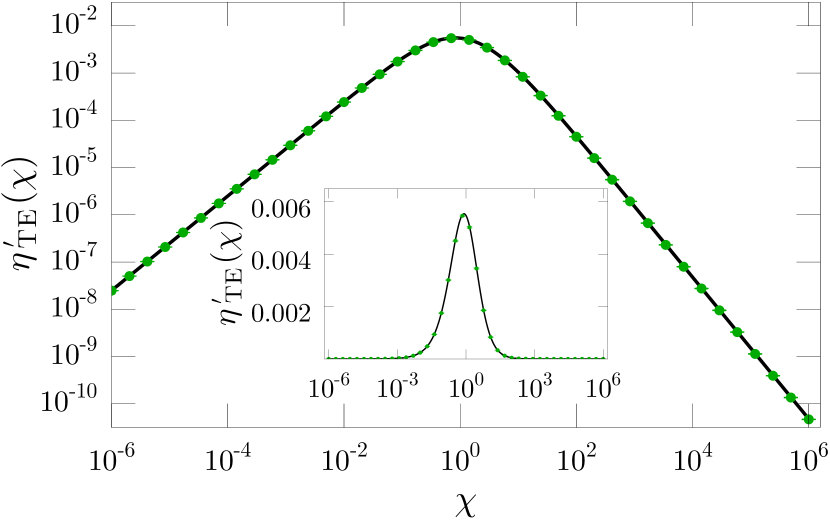
Figure 3: Numerical evaluation of the Casimir–Polder path integral (55) for an atom embedded on the dielectric side of a dielectric half-space, relative to $3\hbar c\alpha_{0}/32\pi^{2}\epsilon_{0}d^{4}$, as a function of the dielectric susceptibility $\chi$, for $N=10^{5}$, averaged over $10^{6}$ paths. The solid line gives the analytic result (58) for comparison. Error bars delimit one standard deviation. Inset: same data plotted with a linear vertical axis.

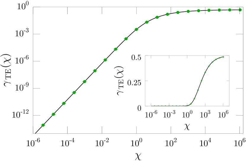
Figure 4: Numerical evaluation of the Casimir-energy path integral (27) for two parallel dielectric half-spaces, normalized to the perfect-conductor energy, as a function of the dielectric susceptibility $\chi$, for $N=10^{5}$, averaged over $10^{8}$ paths. The solid line gives the analytic result (63) for comparison. Error bars delimit one standard deviation. Inset: same data plotted with a linear vertical axis.

The numerical convergence of the Casimir–Polder and Casimir energies is shown in Figs. 5 and 6, respectively, where the numerical estimates $\bar{\eta}_{\mathrm{\scriptscriptstyle TE}}$ and $\bar{\gamma}_{\mathrm{\scriptscriptstyle TE}}$ approach the exact values $\eta_{\mathrm{\scriptscriptstyle TE}}$ and $\gamma_{\mathrm{\scriptscriptstyle TE}}$ as the number of points $N$ per path increases. The plots include data over a range of susceptibilities where the error is largest: $\chi=1$, $10^{2}$, $10^{4}$, and $10^{6}$, as well as the strong–coupling limit $\chi\longrightarrow\infty$. At fixed $N$ the error increases with $\chi$, which is expected because the path average $\langle\epsilon_{\mathrm{r}}\rangle$ can fluctuate over a wider range of values as $\chi$ increases.

The analysis of the scaling of the error with $N$ for such stochastic integrals is nontrivial. Generally, we need to deal with two considerations: the discretization error of the integral in the path average (70), and the truncation error in the derivation of the path integral in Eq. (20). Naively, one could expect that both these errors converge to zero as $N^{-1}$: in Eq. (70) this arises from using the simplest trapezoidal rule, whereas in Eq. (21), there is an additional truncation error that is $O(\smash{N^{-2}})$ for each of the $N$ terms. The numerical data, however, show a more complicated, $\chi$-dependent scaling behavior that we now discuss.

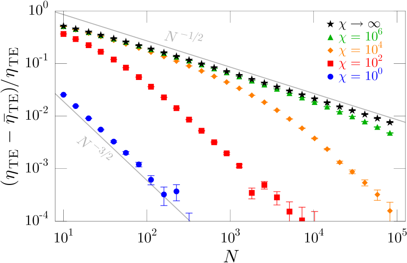
Figure 5: Numerical convergence of the Casimir–Polder path integral (36) for an atom near a dielectric half-space. The relative error is shown as a function of the number $N$ of points per path for various values of $\chi$ as indicated, including the strong-coupling limit $\chi\longrightarrow\infty$. All data points are averaged over $10^{9}$ paths. Grey lines indicated $N^{-3/2}$ and $N^{-1/2}$ scaling behaviors.

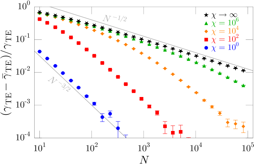
Figure 6: Numerical convergence of the Casimir-energy path integral (27) for two parallel dielectric half-spaces. The relative error is shown as a function of the number $N$ of points per path for various values of $\chi$ as indicated, including the strong-coupling limit $\chi\longrightarrow\infty$. All data points are averaged over $10^{9}$ paths. Grey lines indicated $N^{-3/2}$ and $N^{-1/2}$ scaling behaviors.

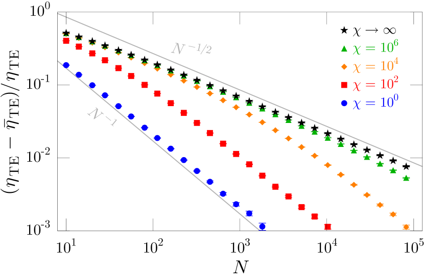
Figure 7: Numerical convergence of the Casimir–Polder path integral (36) for an atom near a dielectric half-space, as in Fig. 5, but using the interpolation estimator (80) instead of the trapezoidal estimator (70). All data points are averaged over $10^{9}$ paths.

The situation is simplest in the limit $\chi\longrightarrow\infty$, which we discuss first. In this limit, the error scales as $N^{-1/2}$. To understand this, note that the integrand of the path integral “saturates” whenever a path crosses the interface. The error made in the path integral stems from overestimating the first-crossing time $\mathcal{T}_{0}$, where the time-scaled path just touches the surface. To quantify this error, we can compare the discrete path that falls just short of touching the interface with the set of continuous-time paths that pass through the same $N$ points $x_{k}$. Some of these continuous paths have more “reach” than the discrete path, and so they have a non-zero probability to touch the surface between the discrete points. The scaling of the error follows from considering a (discrete) path with source point $x_{0}=0$ at distance $d>0$ from the planar interface. The farthest extent of the path towards the interface occurs at some point $x_{n}$, with $x_{n}\propto\smash{\sqrt{\mathcal{T}}}$. The farthest extent becomes $x_{n}=d$ when $\mathcal{T}=\mathcal{T}_{0}$. Then

$$\ell=d\left(1-\sqrt{\frac{\mathcal{T}}{\mathcal{T}_{0}}}\right)$$ (74)

represents the distance between the farthest extent of the path and the interface. For $\mathcal{T}<\mathcal{T}_{0}$, there is no contribution of the discrete path to the path integral. However, even for $\mathcal{T}<\mathcal{T}_{0}$, the continuous paths can still touch the interface. A good approximation of the touching probability is to only consider the intervals between $x_{n}$ and $x_{n\pm 1}$. The scaling behavior of the probability of both these intervals is the same, and for simplicity, we only consider the interval $x_{n}$ to $x_{n+1}$. Since $x_{n}$ is the farthest extent of the path, the probability for the continuous path to touch the interface is maximum when $x_{n+1}=x_{n}$, in which case the probability is given by the crossing probability of a Brownian bridge for a boundary at distance $\ell$ over time $\smash{\Delta\mathcal{T}=\mathcal{T}/N}$. From Eq. (37), this is $\smash{e^{-2\ell^{2}/\Delta\mathcal{T}}}$. Thus, the error in the path integral is, up to an overall factor,

$$e(N)=\int_{0}^{\mathcal{T}_{0}}\!\!\!\frac{d\mathcal{T}}{\mathcal{T}^{1+D/2}}\,\exp\left[-\frac{2Nd^{2}\big{(}1-\sqrt{\mathcal{T}/\mathcal{T}_{0}}\big{)}^{\!2}}{\mathcal{T}}\right].$$ (75)

Defining $\delta\mathcal{T}:=\mathcal{T}_{0}-\mathcal{T}$, the dominant contribution to the integral comes from small $\delta\mathcal{T}$, since large values are exponentially suppressed. Keeping only the leading-order contribution in $\delta\mathcal{T}$, changing integration variables to $\delta\mathcal{T}$, and extending the upper integration limit, the error becomes

$$e(N)\approx \int_{0}^{\infty}\!\!\!\!\frac{d\delta\mathcal{T}}{\mathcal{T}^{1+D/2}_{0}}\,\exp\left[-\frac{2Nd^{2}\delta\mathcal{T}^{2}}{4\mathcal{T}_{0}^{\,3}}\right]$$

$$= \,\sqrt{\frac{\pi}{2d^{2}\mathcal{T}_{0}^{D-1}N}},$$ (76)

which explains the observed $N^{-1/2}$ scaling of the error in the strong-coupling limit.

To understand the scaling in the limit of small $\chi$, we will begin by considering a similar argument. The discrete path underestimates the value of the integrand for $\mathcal{T}$ slightly less than $\mathcal{T}_{0}$, because while the finite-$N$ path does not cross the interface, it may do so in the continuous limit. The estimate for the error in this case is similar to the situation for the large-$\chi$ limit, but involves the sojourn time $T_{\mathrm{s}}$. Again letting $x_{n}$ denote the point in the path with the farthest extent, the contribution of the continuous path between neighboring discrete points $x_{n}=x_{n+1}$ (which we take to be equal for the moment to give a simple estimate) is due to the mean sojourn time of this path segment. In terms of the sojourn time, the error estimate is, up to an overall factor,

$$e(N)=\int_{0}^{\mathcal{T}_{0}}\!\!\!\frac{d\mathcal{T}}{\mathcal{T}^{1+D/2}}\,\mathcal{T}^{-1}{\Big{\langle}\kern-3.50006pt\Big{\langle}}T_{\mathrm{s}}{\Big{\rangle}\kern-3.50006pt\Big{\rangle}},$$ (77)

where the ensemble average here encompasses all continuous paths connecting $x_{n}$ to $x_{n+1}$. The mean sojourn time can be computed from the density (40); the relevant path here is a Brownian bridge spanning time $\Delta\mathcal{T}$, with a boundary at distance $\ell\geq 0$. The result is

$${\Big{\langle}\kern-3.50006pt\Big{\langle}}T_{\mathrm{s}}{\Big{\rangle}\kern-3.50006pt\Big{\rangle}}=\frac{\Delta\mathcal{T}}{2}\,e^{-2\ell^{2}/\Delta\mathcal{T}}-\sqrt{\frac{\pi\ell^{2}\Delta\mathcal{T}}{2}}\,\,\mathrm{erfc}\,\sqrt{\frac{2\ell^{2}}{\Delta\mathcal{T}}}.$$ (78)

Again expanding to lowest order in $\delta\mathcal{T}:=\mathcal{T}_{0}-\mathcal{T}$ changing integration variables, and extending the upper integration limit to infinity, the error becomes

$$\begin{array}[]{l}\displaystyle e(N)\approx\int_{0}^{\infty}\!\!\!\frac{d\delta\mathcal{T}}{\mathcal{T}_{0}^{2+D/2}}\Bigg{[}\frac{\mathcal{T}_{0}}{2N}\,e^{-Nd^{2}\delta\mathcal{T}^{2}/2\mathcal{T}_{0}^{\,3}}\\ \displaystyle\hskip 73.97716pt{}-\sqrt{\frac{\pi d^{2}\delta\mathcal{T}^{2}}{8N\mathcal{T}_{0}}}\,\,\mathrm{erfc}\,\sqrt{\frac{Nd^{2}\delta\mathcal{T}^{2}}{2\mathcal{T}_{0}^{\,3}}}\Bigg{]}\\ \displaystyle\hskip 24.18483pt=\sqrt{\frac{\pi}{32d^{2}\mathcal{T}_{0}^{D-1}N^{3}}}.\end{array}$$ (79)

The resulting error estimate scales as $N^{-3/2}$, as observed in the numerical data. However, this argument is incomplete, as it ignores the important case when a path segment straddles the interface, and it also ignores the contribution of the other path segments.

The main use of this argument is to provide a heuristic explanation of the crossover between different scaling behaviors for finite $\chi$ and with increasing $N$. In the small-$\chi$ limit, the error associated with the first path segment touching the boundary has an $O(N^{-1/2})$ component due to the extent of the segment, as in the large-$\chi$ limit, but each segment can only make an $O(N^{-1})$ contribution relative to the total path. This extra $O(N^{-1})$ contribution does not matter if $\chi$ is arbitrarily large, since even a single path segment crossing the interface causes the integrand to saturate, leading to the $N^{-1/2}$ scaling in this regime. For any finite $N$, there should then be a crossover between these scaling behaviors, because it is only when $\chi/N\gg 1$ that the sojourn-time contribution of the subpath saturates the integrand, whereas the small-chi limit corresponds to $\chi/N\ll 1$. Thus we expect a crossover between $N^{-1/2}$ to $N^{-3/2}$ error scaling around $N\sim\chi$, as observed in the numerical data above. In particular, based on the numeric results, this means that for any finite $\chi$, the error scales asymptotically with the faster $N^{-3/2}$ power law after passing through the crossover regime.

In fact, the $N^{-3/2}$ error scaling is somewhat surprising: as noted above, the discretization error of the path-average estimator (70) suggests that the error should scale no better than $N^{-1}$. To better understand this scaling behavior, it is necessary to consider the contribution of the entire path. In doing so, it is useful to compare different approximations for the path average. For example, an alternate estimator arises via

$$\begin{array}[]{rcl}\!\left\langle{\epsilon_{\mathrm{r}}}\right\rangle&{}={}&\displaystyle\frac{1}{\mathcal{T}}\sum_{j=0}^{N-1}\int_{\mathcal{T}_{j}}^{\mathcal{T}_{j+1}}\!\!\!\!d\tau\,\epsilon_{\mathrm{r}}[x(\tau)]\\ &{}\approx{}&\displaystyle\frac{1}{\mathcal{T}}\sum_{j=0}^{N-1}\int_{x_{j}}^{x_{j+1}}\!\!\!\!dx\,\epsilon_{\mathrm{r}}(x)\,\frac{\Delta\mathcal{T}}{\Delta x_{j}}\\ &{}={}&\displaystyle\frac{1}{N}\sum_{j=0}^{N-1}\frac{1}{\Delta x_{j}}\int_{x_{j}}^{x_{j+1}}\!\!\!\!dx\,\epsilon_{\mathrm{r}}(x),\end{array}$$ (80)

where $\Delta x_{j}=x_{j+1}-x_{j}$ and $\mathcal{T}_{j}:=j\Delta\mathcal{T}$. The final summand here is the average integrated value of $\epsilon_{\mathrm{r}}(x)$ between $x_{j}$ and $x_{j+1}$ (in multiple spatial dimensions, this is the average value computed along the straight line connecting $\mathbf{x}_{j}$ and $\mathbf{x}_{j+1}$). The integrals here can be computed straightfowardly for a dielectric interface in terms of the fraction of the straight-line interval spent past the interface. The reference method (70) can be written

$$\!\left\langle{\epsilon_{\mathrm{r}}}\right\rangle=\frac{1}{N}\sum_{j=0}^{N-1}\frac{\epsilon_{\mathrm{r}}(x_{j})+\epsilon_{\mathrm{r}}(x_{j+1})}{2}$$ (81)

because $x_{N}=x_{0}$, and this method coincides with the ordinary trapezoidal rule in numerical quadrature. For a smooth, deterministic integrand, both methods have an error that scales as $N^{-2}$. However, in computing a sojourn-time integral, the error estimate is complicated by the involvement of a stochastic path as well as a discontinuous integrand. As it turns out, the interpolation method (80) achieves the worst-case $N^{-1}$ asymptotic scaling that we noted above. This is shown in Fig. 7, which is the same calculation as in Fig. 5, except in using the interpolation rule (80) instead of the trapezoidal rule (81).

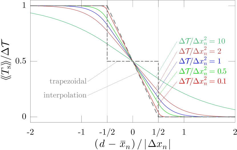
Figure 8: Average sojourn time $\langle\!\langle{T_{\mathrm{s}}}\rangle\!\rangle$ for one path segment from $x_{n}$ to $x_{n+1}$ [Eq. (125)] plotted as a function of the interface location $d$. The horizontal axis is shifted such that the interval midpoint $\bar{x}_{n}:=(x_{n}+x_{n+1})/2$ is centered in the plot, and the axis is scaled such that the interval boundaries $x_{n}$ and $x_{n+1}$ are located at $\pm 1/2$, as marked by thin vertical lines. The trapezoidal and interpolation estimators for the sojourn time, given respectively by Eqs. (81) and (80), are superimposed for comparison. Note that the mean sojourn time decreases monotonically with $d$ because the path has less opportunity to sojourn in the region to the right of $d$.

On the other hand, the trapezoidal rule performs substantially better. The difference between the interpolation rule and the trapezoidal rule lies entirely in the case where the points $x_{n}$ and $x_{n+1}$ straddle the interface, a case ignored by the error estimate (79). The mean sojourn time for a bridge between $x_{n}$ and $x_{n+1}$ may be calculated from the probability density in Eq. (125). The results are visualized in Fig. 8. The figure also shows the functions approximating $\langle\!\langle{T_{\mathrm{s}}}\rangle\!\rangle$, corresponding to the interpolation rule and the trapezoidal rule. Note that the interpolation rule appears to be a good approximation for $\langle\!\langle{T_{\mathrm{s}}}\rangle\!\rangle$ for small values of $\Delta\mathcal{T}/\Delta x_{n}^{\,2}$, which correspond to very long (albeit rare) steps, where the Brownian path is close to a straight-line (classical) path. The trapezoidal-rule curve does not obviously constitute any kind of good approximation to any of the sojourn-time curves. The main feature to note from this plot is that, outside of the region between $x_{n}$ and $x_{n+1}$, the curves all have important common features: they share the same reflection symmetry, and they decay exponentially to zero or one in essentially the same way (once the scaling in the plot is accounted for) as the case when $x_{n}=x_{n+1}$. Thus, a heuristic estimate for the error scaling follows by adapting the error expression (79), which assumes $x_{n}=x_{n+1}$, as follows. The estimate only accounted for the error on the leading side of the path segment. If we also account for the error on the trailing side, which amounts to extending the lower integration limit to $-\infty$, the resulting expression vanishes. Then the leading-order result comes from keeping the first-order term in $\delta\mathcal{T}$ from the expansion of the $\mathcal{T}^{-(1+D/2)}$ factor. The resulting integral gives an error that scales as $N^{-2}$. However, there are $N$ total path segments, so the overall error scales as $N^{-1}$, which matches the simple error estimate from the $N$-point discretization of the path. This $N^{-1}$ scaling also applies, for example, to a midpoint rule $\epsilon_{\mathrm{r}}(\bar{x}_{j})$ in place of the two-point average in the sum of Eq. (81), or to any other estimator that depends on $\epsilon_{\mathrm{r}}(\mathbf{r})$ along the straight line between $x_{n}$ and $x_{n+1}$, except for the trapezoidal rule.

Then what is special about the trapezoidal rule? It turns out to have the following remarkable property: when averaged over all possible steps $\Delta x_{n}$, the trapezoidal rule can exactly reproduce the mean sojourn time. Mathematically, consider the mean sojourn time, Eq. (125), with $a=-\Delta x_{n}/2$, $c=\Delta x_{n}/2$, and $t=\Delta\mathcal{T}$, for Brownian bridges $B_{(-\Delta x_{n}/2)\rightarrow(\Delta x_{n}/2)}(\Delta\mathcal{T})$ connecting $-\Delta x_{n}/2$ to $\Delta x_{n}/2$ in time $\Delta\mathcal{T}$:

$$\begin{array}[]{rcl}&&\displaystyle\overline{{\big{\langle}\kern-2.29996pt\big{\langle}}{T_{\mathrm{s}}}{\big{\rangle}\kern-2.29996pt\big{\rangle}}}:=\int_{-\infty}^{\infty}\!\!d\Delta x_{n}\,\frac{e^{-\Delta x_{n}^{\,2}/2\Delta\mathcal{T}}}{\sqrt{2\pi\Delta\mathcal{T}}}\\ &&\displaystyle{}\hskip 28.45274pt\times{\Big{\langle}\kern-3.50006pt\Big{\langle}}{T_{\mathrm{s}}[B_{(-\Delta x_{n}/2)\rightarrow(\Delta x_{n}/2)}(\Delta\mathcal{T});d]}{\Big{\rangle}\kern-3.50006pt\Big{\rangle}}\end{array}$$ (82)

The overbar here denotes the average over all possible steps $\Delta x_{n}$, weighted by the Gaussian probability density for the step, and the step interval is centered ($\bar{x}_{n}=0$) to simplify the notation. Using the estimator $\smash{\langle\!\langle{\tilde{T}_{\mathrm{s}}}\rangle\!\rangle}$ corresponding to the trapezoidal rule, the analogous average is

$$\begin{array}[]{rcl}&&\displaystyle\overline{{\big{\langle}\kern-2.29996pt\big{\langle}}{\tilde{T}_{\mathrm{s}}}{\big{\rangle}\kern-2.29996pt\big{\rangle}}}=\int_{-\infty}^{\infty}\!\!d\Delta x_{n}\frac{e^{-\Delta x_{n}^{\,2}/2\Delta\mathcal{T}}}{\sqrt{2\pi\Delta\mathcal{T}}}\\ &&\displaystyle{}\hskip 28.45274pt\times\frac{\Delta\mathcal{T}}{2}\left[\Theta\bigg{(}\frac{\Delta x_{n}}{2}-d\bigg{)}+\Theta\bigg{(}-\!\frac{\Delta x_{n}}{2}-d\bigg{)}\right]\\ &&\displaystyle{}\hskip 55.48286pt=\frac{\Delta\mathcal{T}}{2}\,\mathrm{erfc}\!\left[\frac{\sqrt{2}\,d}{\sqrt{\Delta\mathcal{T}}}\right],\end{array}$$ (83)

which ends up being exactly the same as the result of evaluating the integral in Eq. (82). When one carries out a more careful calculation of the error, analogous to Eq. (79) but including the difference between the mean sojourn time (125) and the trapezoidal or interpolating estimator (i.e., with $x_{n}\neq x_{n+1}$ in general), as outlined in the previous paragraph, the results are as follows. In the case of the trapezoidal estimator, one finds that for any given step size $\Delta x_{n}$ there is a local error of $O(N^{-2})$, which vanishes when averaged over step sizes as in Eq. (82). When the path segment straddles the interface, the interpolating estimator introduces an excess $O(N^{-2})$ error. With $N$ total path segments, this explains the $O(N^{-1})$ error scaling for the interpolating estimator, and the higher-order error scaling for the trapezoidal estimator.

V.4 Accelerated-convergence techniques

The statistical error due to averaging a finite number of paths is unavoidable. However, for a finite number of points $N$ per path, it is possible to use more sophisticated methods to enhance the accuracy relative to the performance discussed in the previous section. Here we will discuss two such methods in the context of the Casimir–Polder path integral, but the same techniques also apply in the general Casimir case. One method comes from rewriting the TE Casmir–Polder path integral (36) in the (unrenormalized) form

$$V_{\mathrm{\scriptscriptstyle CP}}^{\mathrm{\scriptscriptstyle(TE)}}(\mathbf{r})=\frac{\hbar c\alpha_{0}}{(2\pi)^{D/2}\sqrt{\pi}\epsilon_{0}}\int_{0}^{\infty}\!\!\,\frac{d\mathcal{T}}{\mathcal{T}^{1+D/2}}\,\int_{0}^{\infty}\!\!ds\,s^{2}\,e^{-s^{2}}\,$$

$$\hskip 85.35826pt\times{\Bigg{\langle}\kern-3.50006pt\Bigg{\langle}}\exp\!\Big{[}-\!s^{2}\!\left\langle{\chi}\right\rangle\Big{]}{\Bigg{\rangle}\kern-3.50006pt\Bigg{\rangle}}_{\mathbf{x}(\tau)}\!\!\!\!.$$ (84)

This expression turns out to be the Casimir–Polder analogue of the the Casimir free energy for dispersive media in Eq. (95), if the dependence of the susceptibility on the imaginary frequency is incorporated as $\chi(\mathbf{r})\longrightarrow\chi(\mathbf{r},is)$. If the paths here refer to $N$-point discrete paths, the path average can be written in terms of the components on each path segment as

$$V_{\mathrm{\scriptscriptstyle CP}}^{\mathrm{\scriptscriptstyle(TE)}}(\mathbf{r})=\frac{\hbar c\alpha_{0}}{(2\pi)^{D/2}\sqrt{\pi}\epsilon_{0}}\int_{0}^{\infty}\!\!\,\frac{d\mathcal{T}}{\mathcal{T}^{1+D/2}}\,\int_{0}^{\infty}\!\!ds\,s^{2}\,e^{-s^{2}}\,$$

$$\hskip 34.1433pt\times{\Bigg{\langle}\kern-3.50006pt\Bigg{\langle}}\prod_{j=0}^{N-1}\exp\!\Bigg{[}-\!\frac{s^{2}}{\mathcal{T}}\,\int_{\mathcal{T}_{j}}^{\mathcal{T}_{j+1}}\!\!d\tau\,\chi(\mathbf{x}(\tau))\Bigg{]}{\Bigg{\rangle}\kern-3.50006pt\Bigg{\rangle}}_{\mathbf{x}(\tau)}\!\!\!\!.$$ (85)

For a vacuum–dielectric interface, the integral in the exponential gives the sojourn time in the dielectric of a Brownian bridge connecting $\mathbf{x}_{j}$ to $\mathbf{x}_{j+1}$ in time $\Delta\mathcal{T}$. Instead of estimating the path-segment integrals by using samples $\chi(\mathbf{x}_{j})$ as in the trapezoidal rule (81), it is most accurate to treat the integrals in terms of the Brownian bridge between $\mathbf{x}_{j}$ and $\mathbf{x}_{j+1}$. Averaging over all such bridges results in the exact (in the $N\longrightarrow\infty$ sense) expression

$$V_{\mathrm{\scriptscriptstyle CP}}^{\mathrm{\scriptscriptstyle(TE)}}(\mathbf{r})=\frac{\hbar c\alpha_{0}}{(2\pi)^{D/2}\sqrt{\pi}\epsilon_{0}}\int_{0}^{\infty}\!\!\,\frac{d\mathcal{T}}{\mathcal{T}^{1+D/2}}\,\int_{0}^{\infty}\!\!ds\,s^{2}\,e^{-s^{2}}\,$$

$$\hskip 2.84526pt\times{\Bigg{\langle}\kern-3.50006pt\Bigg{\langle}}\prod_{j=0}^{N-1}{\kern 0.0pt\Bigg{\langle}\kern-6.60004pt\scalebox{0.66}[1.0]{$-$}\kern-2.20001pt\Bigg{\langle}\kern 0.0pt}\exp\!\Bigg{[}-\!\frac{s^{2}}{\mathcal{T}}\,\int_{\mathcal{T}_{j}}^{\mathcal{T}_{j+1}}\!\!d\tau\,\chi(\mathbf{x}(\tau))\Bigg{]}{\kern 0.0pt\Bigg{\rangle}\kern-2.20001pt\scalebox{0.66}[1.0]{$-$}\kern-6.60004pt\Bigg{\rangle}\kern 0.0pt}_{\!\!\Delta x_{j}}{\Bigg{\rangle}\kern-3.50006pt\Bigg{\rangle}}_{\mathbf{x}(\tau)}\!\!\!\!,$$ (86)

where the connected-double-angle brackets $\smash{{\langle\kern-2.79999pt\scalebox{0.35}[1.0]{$-$}\kern-1.79993pt\langle}\;{\rangle\kern-1.79993pt\scalebox{0.35}[1.0]{$-$}\kern-2.79999pt\rangle}_{\Delta x_{j}}}$ denote the ensemble average over all bridges between $\smash{\mathbf{x}_{j}}$ and $\smash{\mathbf{x}_{j+1}}$. The ensemble-averaged exponential factors here then have the form of the generating function of the sojourn time. For a planar vacuum–dielectric interface, expressions for these generating functions appear in Eqs. (B)–(124). The results there are adapted to the present case by identifying $a\longrightarrow x_{j}$, $c\longrightarrow x_{j+1}$, $t\longrightarrow\Delta\mathcal{T}$, and $s\longrightarrow s^{2}\chi/\mathcal{T}$. Thus, for a planar interface, a calculation performed this way has no finite-$N$ discretization error. In fact, the analytic calculation of the TE Casimir–Polder potential in Section IV.2 is essentially a summation of these paths with $N=1$. The expressions for the moment-generating functions involve integrals, but they can be evaluated over the range of necessary values in the two free variables: the scaled interval length $(c-a)/\sqrt{t}$ and the scaled boundary location $(d-a)/\sqrt{t}$. The values needed in evaluating the path integral can then be generated as needed from an interpolation table in these two variables.

The other method applies to the original path integral (36) for the Casimir–Polder potential, where the goal is to accurately evaluate the path average $\,\!\left\langle{\epsilon_{\mathrm{r}}}\right\rangle$. Writing out the path average as

$$\!\left\langle{\epsilon_{\mathrm{r}}}\right\rangle=1+\frac{1}{\mathcal{T}}\sum_{j=0}^{N-1}\int_{\mathcal{T}_{j}}^{\mathcal{T}_{j+1}}\!\!\!\!d\tau\,\chi[x(\tau)],$$ (87)

the integrals here again have the form of the sojourn time in the dielectric medium, in the case of a uniform dielectric with a sharp boundary. The approach of Eq. (86), where the sojourn-time integrals for the path segments are replaced by the ensemble averages over Brownian bridges connecting $\mathbf{x}_{j}$ to $\mathbf{x}_{j+1}$, is possible here by employing Eq. (125), but not optimal. However, since the probability density for the sojourn time is known in Eqs. (116)–(116), these integrals can be interpreted as random variables, chosen according to the sojourn-time probability density. The expression for the sojourn density is relatively complicated, but the only free parameters are the scaled interval length $(c-a)/\sqrt{t}$, the scaled boundary location $(d-a)/\sqrt{t}$, and the sojourn time $x/t$. It is thus feasible to compute all necessary values of the inverse cumulative probability function, generating deviates via an interpolation table in three variables. The same idea has been applied in financial mathematics, for example, in the pricing of occupation-time derivatives Makarov and Wouterloot (2012). Again, for a planar interface, this method corresponds to directly taking the limit $N\longrightarrow\infty$, with any finite-$N$ path. The analytic calculation of the TE path integral described following Eq. (40) via the sojourn-time distribution is equivalent to a summation over paths in this method for $N=1$.

Of course, the planar-interface solution of the path integral is already known. The real value of these methods lies in evaluating the path integrals with interfaces of arbitrary geometry. These methods will still dramatically reduce the discretization error in the general case, provided $N$ is large enough that the interface is well-approximated by a plane on the length scale of a path segment. In this case, the planar-geometry expressions for the sojourn-time distributions can be employed. For example, these methods are already approximate in the case of two parallel, planar interfaces, because each path segment is assumed to only interact with one plane; however, this is an excellent approximation provided that $\sqrt{\Delta\mathcal{T}}$ is small compared to the gap between the interfaces. These methods would be especially beneficial in the perfect-conductor (Dirichlet-boundary) limit, where the asymptotic convergence with $N$ is particularly slow.

VI Non-zero Temperature and Dispersion

In considering scenarios more relevant to experiments, it is important to incorporate material dispersion and nonzero temperatures. Here we will discuss the generalization of the worldline formalism to dispersive dielectric materials at nonzero temperature. Such effects were already incorporated in the early work of Dzyaloshinskii et. al Dzyaloshinskii and Pitaevskii (1959); Dzyaloshinskii, Lifshitz, and Pitaevskii (1961). However, electromagnetic quantization with dispersive materials requires some care and has thus been the subject of much study, because causality considerations imply that dispersive materials are also absorptive. Dispersive quantization is typically handled by coupling the electromagnetic field to an idealized, linear medium, and then coupling the medium to a bath of oscillators that models dissipation Huttner and Barnett (1992); Dung, Knöll, and Welsch (1998); Bechler (1999). A similar approach, outlined in Appendix A of Ref. Rahi et al. (2009), emphasizes that the dielectric constant is related to the linear response of the underlying medium. For a linear medium, one can carefully calculate the total energy for total medium–bath system, including energy lost to dissipation. This procedure leads to expressions for the Casimir energy that correspond to results computed in the absence of dispersion, but with the substitution $\epsilon\rightarrow\epsilon(i\omega)$ Barash and Ginzburg (1975); Rosa, Dalvit, and Milonni (2010, 2011).

The common theme of this prior work is that the dependence of Casimir energies on dielectric media enters solely via the imaginary-frequency permittivity $\epsilon_{\mathrm{r}}(\mathbf{r},is_{n})$ evaluated at the Matsubara frequencies $s_{n}:=2\pi n/\hbar\beta$. To sketch how this comes about in the path integral, first note that the Wick-rotated scalar field $\phi(\mathbf{x},\tau)$ from the partition function (11) can be expanded in a Fourier series as

$$\phi(\mathbf{r},\tau)=\sum_{n=-\infty}^{\infty}\phi_{n}(\mathbf{r})\,e^{-is_{n}\tau/c},$$ (88)

where

$$\phi_{n}(\mathbf{r})=\int_{0}^{\beta\hbar c}\!\!d\tau\,e^{is_{n}\tau/c}\,\phi(\mathbf{r},\tau).$$ (89)

In this expression the Wick rotation has replaced the real frequency by $\omega_{n}\longrightarrow is_{n}$. Putting this expression for $\phi(\mathbf{r},\tau)$ into the partition function (11), we can introduce material dispersion by giving $\epsilon_{\mathrm{r}}$ the proper frequency dependence for each Matsubara mode. The result with $\mu_{\mathrm{r}}=1$ is

$$Z_{\mathrm{\scriptscriptstyle TE}}= \prod_{n=-\infty}^{\infty}\int\!D\phi_{n}\exp\left[-\frac{\epsilon_{0}c}{2\hbar}\int d\mathbf{r}\right.$$

$$\left.\times\left(\epsilon_{\mathrm{r}}(\mathbf{r},is_{n})\frac{s_{n}^{2}}{c^{2}}|\phi_{n}(\mathbf{r})|^{2}+|\nabla\phi_{n}(\mathbf{r})|^{2}\right)\right],$$ (90)

where the temperature dependence is implicit in the $s_{n}$. With nonzero temperature, the appropriate thermodynamic quantity for computing forces is the free energy, given by $\mathcal{F}=-\beta^{-1}\log Z$, which is equivalent to the mean energy in the limit $\beta\longrightarrow\infty$. After integration over the fields in the partition functions, the free energy becomes

$$\mathcal{F}=-\beta^{-1}{\sum_{n}}^{\prime}\log\det\left[\epsilon_{\mathrm{r}}(\mathbf{r},is_{n})\frac{s_{n}^{2}}{c^{2}}-\nabla^{2}\right],$$ (91)

where the primed summation is defined by ${\sum^{\prime}_{n}}f_{n}:=\frac{1}{2}f_{0}+\sum_{n=1}^{\infty}f_{n}$. The development of the worldline path integral proceeds in the same manner as in Section (III), with the unrenormalized result

$$\mathcal{F}= -\!\frac{1}{(2\pi)^{(D-1)/2}\beta}\,{\sum_{n}}^{\prime}\int_{0}^{\infty}\!\!\frac{d\mathcal{T}}{\mathcal{T}^{(D+1)/2}}\int d\mathbf{x}_{0}$$

$$\hskip 42.67912pt{}\times{\Big{\langle}\kern-3.50006pt\Big{\langle}}e^{-s_{n}^{2}\langle\epsilon_{\mathrm{r}}(\mathbf{x},is_{n})\rangle\mathcal{T}/(2c^{2})}{\Big{\rangle}\kern-3.50006pt\Big{\rangle}}_{\mathbf{x}(t)}.$$ (92)

The unrenormalized thermal Casimir–Polder energy follows according to the logic of Section (III.2), with the result

$$V_{\mathrm{\scriptscriptstyle CP}}(\mathbf{r}_{\mathrm{\scriptscriptstyle A}},\beta)= \,\frac{1}{2(2\pi)^{(D-1)/2}\epsilon_{0}c^{2}\beta}\,{\sum_{n}}^{\prime}s_{n}^{2}\,\alpha(is_{n})$$

$$\times\!\int_{0}^{\infty}\!\!\frac{d\mathcal{T}}{\mathcal{T}^{(D-1)/2}}{\bigg{\langle}\kern-3.50006pt\bigg{\langle}}e^{-s_{n}^{\,2}\langle\epsilon_{\mathrm{r}}(\mathbf{x},is_{n})\rangle\mathcal{T}/(2c^{2})}{\bigg{\rangle}\kern-3.50006pt\bigg{\rangle}}_{\mathbf{x}(t)}\!.$$ (93)

Note that in both cases the path average $\langle\epsilon_{\mathrm{r}}\rangle$ is exponentiated, like a path-integral potential, in contrast to the $\langle\epsilon_{\mathrm{r}}\rangle^{-\alpha}$ forms of the dispersion-free path integrals. Also, since $\epsilon_{\mathrm{r}}(\mathbf{r},is_{n})$ is real and positive for a causal medium, the exponential factors here are well-behaved.

In the limit of high temperature, the only contribution to the Casimir–Polder potential comes from the lowest Matsubara mode at frequency $s_{0}=0$. However, due to the presence of the factor $s_{n}^{\,2}$ in Eq. (93), this potential vanishes. This is consistent with known results for a planar interface Babb, Klimchitskaya, and Mostepanenko (2004), where in the limit of high temperature the leading-order contribution to the potential comes only from the TM polarization.

In both the Casimir and Casimir–Polder path integrals, the zero-temperature limit emerges as the Matsubara sum becomes well-approximated by an integral over frequency. Making the replacement

$$\frac{2\pi}{\hbar\beta}\,\,{\sum_{n}}^{\prime}\longrightarrow\int_{0}^{\infty}\!\!ds,$$ (94)

so that, for example, the Casimir free energy becomes

$$\mathcal{F}= -\!\frac{\hbar}{(2\pi)^{(D+1)/2}}\int_{0}^{\infty}\!\!ds\int_{0}^{\infty}\!\!\frac{d\mathcal{T}}{\mathcal{T}^{(D+1)/2}}\int\!d\mathbf{x}_{0}$$

$$\hskip 71.13188pt{}\times{\bigg{\langle}\kern-3.50006pt\bigg{\langle}}e^{-s^{2}\mathcal{T}\langle\epsilon_{\mathrm{r}}(\mathbf{x},is)\rangle/2c^{2}}{\bigg{\rangle}\kern-3.50006pt\bigg{\rangle}}_{\mathbf{x}_{0}}.$$ (95)

Note that the $s$ integration in Eq. (49), which exponentiated the $\langle\epsilon_{\mathrm{r}}\rangle^{-\alpha}$ dependence on the dielectric, plays essentially the same role as the integral over the imaginary frequency $s$ here, but now this integration has a physical interpretation. In the far-field limit, where the dominant transition wavelengths $\omega/c$ are small relative to the separation of objects, the dielectric permittivity is given approximately by its zero-frequency value. Then, after carrying out the integral over $s$, the path integral reduces to the dispersion-free expression in Eq. (24) with $\mu_{r}\longrightarrow 1$.

VII Summary

We have extended the worldline method for scalar-field Casimir energies to better model electromagnetism, by incorporating a coupling of the field to the dielectric permittivity $\epsilon_{\mathrm{r}}(\mathbf{r})$ and magnetic permeability $\mu_{\mathrm{r}}(\mathbf{r})$. We have also discussed the extension of the path integrals to dispersive media at nonzero temperature.

The numerical evaluation of the Casimir and Casimir–Polder energies in planar geometries, where exact results are known, demonstrates the good convergence properties of the path integrals. This agreement should also extend to other geometries where the polarizations decouple. The numerical methods apply in arbitrary geometries, giving Casimir energies for a scalar field coupled to a magnetodielectric material. They also serve as a scalar approximation for the full electromagnetic Casimir energy in arbitrary geometries.

We have also demonstrated analytically that the worldline path integrals developed here converge to the correct values for both Casimir and Casimir–Polder energies in planar geometries. The analytical techniques developed here are also useful for handling the more technically challenging case of the TM polarization, in both analytic and numerical calculations, which we will discuss in future work Mackrory, Bhattacharya, and Steck (tion).

VIII Acknowledgments

The authors thank Richard Wagner and Wes Erickson for comments on the manuscript. This research was supported by NSF grants PHY-1068583 and PHY-1505118.

Appendix A Solutions to Feynman-Kac formulae

In the analytic summations of worldlines in Section IV, the solutions to the differential equation (44) are required to give explicit expressions to the ensemble average (43) over paths. Here we will give an overview of the derivation of explicit expressions that correspond to either one or two dielectric half-spaces. Recall that only the solution $f(x)$ at $x=0$ is required, as this is the case that generates an average over closed paths, as required by the trace in Eq. (17).

A.1 One-step potential

The potential corresponding to a single dielectric half-space of susceptibility $\chi$ is

$$V(x)=\chi\Theta(x-d),$$ (96)

where $d$ is the distance to the planar interface. A path source point on the vacuum side of the interface corresponds to $d>0$, while a source point on the dielectric side corresponds to $d<0$. Written out explicitly, the differential equation (44) to solve is

$$f^{\prime\prime}(x)=2\big{[}\lambda+\chi\Theta(x-d)\big{]}\,f(x)-2\delta(x),$$ (97)

and the solution gives the path average

$$f(0)=\int_{0}^{\infty}\!\!dt^{\prime}\,{\bigg{\langle}\kern-3.50006pt\bigg{\langle}}\delta[W(t^{\prime})]\,e^{-\lambda t^{\prime}-\chi\int_{0}^{t^{\prime}}\!dt^{\prime\prime}\,\Theta[x(t^{\prime\prime})-d]}{\bigg{\rangle}\kern-3.50006pt\bigg{\rangle}},$$ (98)

where again the double angle brackets $\langle\!\langle\cdots\rangle\!\rangle$ denote an average over Wiener paths, which are forced to close here by the delta function.

The solutions to Eq. (97) are linear combinations of the functions $\smash{\exp[{\pm\sqrt{2\lambda}\,x}]}$ in regions where $x<d$, and of $\smash{\exp[{\pm\sqrt{2(\lambda+\chi)}\,x}]}$ in regions where $x>d$. Then the solution is determined by enforcing continuity of $f(x)$ and $f^{\prime}(x)$ across the interface at $x=d$, enforcing a jump in $f^{\prime}(x)$ at $x=0$ due to the delta function,

$$f^{\prime}(0_{+})-f^{\prime}(0_{-})=-2,$$ (99)

while enforcing continuity of $f(x)$ itself, and finally requiring $f(x)\longrightarrow 0$ as $x\longrightarrow\pm\infty$. With these conditions, the solution is

$$f(0)=\left\{\begin{array}[]{ll}\dfrac{1}{\sqrt{2\lambda}}\left(1+r\,e^{-2\sqrt{2\lambda}\,d}\right)&(d>0)\\ \dfrac{1}{\sqrt{2(\lambda+\chi)}}\left(1-r\,e^{2\sqrt{2(\lambda+\chi)}\,d}\right)&(d<0),\\ \end{array}\right.$$ (100)

where

$$r=\frac{\sqrt{\lambda}-\sqrt{\lambda+\chi}}{\sqrt{\lambda}+\sqrt{\lambda+\chi}}$$ (101)

has the form of the Fresnel reflection coefficient for TE polarization at a vacuum–dielectric interface (provided that in terms of the angle of incidence $\theta$ from the vacuum side, one identifies $\lambda=\cos^{2}\theta$).

Combining Eqs. (98) and (100) and applying the logic of Eqs. (22) and (23) to remove the delta function, the result is

$$\int_{0}^{\infty}\!\!\frac{d\mathcal{T}}{\sqrt{\mathcal{T}}}\,e^{-\lambda\mathcal{T}}{\bigg{\langle}\kern-3.50006pt\bigg{\langle}}e^{-\chi\int_{0}^{\mathcal{T}}dt\,\Theta[x(t)-d]}{\bigg{\rangle}\kern-3.50006pt\bigg{\rangle}}_{x(t)}$$

$$=\sqrt{\frac{\pi}{\lambda+\chi\Theta(-d)}}\left[1+\mathrm{sgn}(d)\,r\,e^{-2\sqrt{2[\lambda+\chi\Theta(-d)]}\,|d|}\right],$$ (102)

where the paths $x(t)$ are now restricted to Brownian bridges, satisfying $x(0)=x(\mathcal{T})=0$. This solution is then useful in computing the Casimir–Polder potential for an atom near a planar dielectric interface, by providing an expression for the $\mathcal{T}$ integral in Eq. (49). For example, for $d>0$ the replacements $\chi\longrightarrow s\chi$ and $\lambda\longrightarrow\lambda+s$ in Eq. (102) give Eq. (51).

This result is also useful in computing the Casimir energy of two dielectric half-spaces, where the integral of Eq. (102) over all path source points $x_{0}$ represents the one-body energy of each half-space. Since the source point is $x_{0}=0$ in Eq. (102), it is easiest to interpret $d$ as the distance from the source point to the interface, and thus the replacement $d\longrightarrow d-x_{0}$ explicitly restores the source-point dependence,

$$\int_{0}^{\infty}\!\!\frac{d\mathcal{T}}{\sqrt{\mathcal{T}}}\,e^{-\lambda\mathcal{T}}{\bigg{\langle}\kern-3.50006pt\bigg{\langle}}e^{-\chi\int_{0}^{\mathcal{T}}dt\,\Theta[x(t)-d]}{\bigg{\rangle}\kern-3.50006pt\bigg{\rangle}}_{x(t)}$$

$$=\sqrt{\frac{\pi}{\lambda+\chi\Theta(x_{0}-d)}}$$

$$\hskip 14.22636pt\times{}\left[1+\mathrm{sgn}(d-x_{0})\,r\,e^{-2\sqrt{2[\lambda+\chi\Theta(x_{0}-d)]}\,|d|}\right],$$ (103)

where now $x(0)=x(\mathcal{T})=x_{0}$. The first term on the right-hand side vanishes under renormalization, represented by the subtractions in the last two terms in Eq. (59), which amounts to subtracting away ultraviolent divergences as $\mathcal{T}\longrightarrow 0$. The remaining integral over $x_{0}$ yields the one-body contribution

$$I=\left(\frac{1}{4\lambda}-\frac{1}{4(\lambda+\chi)}\right)r$$ (104)

to the total energy. This result is useful in subtracting the one-body contributions from the two-body interaction energy in Eq. (59), leading to the last two terms in the last factor in Eq. (60).

A.2 Two-step potential

The potential corresponding to two dielectric half-spaces with separation $d$ and susceptibilities $\chi_{1}$ for $x<d_{1}$ and $\chi_{2}$ for $x>d_{2}$ is

$$V(x)=\chi_{1}\Theta(d_{1}-x)+\chi_{2}\Theta(x-d_{2}),$$ (105)

where $d=d_{2}-d_{1}>0$. Following the method in the previous section for the one-step potential, the differential equation (44) to solve is

$$f^{\prime\prime}(x)=2\big{[}\lambda+\chi_{1}\Theta(d_{1}-x)+\chi_{2}\Theta(x-d_{2})\big{]}\,f(x)-2\delta(x).$$ (106)

Applying the same conditions as in the one-step case, the solution $f(0)$ may be written in three distinct regions. For $0<d_{1}<d_{2}$, the solution corresponds to path source points in the $\chi_{1}$ dielectric region $x_{0}<d_{1}$, and is given by

$$f_{\text{I}}(0) =\dfrac{1}{\sqrt{2(\lambda+\chi_{1})}}$$

$$\hskip 2.84526pt\times\left[1+\left(\frac{r_{2}e^{-2\sqrt{2\lambda}d}-r_{1}}{\Delta}\right)e^{-2\sqrt{2(\lambda+\chi_{1})}\,d_{1}}\right],$$ (107)

where the reflection coefficients appear again as

$$r_{i}:=\frac{\sqrt{\lambda}-\sqrt{\lambda+\chi_{i}}}{\sqrt{\lambda}+\sqrt{\lambda+\chi_{i}}},$$ (108)

and

$$\Delta:=1-r_{1}r_{2}e^{-2\sqrt{2\lambda}\,d}.$$ (109)

For $d_{1}<0<d_{2}$, corresponding to path source points in the gap region $d_{1}<x_{0}<d_{2}$, the solution is given by

$$f_{\text{II}}(0) =\dfrac{1}{\sqrt{2\lambda}}\Bigg{[}1+\dfrac{2r_{1}r_{2}e^{-2\sqrt{2\lambda}\,d}}{\Delta}$$

$$\hskip 14.22636pt+\frac{r_{1}e^{2\sqrt{2\lambda}\,d_{1}}+r_{2}e^{-2\sqrt{2\lambda}\,d_{2}}}{\Delta}\Bigg{]}.$$ (110)

Finally, for $d_{1}<d_{2}<0$, corresponding to path source points in the $\chi_{2}$ dielectric region $d_{1}<d_{2}<0$, the solution is given by

$$f_{\text{III}}(0) =\dfrac{1}{\sqrt{2(\lambda+\chi_{2})}}$$

$$\hskip 14.22636pt\times\left[1+\left(\frac{r_{1}e^{-2\sqrt{2\lambda}d}-r_{2}}{\Delta}\right)e^{2\sqrt{2(\lambda+\chi_{2})}\,d_{2}}\right].$$ (111)

In each region, the first term is independent of $d_{1}$ and $d_{2}$ and thus vanishes under renormalization, which amounts to the subtraction of $[\epsilon_{\text{r},12}(\mathbf{x}_{0})]^{-1/2}$ from the path-average functional in Eq. (59). Again, this renormalization corresponds to removing the divergence at $\mathcal{T}=0$ by subtracting the energy in the case where the interfaces are moved arbitrarily far from the source point.

The Casimir energy requires the integral of this solution over all source points $x_{0}$, which can again be made explicit by the replacements $d_{1}\longrightarrow d_{1}-x_{0}$ and $d_{2}\longrightarrow d_{2}-x_{0}$. Integrating the resulting expressions in all three regions gives the total contribution

$$I_{12}= \,\frac{2r_{1}r_{2}e^{-\sqrt{2\lambda}d}d}{\sqrt{2\lambda}\Delta}+(r_{1}+r_{2})\frac{(1-e^{-2\sqrt{2\lambda}d})}{4\lambda\Delta}$$

$$+\dfrac{r_{2}e^{-2\sqrt{2\lambda}d}-r_{1}}{4(\lambda+\chi_{1})\Delta}+\frac{r_{1}e^{-2\sqrt{2\lambda}d}-r_{2}}{4(\lambda+\chi_{2})\Delta}.$$ (112)

The one-body energies must then be subtracted from this result to give the total interaction $I=I_{12}-I_{1}-I_{2}$, where from Eq. (104),

$$I_{i}=\left(\frac{1}{4\lambda}-\frac{1}{4(\lambda+\chi_{i})}\right)\,r_{i}$$ (113)

for the $\chi_{i}$ half-space. The result provides an expression for the last integral in Eqs. (49) and (59), which yields the renormalized Casimir energy (60).

Appendix B Sojourn-time statistics

For a stochastic process $y(t)$, the sojourn time is defined as the functional

$$T_{\mathrm{s}}[y(t);d]:=\int_{0}^{t}\!d\tau\,\Theta[y(\tau)-d],$$ (114)

where $\Theta(x)$ is the Heaviside function. It measures the portion of the time interval $[0,t]$ that the process spends past a boundary at position $d$. The sojourn time is an example of the more general notion of the occupation time of a set, which is the time that a stochastic process spends within a specified set. The sojourn time is, more specifically, the occupation time of the set $[d,\infty)$.

In the application to path integrals in this paper, the case of interest is when $y(t)$ has the statistics of a Wiener process Jacobs (2010). That is, $y(t)$ corresponds to the continuous limit of a Gaussian random walk. In each time step $dt$, the step is unbiased, $\langle\!\langle dy(t)\rangle\!\rangle=0$, where the Wiener increments are $dy(t):=y(t+dt)-y(t)$, and the double angle brackets denote an ensemble average over all possible steps. Further, the step variance is $\langle\!\langle dy^{2}(t)\rangle\!\rangle=dt$ (which can also be written $dy^{2}(t)=dt$), and the steps are independent, such that $\langle\!\langle dy(t)\,dy(t^{\prime})\rangle\!\rangle=0$ provided $t\neq t^{\prime}$. Such a Wiener process is often denoted by $W(t)$, with the convention that $W(0)=0$, so that the probability density at time $t$ is Gaussian with zero mean and variance $t$:

$$f_{W(t)}(x)=\frac{1}{\sqrt{2\pi t}}\,e^{-x^{2}/2t}.$$ (115)

In worldline path integrals, the paths correspond to Wiener processes whose initial and terminal points are specified. Thus, we will use $y(\tau)$ here to denote a stochastic process with Wiener increments, subject to the boundary conditions $y(0)=a$ and $y(t)=c$. The sojourn time (114) for this process to spend time past the boundary (i.e., the time such that $y(\tau)\geq d$) up to total evolution time $t$, has a probability density given explicitly by the following expressions:

$$f_{T_{\mathrm{s}}}(x) {}={} \displaystyle\left[1-e^{-2(d-a)(d-c)/t}\right]\delta(x-0^{+})+(2d-a-c)\sqrt{\frac{2(t-x)}{\pi t^{3}x}}\,e^{(c-a)^{2}/2t-(2d-a-c)^{2}/2(t-x)}$$ (116)

$$\displaystyle{}\hskip 14.22636pt+\frac{1}{t}\left[1-\frac{(2d-a-c)^{2}}{t}\right]e^{-2(d-a)(d-c)/t}\,\mathrm{erfc}\left(\sqrt{\frac{(2d-a-c)^{2}x}{2t(t-x)}}\right)\hskip 1.72218pt\quad(0\leq x\leq t;\;a\leq d;\;c\leq d)$$

$$f_{T_{\mathrm{s}}}(x) {}={} \displaystyle\sqrt{\frac{2}{\pi}}\,\frac{(c-d)x+(d-a)(t-x)}{\sqrt{t^{3}x(t-x)}}\,e^{(c-a)^{2}/2t-(c-d)^{2}/2x-(d-a)^{2}/2(t-x)}\qquad\hskip 28.4166pt(0\leq x\leq t;\;a\leq d\leq c)$$

$$\displaystyle{}\hskip 14.22636pt{}+\frac{1}{t}\left[1-\frac{(2d-a-c)^{2}}{t}\right]e^{-2(d-a)(d-c)/t}\,\mathrm{erfc}\left(\frac{(c-d)(t-x)+(d-a)\,x}{\sqrt{2tx(t-x)}}\right)$$

$$f_{T_{\mathrm{s}}}(x) {}={} \displaystyle\left[1-e^{-2(a-d)(c-d)/t}\right]\delta(t-x-0^{+})+(a+c-2d)\sqrt{\frac{2x}{\pi t^{3}(t-x)}}\,e^{(a-c)^{2}/2t-(a+c-2d)^{2}/2x}$$ (118)

$$\displaystyle{}+\frac{1}{t}\left[1-\frac{(a+c-2d)^{2}}{t}\right]e^{-2(a-d)(c-d)/t}\,\mathrm{erfc}\left(\sqrt{\frac{(a+c-2d)^{2}(t-x)}{2tx}}\right)\qquad\hskip-16.36107pt(0\leq x\leq t;\;d\leq c;\;d\leq a)$$

$$f_{T_{\mathrm{s}}}(x) {}={} \displaystyle\sqrt{\frac{2}{\pi}}\,\frac{(a-d)x+(d-c)(t-x)}{\sqrt{t^{3}x(t-x)}}\,e^{(a-c)^{2}/2t-(a-d)^{2}/2x-(d-c)^{2}/2(t-x)}\qquad\hskip 27.98602pt(0\leq x\leq t;\;c\leq d\leq a)$$

$$\displaystyle{}\hskip 5.69054pt{}+\frac{1}{t}\left[1-\frac{(a+c-2d)^{2}}{t}\right]e^{-2(a-d)(c-d)/t}\,\mathrm{erfc}\left(\frac{(a-d)(t-x)+(d-c)\,x}{\sqrt{2tx(t-x)}}\right).$$

Note that the delta functions in these expressions are necessary for the probability densities to be normalized to unity—the delta-function coefficients give the probability for the process to not cross the boundary at all. Also, note that the last two expressions can be inferred from the first two by reversing the signs of $a$, $c$, and $d$, and replacing $x$ by $t-x$, exploiting a symmetry of the problem. These expressions agree with those given in Ref. Borodin and Salminen (2002), though note that the expressions here contain an explicit overall factor of $\smash{[f_{W(t)}(c-a)]^{-1}}$ that is left implicit there.

A useful statistical average for the sojourn time is the moment-generating function, which has the form of the Laplace transform of the probability density:

$${\Big{\langle}\kern-3.50006pt\Big{\langle}}{e^{-sT_{\mathrm{s}}}}{\Big{\rangle}\kern-3.50006pt\Big{\rangle}} {}={} \displaystyle\int_{0}^{t}dx\,e^{-sx}\,f_{T_{\mathrm{s}}}(x)$$

$${}={} \displaystyle{\bigg{\langle}\kern-3.50006pt\bigg{\langle}}\exp\left[-s\int_{0}^{t}d\tau\,\Theta[y(\tau)-d]\right]{\bigg{\rangle}\kern-3.50006pt\bigg{\rangle}}.$$

For the densities (116)–(B), the corresponding moment-generating functions may be written as follows:

$${\Big{\langle}\kern-3.50006pt\Big{\langle}}{e^{-sT_{\mathrm{s}}}}{\Big{\rangle}\kern-3.50006pt\Big{\rangle}} {}={} \displaystyle 1-e^{-2(d-a)(d-c)/t}\hskip 227.62204pt\qquad(a\leq d;\;c\leq d)$$

$$\displaystyle{}\hskip 14.22636pt+e^{(c-a)^{2}/2t}\frac{\sqrt{t}(2d-a-c)}{\sqrt{2\pi}\,s}\int_{0}^{t}d\tau\,\frac{1}{\sqrt{\tau^{3}(t-\tau)^{3}}}\,e^{-(2d-a-c)^{2}/2\tau}\left(1-e^{-s(t-\tau)}\right)$$

$${\Big{\langle}\kern-3.50006pt\Big{\langle}}{e^{-sT_{\mathrm{s}}}}{\Big{\rangle}\kern-3.50006pt\Big{\rangle}} {}={} \displaystyle e^{(c-a)^{2}/2t}\frac{\sqrt{t}}{\sqrt{2\pi}s}\,\int_{0}^{t}d\tau\,\frac{(d-a)(t-\tau)[(c-d)^{2}-\tau]-(c-d)\tau[(d-a)^{2}-(t-\tau)]}{\sqrt{\tau^{5}(t-\tau)^{5}}}$$ (122)

$$\displaystyle{}\hskip 184.9429pt\times\,e^{-(d-a)^{2}/2(t-\tau)-(c-d)^{2}/2\tau-s\tau}\qquad(a\leq d\leq c)$$

$${\Big{\langle}\kern-3.50006pt\Big{\langle}}{e^{-sT_{\mathrm{s}}}}{\Big{\rangle}\kern-3.50006pt\Big{\rangle}} {}={} \displaystyle 1-e^{-2(a-d)(c-d)/t}\hskip 227.62204pt\qquad(d\leq c;\;d\leq a)$$

$$\displaystyle{}\hskip 14.22636pt+e^{(a-c)^{2}/2t}\frac{\sqrt{t}(a+c-2d)}{\sqrt{2\pi}\,s}\int_{0}^{t}d\tau\,\frac{1}{\sqrt{\tau^{3}(t-\tau)^{3}}}\,e^{-(a+c-2d)^{2}/2\tau}\left(1-e^{-s(t-\tau)}\right)$$

$${\Big{\langle}\kern-3.50006pt\Big{\langle}}{e^{-sT_{\mathrm{s}}}}{\Big{\rangle}\kern-3.50006pt\Big{\rangle}} {}={} \displaystyle e^{(a-c)^{2}/2t}\frac{\sqrt{t}}{\sqrt{2\pi}s}\,\int_{0}^{t}d\tau\,\frac{(a-d)(t-\tau)[(d-c)^{2}-\tau]-(d-c)\tau[(a-d)^{2}-(t-\tau)]}{\sqrt{\tau^{5}(t-\tau)^{5}}}$$ (124)

$$\displaystyle{}\hskip 184.9429pt\times\,e^{-(a-d)^{2}/2(t-\tau)-(d-c)^{2}/2\tau-s\tau}\qquad(c\leq d\leq a).$$

The expressions here match those given in Refs. Borodin and Salminen (2002) and Linetsky (2001), but again there is an explicit factor of $\smash{[f_{W(t)}(c-a)]^{-1}}$ included in the expressions here. Finally, the mean sojourn time is given more compactly by the expression

$${\Big{\langle}\kern-3.50006pt\Big{\langle}}{T_{\mathrm{s}}[y(t);d]}{\Big{\rangle}\kern-3.50006pt\Big{\rangle}} {}={} \displaystyle\frac{t}{2}+\mathrm{sgn}(2d-a-c)\,\frac{t}{2}\left[e^{-2[(d-a)(d-c)\,\Theta(d-a)\,\Theta(d-c)+(a-d)(c-d)\,\Theta(a-d)\,\Theta(c-d)]/t}-1\right]$$ (125)

$$\displaystyle\hskip 56.9055pt{}-\sqrt{\frac{\pi t}{8}}\,(2d-a-c)\,e^{(c-a)^{2}/2t}\,\mathrm{erfc}\left(\frac{|d-a|+|d-c|}{\sqrt{2t}}\right),$$

as is consistent with differentiating the moment-generating functions in Eqs. (B)–(124) or computing the appropriate integral in terms of the probability density in Eqs. (116)–(B).

In deriving these expressions, the general approach is to solve the differential equation (97) to obtain a solution for the integral of the path average in Eq. (98), as we did in Appendix A.1. This expression has the form of a Laplace transform in $\lambda$, whose inverse yields the moment-generating functions (B)–(124). The remaining Laplace transform in $s$ may then be inverted to obtain the expressions (116)–(B) for the probability densities.

References

- Casimir (1948) H. B. G. Casimir, Proc. K. Ned. Akad. Wet. 51, 793 (1948).
- Casimir and Polder (1948) H. B. G. Casimir and D. Polder, Phys. Rev. 73, 360 (1948).
- Lifshitz (1956) E. Lifshitz, J. Exper. Theoret. Phys. USSR 29, 94 (1956).
- Buks and Roukes (2001) E. Buks and M. L. Roukes, Phys. Rev. B 63, 033402 (2001).
- Alton et al. (2011) D. J. Alton, N. P. Stern, T. Aoki, H. Lee, E. Ostby, K. J. Vahala, and H. J. Kimble, Nature Physics 7, 159 (2011).
- Hung et al. (2013) C.-L. Hung, S. M. Meenehan, D. E. Chang, O. Painter, and H. J. Kimble, New Journal of Physics 15, 083026 (2013).
- Johnson (2011) S. G. Johnson, in Casimir Physics, edited by D. A. R. Dalvit, P. W. Milonni, D. C. Roberts, and F. S. S. Rosa (Springer, 2011) Chap. 6.
- Lambrecht, Maia Neto, and Reynaud (2006) A. Lambrecht, P. A. Maia Neto, and S. Reynaud, New J. Phys. 8, 243 (2006).
- Kenneth and Klich (2006) O. Kenneth and I. Klich, Phys. Rev. Lett. 97, 160401 (2006).
- Emig et al. (2007) T. Emig, N. Graham, R. L. Jaffe, and M. Kardar, Phys. Rev. Lett. 99, 170403 (2007).
- Maia Neto, Lambrecht, and Reynaud (2008) P. A. Maia Neto, A. Lambrecht, and S. Reynaud, Phys. Rev. A 78, 012115 (2008).
- Rahi et al. (2009) S. J. Rahi, T. Emig, N. Graham, R. L. Jaffe, and M. Kardar, Phys. Rev. D 80, 085201 (2009).
- Rodriguez et al. (2007) A. W. Rodriguez, M. Ibanescu, D. Iannuzzi, J. D. Joannopoulos, and S. G. Johnson, Phys. Rev. A 76, 032106 (2007).
- Rodriguez et al. (2009) A. W. Rodriguez, A. P. McCauley, J. D. Joannopoulos, and S. G. Johnson, Phys. Rev. A 80, 012115 (2009).
- Reid et al. (2009) M. T. H. Reid, A. W. Rodriguez, J. White, and S. G. Johnson, Phys. Rev. Lett. 103, 040401 (2009).
- Reid, White, and Johnson (2011) M. T. H. Reid, J. White, and S. G. Johnson, Phys. Rev. A 84, 010503(R) (2011).
- Reid, White, and Johnson (2013) M. T. H. Reid, J. White, and S. G. Johnson, Phys. Rev. A 88, 022514 (2013).
- Gies, Langfeld, and Moyaerts (2003) H. Gies, K. Langfeld, and L. Moyaerts, J. High Energy Phys. 2003, 018 (2003).
- Strassler (1992) M. J. Strassler, Nucl. Phys. B 385, 145 (1992).
- Schubert (2001) C. Schubert, Phys. Rep. 355, 75 (2001).
- Gies and Klingmüller (2006) H. Gies and K. Klingmüller, Phys. Rev. D 74, 045002 (2006).
- Gies and Klingmüller (2006) H. Gies and K. Klingmüller, J. Phys. A 39, 6415 (2006).
- Gies and Klingmüller (2006a) H. Gies and K. Klingmüller, Phys. Rev. Lett. 97, 220405 (2006a).
- Gies and Klingmüller (2006b) H. Gies and K. Klingmüller, Phys. Rev. D 74, 045002 (2006b).
- Schäfer, Huet, and Gies (2012) M. Schäfer, I. Huet, and H. Gies, Int. J. Mod. Phys. Conf. Ser. 14, 511 (2012).
- Schäfer, Huet, and Gies (2016) M. Schäfer, I. Huet, and H. Gies, J. Phys. A 49, 135402 (2016).
- Schaden (2009) M. Schaden, Phys. Rev. A 79, 052105 (2009).
- Gies and Klingmüller (2006c) H. Gies and K. Klingmüller, Phys. Rev. Lett. 96, 220401 (2006c).
- Klingmüller and Gies (2008) K. Klingmüller and H. Gies, J. Phys. A 41, 164042 (2008).
- Weber and Gies (2009) A. Weber and H. Gies, Phys. Rev. D. 80, 065033 (2009).
- Weber and Gies (2010) A. Weber and H. Gies, Phys. Rev. Lett. 105, 040403 (2010).
- Bordag, Kirsten, and Vassilevich (1998) M. Bordag, K. Kirsten, and D. V. Vassilevich, J. Phys. A: Math. Gen. 31, 2381 (1998).
- Bordag, Kirsten, and Vassilevich (1999) M. Bordag, K. Kirsten, and D. Vassilevich, Phys. Rev. D 31, 2381 (1999).
- Aehlig et al. (2011) K. Aehlig, H. Dietart, T. Fischbacher, and J. Gerhard, arXiv:1110.5936 (2011).
- Fosco, Lombardo, and Mazzitelli (2010) C. Fosco, F. Lombardo, and F. Mazzitelli, Phys. Lett. B 690, 189 (2010).
- Pasquali, Nitti, and Maggs (2008) S. Pasquali, F. Nitti, and A. C. Maggs, Phys. Rev. E , 016705 (2008).
- Mackrory, Bhattacharya, and Steck (tion) J. B. Mackrory, T. Bhattacharya, and D. A. Steck, (in preparation).
- Schwinger, DeRaad, and Milton (1978) J. Schwinger, L. DeRaad, and K. A. Milton, Ann. Phys. (N.Y.) 115, 1 (1978).
- Hörmander (1983) L. Hörmander, The Analysis of Linear Partial Differential Operators I: Distribution Theory and Fourier Analysis (Springer-Verlag, 1983).
- Karatzas and Shreve (1991) I. Karatzas and S. E. Shreve, Brownian Motion and Stochastic Calculus (Spring-Verlag, 1991).
- Buhmann and Scheel (2009) S. Y. Buhmann and S. Scheel, Phys. Rev. Lett. 102, 140404 (2009).
- Safari et al. (2008) H. Safari, D.-G. Welsch, S. Y. Buhmann, and S. Scheel, Phys. Rev. A 78, 062901 (2008).
- Takács (1999) L. Takács, Methodol. Comput. Appl. Probab. 1, 7 (1999).
- Hooghiemstra (2002) G. Hooghiemstra, Statist. Probab. Lett. 56, 405 (2002).
- Durrett (1996) R. Durrett, Stochastic Calculus: A Practial Introduction (CRC Press, 1996).
- Lew (1975) J. S. Lew, IBM J. Res. Dev. 19, 582 (1975).
- Dzyaloshinskii, Lifshitz, and Pitaevskii (1961) I. E. Dzyaloshinskii, E. M. Lifshitz, and L. P. Pitaevskii, Sov. Phys. Usp. 73, 381 (1961).
- Schwinger (1992) J. Schwinger, Proc. Natl. Acad. Sci. USA 89 (1992).
- Bordag et al. (2009) M. Bordag, G. L. Klimchitskaya, U. Mohideen, and V. M. Mostapenenko, Advances in the Casimir Effect (Oxford, 2009).
- Makarov and Wouterloot (2012) R. N. Makarov and K. Wouterloot, in Monte Carlo and Quasi-Monte Carlo Methods 2010, edited by L. Plaskota and H. Woźniakowski (Springer, 2012) p. 573.
- Dzyaloshinskii and Pitaevskii (1959) I. E. Dzyaloshinskii and L. P. Pitaevskii, Sov. Phys. JETP 36, 1797 (1959).
- Huttner and Barnett (1992) B. Huttner and S. M. Barnett, Phys. Rev. A 46, 4306 (1992).
- Dung, Knöll, and Welsch (1998) H. T. Dung, L. Knöll, and D.-G. Welsch, Phys. Rev. A 57, 3931 (1998).
- Bechler (1999) A. Bechler, J. Mod. Opt. 46, 901 (1999).
- Barash and Ginzburg (1975) Y. U. Barash and V. L. Ginzburg, Sov. Phys. Usp. 18, 305 (1975).
- Rosa, Dalvit, and Milonni (2010) F. S. S. Rosa, D. A. R. Dalvit, and P. W. Milonni, Phys. Rev. A 81, 033812 (2010).
- Rosa, Dalvit, and Milonni (2011) F. S. S. Rosa, D. A. R. Dalvit, and P. W. Milonni, Phys. Rev. A 84, 053813 (2011).
- Babb, Klimchitskaya, and Mostepanenko (2004) J. F. Babb, G. L. Klimchitskaya, and V. M. Mostepanenko, Phys. Rev. A 70, 042901 (2004).
- Jacobs (2010) K. Jacobs, Stochastic Processes for Physicists: Understanding Noisy Systems (Cambridge, 2010).
- Borodin and Salminen (2002) A. N. Borodin and P. Salminen, Handbook of Brownian Motion—Facts and Formulae, 2nd ed. (Birkhäuser, 2002).
- Linetsky (2001) V. Linetsky, Math. Finance 9, 55 (2001).