Multiview Rectification of Folded Documents

Abstract

Digitally unwrapping images of paper sheets is crucial for accurate document scanning and text recognition. This paper presents a method for automatically rectifying curved or folded paper sheets from a few images captured from multiple viewpoints. Prior methods either need expensive 3D scanners or model deformable surfaces using over-simplified parametric representations. In contrast, our method uses regular images and is based on general developable surface models that can represent a wide variety of paper deformations. Our main contribution is a new robust rectification method based on ridge-aware 3D reconstruction of a paper sheet and unwrapping the reconstructed surface using properties of developable surfaces via $\ell_{1}$ conformal mapping. We present results on several examples including book pages, folded letters and shopping receipts.

1 Introduction

Digitally scanning paper documents for sharing and editing is becoming a common daily task. Such paper sheets are often curved or folded, and proper rectification is important for high-fidelity digitization and text recognition. Flatbed scanners allow physical rectification of such documents but are not suitable for hardcover books. For a wider applicability of document scanning, it is wanted a flexible technique for digitally rectifying folded documents.

There are two major challenges in document image rectification. First, for a proper rectification, the 3D shape of curved and folded paper sheets must be estimated. Second, the estimated surface must be flattened without introducing distortions. Prior methods for 3D reconstruction of curved paper sheets either use specialized hardware [1, 2, 3] or assume simplified parametric shapes [4, 5, 6, 7, 8, 9, 2], such as generalized cylinders (Fig. 2a). However, these methods are difficult to use due to bulky hardware or make restrictive assumptions about the deformations of the paper sheet.

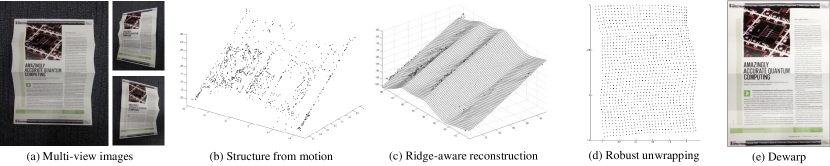
Figure 1: Our technique recovers a ridge-aware 3D reconstruction of the document surface from a sparse 3D point cloud. The final rectified image is then obtained via robust conformal mapping.

In this paper, we present a convenient method for digitally rectifying heavily curved and folded paper sheets from a few uncalibrated images captured with a hand-held camera from multiple viewpoint. Our method uses structure from motion (SfM) to recover an initial sparse 3D point cloud from the uncalibrated images. To accurately recover the dense 3D shape of paper sheet without losing high-frequency structures such as folds and creases, we develop a ridge-aware surface reconstruction method. Furthermore, to achieve robustness to outliers present in the sparse SfM 3D point cloud caused by repetitive document textures, we pose the surface reconstruction task as a robust Poisson surface reconstruction based on $\ell_{1}$ optimization. Next, to unwrap the reconstructed surface, we propose a robust conformal mapping method by incorporating ridge-awareness priors and $\ell_{1}$ optimization technique. See Fig. 1 for an overview.

The contributions of our work are threefold. First, we show how ridge-aware regularization can be used for both 3D surface reconstruction and flattening (conformal mapping) to improve accuracy. Our ridge-aware reconstruction method preserves the sharp structure of folds and creases. Ridge-awareness priors act as non-local regularizers that reduce global distortions during the surface flattening step. Second, we extend the Poisson surface reconstruction [10] and least-squares conformal mapping (LSCM) [11] algorithms by explicitly dealing with outliers using $\ell_{1}$ optimization. Finally, we describe a practical system for rectifying curved and folded documents that can be used with ordinary digital cameras.

2 Related Work

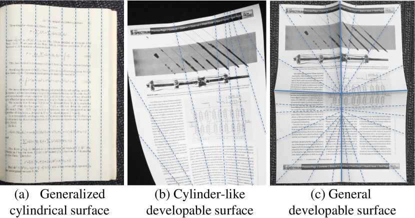
Figure 2: Developable surfaces with underlying rulers (lines with zero Gaussian curvature) and fold lines (ridges) shown as dotted and solids lines respectively. Examples of (a) smooth parallel rulers, (b) smooth rulers not parallel to each other and (c) rulers and ridges in arbitrary directions.

The topic of digital rectification of curved and folded documents has been actively studied in both the computer vision and document processing communities. It is common to model paper sheets as developable surfaces which have underlying rulers corresponding to lines with zero Gaussian curvature. Many existing methods assume generalized cylindrical surfaces where the paper is curved only in one direction and thus can be parameterized using a 1D smooth function. Such surfaces do not require an explicit parameterization of the rulers. See Fig. 2a for an example. A variety of existing techniques recover surface geometry using this assumption. Shape from shading methods were first used by Wada et al. [4], Tan et al. [12, 13], Courteille et al. [14] and Zhang et al. [5] whereas shape from boundary methods were explored by Tsoi et al. [15, 6]. Binocular stereo matching with calibrated cameras was used by Yamashita et al. [16], Koo et al. [7] and Tsoi et al. [6]. Shape from text lines is another popular method for reconstructing the document surface geometry [17, 12, 18, 19, 20, 21, 8, 22, 9, 23, 24, 25]. However, these methods assume that the document contains well-formatted printed characters.

Some recent methods relax the parallel ruler assumption (see Fig. 2b). However, the numerous parameters in these models makes the optimization quite challenging. Liang et al. [26] and Tian et al. [27] use text lines. Although these methods can handle a single input image, the strong assumptions on surface geometry, contents and illumination limit the applicability. Meng et al.designed a special calibrated active structural light device to retrieve the two parallel 1D curvatures [2], the surface can be parameterized by assuming appropriate boundary conditions and constraints on ruler orientations. Perriollat et al.[28] use sparse SfM points but assume they are reasonably dense and well distributed. Their parameterization is sensitive to noise and can be unreliable when the 3d point cloud is sparse or has varying density.

For rectification of documents with arbitrary distortion and content (Fig. 2c), other methods require specialized devices and use non-parametric approaches. Brown et al. [3] use a calibrated mirror system to obtain 3D geometry using multi-view stereo. They unwrap the reconstructed surface using constraints on elastic energy, gravity and collision. The model is not ideal for paper documents because developable surfaces are not elastic. Later, they propose using dense 3D range data [29] after which they flatten the surface using least square conformal mapping [11]. Zhang et al. [30] also use dense range scans and use rigid constraints instead of elastic constraints with the method proposed in [3]. Pilu [1] assumes that a dense 3D mesh is available and minimizes the global bending potential energy to flatten the surface. None of these existing methods are as practical and convenient as our method that only requires a hand-held camera and a few images.

3 Proposed Method

Our method has two main steps – 3D document surface reconstruction and unwrapping of the reconstructed surface. For now, we assume that a set of sparse 3D points on the surface are available. Next, we describe our new algorithms for ridge-aware surface reconstruction and robust surface unwrapping.

3.1 Ridge-aware surface reconstruction

Dense methods are favored for 3D scanning of folded and curved documents [31, 32]. This is because existing methods for surface reconstruction from sparse 3D points tend to produce excessive smoothing and fail to preserve sharp creases and folds ie. ridges on the surface. Such methods are typically also inadequate for dealing with noisy 3D points caused by repetitive textures present in documents. We address these issues by developing a robust ridge-aware surface reconstruction method for sparse 3D points. Specifically, we extend the Poisson surface reconstruction method [10] by incorporating ridge constraints and by adding robustness to outliers.

Robust Poisson surface reconstruction. We denote a set of $N$ sparse 3D points obtained from SfM as $\{\hat{x}_{n},\hat{y}_{n},\hat{z}_{n}\},n=1,2,\cdots,N$, where only 3D points triangulated from at least three images are retained. For our input images, $N$ typically lies between $700$ to $2000$. For a selected reference image (and viewpoint), we use a depth map parameterization $z(x,y)$ for the document surface. We aim to estimate depth at the mesh grid vertices $z_{i}(x_{i},y_{i})$, where $i$ is the mesh grid index, $1\leq i\leq I$. Our method computes the optimal depth values $\mathbf{z}^{*}=\left[z_{1},\ldots,z_{I}\right]^{\top}$ by solving the following optimization problem.

$$\mathbf{z}^{*}=\operatornamewithlimits{argmin}_{\mathbf{z}}E_{d}(\mathbf{z})+\lambda E_{s}(\mathbf{z}).\vspace{-6pt}$$ (1)

Here, $E_{d}$ and $E_{s}$ are the data and smoothness terms respectively and $\lambda$ is a parameter to balance the two terms. The original Poisson surface reconstruction method uses the squared $\ell_{2}$-norm for both terms. Instead, we propose using the $\ell_{1}$-norm for the data term $E_{d}$ to deal with outliers.

$$E_{d}(\mathbf{z})=\sum_{n}\|\hat{z}_{n}-z_{i}\|_{1}.\vspace{-6pt}$$ (2)

This encourages $z_{i}$ to be consistent with the observed depth $\hat{z}_{n}$ without requiring explicit knowledge about which observations are outliers. We rewrite Eq. (2) in vector form.

$$E_{d}(\mathbf{z})=\|\hat{\mathbf{z}}-{\cal P}_{\Omega}\mathbf{z}\|_{1},\vspace{-4pt}$$ (3)

where ${\cal P}_{\Omega}$ is a permutation matrix that selects and aligns observed entries $\Omega$ by ensuring correspondence between $\hat{z}_{n}$ and $z_{i}$. The smoothness term $E_{s}$ is defined using the squared Frobenius norm of the gradient of depth vector $\mathbf{z}$ along $x$ and $y$ in camera coordinates.

$$E_{s}(\mathbf{z})=\|\nabla^{2}\mathbf{z}\|_{F}^{2}=\left\|\left[\frac{\partial^{2}\mathbf{z}}{\partial x^{2}},~{}\frac{\partial^{2}\mathbf{z}}{\partial y^{2}}\right]\right\|_{F}^{2}.\vspace{-4pt}$$ (4)

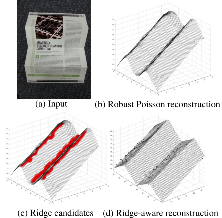
Figure 3: Example of ridge-aware 3D surface reconstruction.

By preparing a sparse derivative matrix $\mathbf{D}$ that replaces the Laplace operator $\nabla^{2}$ in a linear form,

$$\mathbf{D}=\footnotesize{\left[\begin{split}d_{i,j}&=\begin{cases}2~{}~{}&\mathrm{if}~{}~{}i=j\\ -1~{}~{}&\mathrm{if}~{}~{}z_{j}~{}\mathrm{is~{}left/right~{}to}~{}z_{i}\\ 0~{}~{}&\mathrm{otherwise}\end{cases}\\ d_{i+I,j}&=\begin{cases}2~{}~{}&\mathrm{if}~{}~{}i=j\\ -1~{}~{}&z_{j}~{}\mathrm{is~{}above/below}~{}z_{i}\\ 0~{}~{}&\mathrm{otherwise}\end{cases}\end{split}\right]_{2I\times I}},\vspace{-4pt}$$ (5)

we have a special form of the Lasso problem [33].

$$\mathbf{z}^{*}=\operatornamewithlimits{argmin}_{\mathbf{z}}\|\hat{\mathbf{z}}-{\cal P}_{\Omega}\mathbf{z}\|_{1}+\lambda\|\mathbf{D}\mathbf{z}\|_{2}^{2}.\vspace{-4pt}$$ (6)

While this problem (Eq. (6)) does not have a closed form solution, we use a variant of iteratively reweighted least squares (IRLS) [34] for deriving the solution. By rewriting the data terms in Eq. (6) as a weighted $\ell_{2}$ norm using a diagonal matrix $\mathbf{W}$ with positive values on the diagonal, we have

$$\!\!\!\mathbf{z}^{*}\!\!=\!\!\operatornamewithlimits{argmin}_{\mathbf{z}}\left(\hat{\mathbf{z}}-{\cal P}_{\Omega}\mathbf{z}\right)^{\top}\mathbf{W}^{\top}\mathbf{W}\left(\hat{\mathbf{z}}-{\cal P}_{\Omega}\mathbf{z}\right)+\lambda\mathbf{z}^{\top}\mathbf{D}^{\top}\mathbf{D}\mathbf{z}.\vspace{-4pt}$$ (7)

In contrast to Equation (6), the data term now uses $\ell_{2}$ norm instead of $\ell_{1}$ norm. We solve this problem (Equation (7)) using alternation as described next.

Step 1: Update $\mathbf{z}$

Eq. (7) can be rewritten as $\mathbf{z}^{*}=\operatornamewithlimits{argmin}_{z}\parallel\mathbf{A}\mathbf{z}-\mathbf{b}\parallel_{2}^{2}$, where $\mathbf{A}=\left[\begin{array}[]{ccc}\mathbf{W}{\cal P}_{\Omega}\\ \sqrt{\lambda}\mathbf{D}\end{array}\right]$ and $\mathbf{b}=\left[\begin{array}[]{ccc}\mathbf{W}\mathbf{\hat{z}}\\ \mathbf{0}_{2I\times 1}\end{array}\right]$ and $\mathbf{0}_{2I\times 1}$ is a zero vector of length $2I$. This is a squared $\ell_{2}$ sparse linear system. It has the closed form solution

$$\mathbf{z}^{*}=[\mathbf{A}^{\top}\mathbf{A}+\alpha\mathbf{I}]^{-1}\mathbf{A}^{\top}\mathbf{b},\vspace{-4pt}$$ (8)

where $\mathbf{I}$ is the identity matrix, $\alpha$ is a regularization parameter (we use $\alpha=1.0\text{e-}8$).

Step 2: Update $\mathbf{W}$

We initialize $\mathbf{W}$ to the identity matrix. During each iteration, each diagonal element $w_{i}$ of $\mathbf{W}$ is updated given the residual $\mathbf{r}=\mathbf{W}{\cal P}_{\Omega}\mathbf{z}^{*}-\mathbf{W}\mathbf{b}$, as follows.

$$w_{i}=\frac{1}{|r_{i}|+\epsilon},\vspace{-4pt}$$ (9)

Here, $r_{i}$ is the $i$-th element of $\mathbf{r}$ and $\epsilon$ is a small positive value (we use $\epsilon=1.0\text{e-}8$). These steps are repeated until convergence; namely, until the estimate at $t$-th iteration $\mathbf{z}^{*(t)}$ becomes similar to the previous estimate $\mathbf{z}^{*(t-1)}$, i.e., $\|\mathbf{z}^{*(t)}-\mathbf{z}^{*(t-1)}\|_{2}<1.0\text{e-}8$. Figure 3.c shows an example of the reconstructed mesh.

Ridge-aware reconstruction. Developable surfaces are ruled [35], i.e., contain straight lines on the surface as shown in Fig. 2. Our method exploits this geometric property as described in this section. Unlike existing parameterization-based methods which only handle smooth rulers, [26, 27, 2, 28], extracting arbitrary creases and ridges is more difficult when only sparse 3D points are available. We propose a sequential approach by first detecting ridges on the mesh ${\mathbf{z}^{*}}$ that was obtained using our robust Poisson reconstruction method. After selecting the ridge candidates, we instantiate additional linear ridge constraints and incorporate them into the linear system that was solved earlier. This sequential approach is quite general and avoids overfitting. It also avoids spurious ridge candidates arising due to noise.

For each point $z(x,y)$ on the mesh $\mathbf{z}^{*}$, we compute the Hessian $\mathbf{K}$ as follows.

$$\mathbf{K}(z)=\left[\begin{array}[]{ccc}\frac{\partial^{2}z}{\partial x^{2}}&\frac{\partial^{2}z}{\partial x\partial y}\\ \frac{\partial^{2}z}{\partial x\partial y}&\frac{\partial^{2}z}{\partial y^{2}}\end{array}\right].\vspace{-4pt}$$ (10)

Based on the following Eigen decomposition of $\mathbf{K}(z)$,

$$\mathbf{K}(z)=\left[\mathbf{p}_{1},\mathbf{p}_{2}\right]\left[\begin{array}[]{ccc}\kappa_{1}&0\\ 0&\kappa_{2}\end{array}\right]\left[\mathbf{p}_{1},\mathbf{p}_{2}\right]^{\top},\vspace{-4pt}$$ (11)

we obtain principal curvatures $\kappa_{1}$ and $\kappa_{2}$ ($|\kappa_{1}|\leq|\kappa_{2}|$) and the corresponding eigenvectors $\mathbf{p}_{1}$ and $\mathbf{p}_{2}$.

The value of $\kappa_{1}$ is equal to zero at all points on a developable surface. Thus, at any point $z_{i}$, a straight line along direction $\mathbf{p}_{1}$ must lie on the surface. As discussed earlier and shown in Fig. 2, the curvature along the ridge is zero while the curvature orthogonal to the ridge reaches a local extremum. We use this observation to select ridge candidates using the value of $|\kappa_{2}|$. Mesh points $z_{i}(x_{i},y_{i})$ with $|\kappa_{2}(i)|$ greater than the threshold $\kappa_{th}$ are selected as ridge candidates. (see Figure 3d for an example). The associated smoothness constraints in Eq. (4) are adjusted as follows.

$$\begin{split}\tilde{d}_{i,j}&=\varphi(\langle\mathbf{p}_{1},\mathbf{e}_{1}\rangle)d_{i,j}\\ \tilde{d}_{i+I,j}&=\varphi(\langle\mathbf{p}_{1},\mathbf{e}_{2}\rangle)d_{i+1,j},\end{split}\vspace{-4pt}$$ (12)

where $\langle~{},~{}\rangle$ is the inner product and $\mathbf{e}_{1}=[1,0]^{\top},\mathbf{e}_{2}=[0,1]^{\top}$ are orthonormal bases. $\varphi(\cdot)$ is a convex monotonic function defined as $\varphi(x)=\frac{\beta^{x^{2}}-1}{\beta-1}$, which places a greater weight $\beta\gg 1$ along the ridge and smaller weight orthogonal to it. We also consider two more directional smoothness constraints similar to those stated in Eq. (12), for the two diagonal directions $\mathbf{e}_{3}=[\frac{\sqrt{2}}{2},\frac{\sqrt{2}}{2}]^{\top}$ and $\mathbf{e}_{4}=[\frac{\sqrt{2}}{2},-\frac{\sqrt{2}}{2}]^{\top}$.

Finally, we modify $E_{s}(\mathbf{z})$ defined in Eq. (4) by adding these ridge constraints and solve a new sparse linear system (similar to the earlier one) to obtain the final reconstruction. Figure 3e shows that this method can preserve accurate folds and creases.

3.2 Surface Unwrapping

Given the 3D surface reconstruction, our next step is to unwrap the surface. We take a conformal mapping approach to this problem, amongst which, Least Squares Conformal Mapping (LSCM) [11, 29] is a suitable choice. However, it is not resilient to the presence of outliers and susceptible to global distortion which can occur due to the absence of long-range constraints. We address both these issues and extend LSCM by incorporating an appropriate robustifier as well as ridge constraints to reduce global drift.

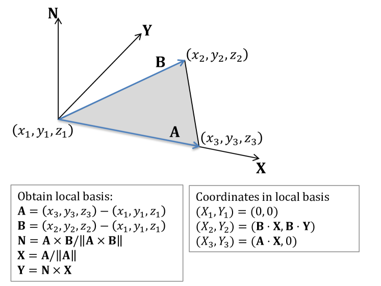
Figure 4: Vertices of a triangle in a local coordinate basis.

Conformal Mapping. For our mesh topology, each 3D point $z_{i}(x_{i},y_{i}),i=1,\dots,I$, on the grid on $\mathbf{z}$ forms two triangles, one with its upper and left neighbor, the other with its lower and right neighbor on the grid. The triangulated 3D mesh is denoted as $\{\mathbf{\cal T},\mathbf{z}\}$. A conformal map will produce an associated 2D mesh with the same connectivity but with 2D vertex positions such that the angle of all the triangles are best preserved. We denote the 2D mesh as $\{\mathbf{\cal T},\mathbf{u}\}$, where $\mathbf{u}=(u_{i},v_{i})$.

For a particular 3D triangle $t$ with vertices at $(x_{1},y_{1},z_{1})$, $(x_{2},y_{2},z_{2})$, and $(x_{3},y_{3},z_{3})$, we seek its associated 2D vertex positions ($(u_{1},v_{1})$, $(u_{2},v_{2})$ and $(u_{3},v_{3})$) under the conformal map. Using a local 2D coordinate basis for triangle $t$, the conformality constraint is captured by the following linear equations.

$$\frac{1}{S}\tiny{\left[\begin{array}[]{cccccc}\Delta X_{1}&\Delta X_{2}&\Delta X_{3}&-\Delta Y_{1}&-\Delta Y_{2}&-\Delta Y_{3}\\ \Delta Y_{1}&\Delta Y_{2}&\Delta Y_{3}&\Delta X_{1}&\Delta X_{2}&\Delta X_{3}\end{array}\right]}\mathbf{u}_{t}=\mathbf{0},\vspace{-4pt}$$ (15)

Here, $\mathbf{u}_{t}=[u_{1},u_{2},u_{3},v_{1},v_{2},v_{3}]^{\top}$, $S$ is the area of $t$, $\Delta X_{1}=(X_{3}-X_{2})$, $\Delta X_{2}=(X_{1}-X_{3})$ and $\Delta X_{3}=(X_{2}-X_{1})$ ($\Delta Y$ is similarly defined). Note that variables $(X_{1},Y_{1})$, $(X_{2},Y_{2})$, and $(X_{3},Y_{3})$ were obtained from $t$’s vertex coordinates (see Fig. 4). Putting together the constraints for all the triangles, we have the following sparse linear system.

$$\mathbf{C}\mathbf{u}=\mathbf{0}.\vspace{-6pt}$$ (16)

Using indices $i$ and $j$ to index the $I$ vertices and $J$ triangles respectively, the $2J\times 2I$ matrix $\mathbf{C}$ in Equation (16) has the following non-zero entries.

$$\begin{array}[]{cc}c_{j,i}=\frac{\Delta X}{S_{j}},&c_{j,i+I}=-\frac{\Delta Y}{S_{j}}\\ c_{j+J,i}=\frac{\Delta Y}{S_{j}},&c_{j+J,i+I}=\frac{\Delta X}{S_{j}}\end{array}\vspace{-4pt}$$ (19)

Ridge constraints. Notice that the original conformal mapping has only local constraints, which will result in global distortion, Fig. 5.f. To reduce global distortions during unwrapping, we add ridge and boundary constraints to constrain the solution further.

We take into consideration two facts. First, the ridge lines remain straight after flattening but should essentially become invisible on the flattened surface. Second, the conformal mapping constraint Eq. (15) applies to beyond triangles. In particular, it is true for three collinear points. Therefore, we propose using the collinearity property to derive non-local constraints during flattening. and add it to our conformal map estimation problem. Referring to Fig. 4, and imagine the collinear case, that is when point $(x_{2},y_{2},z_{2})$ is also lying on the $\mathbf{X}$ axis; in such case, $Y_{2}=Y_{1}=Y_{3}=0$. In addition, the area of the triangle $T$ is zero. Hence, the ridge constraints can be written in a form similar to Eq. (15).

$$\footnotesize{\left[\begin{array}[]{cccccc}\Delta X_{1}&\Delta X_{2}&\Delta X_{3}&0&0&0\\ 0&0&0&\Delta X_{1}&\Delta X_{2}&\Delta X_{3}\end{array}\right]}\mathbf{u}_{\cal R}=\mathbf{0}.\vspace{-4pt}$$ (22)

where $\mathbf{u}_{\cal R}=[u_{1},u_{2},u_{3},v_{1},v_{2},v_{3}]^{\top}$ are the targeted 2D coordinates similarly defined as $\bm{u}_{t}$. We select ridge candidates in the same way as we did earlier during reconstruction. However, this step is now more accurate because the surface is well reconstructed. For each ridge candidate (vertex), we find two farthest ridge candidates along the ridge line in opposite directions and instantiate the above mentioned constraint for the three points. We assume that the boundary of the flattened 2D document image has straight line segments (they need not be straight lines on the 3D surface). These boundary constraints can be expressed in a form similar to Eq. (22). We incorporate all ridge and boundary constraints into a system of linear equations.

$$\mathbf{R}\mathbf{u}=\mathbf{0}.\vspace{-8pt}$$ (23)

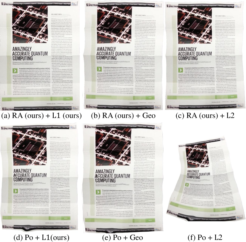
Figure 5: Rectification results from combination of methods. Acronyms RA and Po denote our ridge-aware method and Poisson reconstruction respectively. L1 denotes our $\ell_{1}$ conformal mapping method with non-local constraints; L2 indicates LSCM [29] and Geo indicates geodesic unwrapping [30]. Po + L2 produced gross failures and is thus not compared.

Robust conformal mapping. We propose using an $\ell_{1}$ norm instead of the standard squared $\ell_{2}$ norm to make conformal mapping robust to outliers. Putting together Eqs. (16) and (23) in the $\ell_{1}$ sense, we have

$$\mathbf{u}^{*}=\operatornamewithlimits{argmin}_{\mathbf{u}}\parallel\mathbf{C}\mathbf{u}\parallel_{1}+\gamma\parallel\mathbf{R}\mathbf{u}\parallel_{1},\vspace{-18pt}$$ (24)

where $\gamma$ balances the ridge and boundary constraints. To avoid the trivial solution $\mathbf{u}=0$, we fix two points of $\mathbf{u}$ to $(u_{i},v_{i})=(0,0)$ and $(u_{j},v_{j})=(0,1)$. Equation (24) is then rewritten as

$$\mathbf{u}^{*}=\operatornamewithlimits{argmin}_{\mathbf{u}}\parallel\mathbf{C}\mathbf{u}\parallel_{1}+\gamma\parallel\mathbf{R}\mathbf{u}\parallel_{1}+\theta\parallel E_{\rm{fix}}\parallel_{2}^{2},\vspace{-9pt}$$ (25)

where $E_{\rm{fix}}$ is the energy function for the two fixed points. We solve the objective function using the iterative reweighted least squares method [34]. Figure 5 shows a result from the conventional LSCM ($\ell_{2}$ method) and our proposed $\ell_{1}$ method.

3.3 Implementation details

Sparse 3D reconstruction. We recover the initial sparse 3D point cloud using SfM. While any existing SfM method is applicable, we use the popular incremental SfM technique et al. [36] in our system. We typically capture five to ten still images for each document from different viewpoints. Capturing these images or equivalently a set of burst photos or a short video clip only takes a few seconds. Figure 1a shows an input example and the corresponding reconstruction.

Image warping. After recovering the flattened mesh grid $\mathbf{u}=\{u_{i},v_{i}\}$, we unwrap the input image with the maximum document area in pixels. To obtain correspondence between the input image and $\{u_{i},v_{i}\}$, we project the 3D mesh points $\{z_{i}(x_{i},y_{i})\}$ into the image to obtain image coordinates $\{\tilde{x_{i}},\tilde{y_{i}}\}$ using the camera pose estimated using SfM. We then warp the image according to the correspondence between $\{\tilde{x_{i}},\tilde{y_{i}}\}$ and $\{u_{i},v_{i}\}$ with bilinear interpolation.

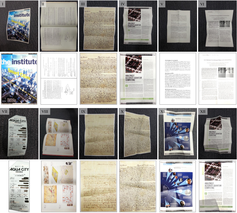
Figure 6: [Our results] Original images are shown in rows 1 and 3 and our rectification results are shown in rows 2 and 4.

4 Experiments

We perform qualitative and quantitative evaluation on a wide variety of input documents. The first set of experiments show that our method can handle different paper types, document content and various types of folds and creases. Next, we report a quantitative evaluation based on known ground truth using local and global metrics where we demonstrate the superior performance and advantages of our method over existing methods [29, 30, 28]. In all the experiments, we set parameters as follows: $\lambda=1\text{e-}5,\beta=40,$ $\gamma=1e3$, $\theta=1e2$ and $\kappa_{th}=0.006$. Our method is insensitive to these parameters. Varying $\lambda,\gamma,\theta$ by factors of 0.1 – 1.0 or varying $\beta$ or $\kappa_{th}$ by 50% from these settings did not change the result significantly.

4.1 Test Data

The first six out of the 12 test sequences (I – VI) contain documents with no fold lines, one fold line, two to three parallel fold lines, and two to three crossing fold lines respectively. The other six sequences (VII – XII) contain documents with an increasing number of fold lines. Irregular fold lines were intentionally added to make the rectification more challenging. All documents were either placed on a planar or curved background surface. Sequence VII contains a shopping receipt on a paper roll whereas II and VIII contain pages from a book. Sequences III, IV, IX and X contain letters folded within envelopes. Sequence V, VI, XI and XII contain examples of documents folded inside a purse or notebook. The input images as well as the results from our method are shown in Fig. 6. Our method does not rely on the content, formatting, layout or color of the document. Thus, it is generally applicable as long as a sufficient number of sparse keypoints in the input images are available for SfM.

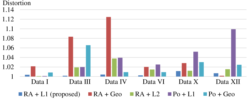
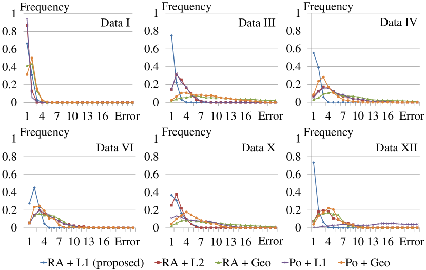
Global distortion evaluation metric Local distortion evaluation metric

Figure 7: Distortion metrics for datasets shown in Fig. 6. Abbreviations are consistent with Fig. 5 and the text.

4.2 Quantitative Evaluation Metrics

We quantitatively evaluate the global and local distortion between the ground truth digital image and our rectified result using local and global metrics. The digital version of six out of the 12 test documents were available. We treat those images as ground truth and resize them by setting their height to 1000 pixels.

Global distortion metric. We first register the rectified image to the ground truth by estimating a global affine transform $T$ estimated using SIFT keypoint correspondences in these images [37].

$$\mathbf{T}=\left[\small\begin{array}[]{ccc}a_{1}&a_{2}&t_{1}\\ a_{3}&a_{4}&t_{2}\\ 0&0&s\end{array}\right],\vspace{-8pt}$$ (29)

This is achieved by minimizing the squared error.

$$\mathbf{T}^{*}=\operatornamewithlimits{argmin}_{\mathbf{T}}\parallel\mathbf{T}\mathbf{p}-\mathbf{\hat{p}}\parallel_{2}^{2}.\vspace{-8pt}$$ (30)

where, $\mathbf{p}$ and $\mathbf{\hat{p}}$ denote corresponding 2D keypoint positions using homogenous coordinates. We compute the global distortion metric $\mathcal{G}$ as follows.

$$\begin{split}G&=(a_{1}a_{4}-a_{2}a_{3})/s^{2}\\ \mathcal{G}&=\max{(G,1/G}).\end{split}\vspace{-6pt}$$ (31)

A perfect result has $\mathcal{G}=1$; and larger values indicate more distortion (see comparative results in Fig. 7).

Local distortion metric. We compute the local metric by performing dense image registration using SIFT-flow [38] between the rectified image and the ground truth image. The frequency distribution of local displacements are shown in lower figure in Fig. 7 and compared with existing methods. We found dense registration to be more useful for an unbiased evaluation than sparse SIFT keypoint-based registration because sparse methods are more likely to ignore many matches if the result contains large deformations.

4.3 Comparison with existing methods

We first compare with three methods [28, 29, 30] on various real images and then use synthetically generated data to further compare with the methods designed for dense 3D point data  [29, 30].

Perriollat et al. [28]. Their method explicitly parameterizes smooth rulers but cannot handle our document images with creases and folds. Our method works fine on their dataset and produces a more accurate result than the one obtained by running their code (see Fig. 8). Although our result has minor artifacts due to self-occlusion and fore-shortening, the flattening result is quite accurate.

Brown et al. [29], Zhang et al. [30]. We compare to both methods using our sequences where ground truth is available (Fig. 6). Since they require 3D range data, we use our reconstructed surface as their input and compare the surface flattening quality. We also compare our ridge-aware reconstruction to the standard Poisson reconstruction method. As shown in Fig. 7, the global and local distortion metrics introduced earlier are used in the evaluation. Our method has higher accuracy in terms of both metrics. Results from various methods have been compared in Fig. 5.

Evaluation on synthetic data. We compared our method with [29, 30] on synthetically generated dense 3D points because these methods require dense 3D points. We vary the point cloud size from 2K to 300K (common in 3D range data) and inject varying levels of Gaussian noise. The results from the three methods are compared in Figure 9. These experiments show that with low noise and high point density, all three methods are comparable in accuracy. However, when the points are sparser or when the noise level is higher, our method is more accurate than prior methods [29, 30].

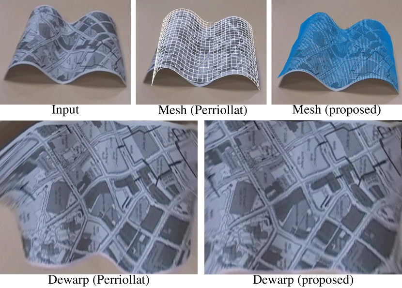
Figure 8: Visual comparison with cylindrical like surface based method which uses SfM as input [28].

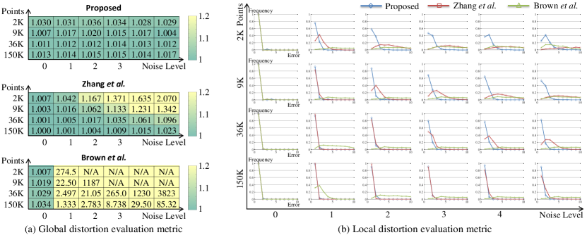
Figure 9: Comparison of the global distortion metric between our method (top) and Zhang et al. [30] and Brown et al.[29] with varying point density and noise. Here lower values indicate higher accuracy. (b) Frequency distribution of local distortion metrics for the associated experiments. Our method is more accurate when input point are sparser or have more noise.

5 Conclusion and Future Work

In this paper, we propose a method for automatically rectifying curved or folded paper sheets from a small number of images captured from different viewpoints. We use SfM to obtain sparse 3D points from images and propose ridge-aware surface reconstruction method which utilizes the geometric property of developable surface for accurate and dense 3D reconstruction of paper sheets. We also robustify the algorithms using $\ell_{1}$ optimization techniques. After recovering surface geometry, we unwrap the surface by adopting conformal mapping with both local and non-local constraints in a robust estimation framework. In the future we will address the correction of photometric inconsistencies in the document image caused by shading under scene illumination.

References

- [1] M. Pilu, “Undoing paper curl distortion using applicable surfaces,” in CVPR. IEEE, 2001.
- [2] G. Meng, Y. Wang, S. Qu, S. Xiang, and C. Pan, “Active flattening of curved document images via two structured beams,” in CVPR. IEEE, 2014.
- [3] M. S. Brown and W. B. Seales, “Image restoration of arbitrarily warped documents,” TPAMI, vol. 26, no. 10, pp. 1295–1306, 2004.
- [4] T. Wada, H. Ukida, and T. Matsuyama, “Shape from shading with interreflections under a proximal light source: Distortion-free copying of an unfolded book,” IJCV, vol. 24, no. 2, pp. 125–135, 1997.
- [5] L. Zhang, A. M. Yip, M. S. Brown, and C. L. Tan, “A unified framework for document restoration using inpainting and shape-from-shading,” Pattern Recognition, vol. 42, no. 11, pp. 2961–2978, 2009.
- [6] Y.-C. Tsoi and M. S. Brown, “Multi-view document rectification using boundary,” in CVPR. IEEE, 2007.
- [7] H. I. Koo, J. Kim, and N. I. Cho, “Composition of a dewarped and enhanced document image from two view images,” TIP, vol. 18, no. 7, pp. 1551–1562, 2009.
- [8] N. Stamatopoulos, B. Gatos, I. Pratikakis, and S. J. Perantonis, “Goal-oriented rectification of camera-based document images,” TIP, vol. 20, no. 4, pp. 910–920, 2011.
- [9] Z. Zhang, X. Liang, and Y. Ma, “Unwrapping low-rank textures on generalized cylindrical surfaces,” in ICCV. IEEE, 2011, pp. 1347–1354.
- [10] M. Kazhdan, M. Bolitho, and H. Hoppe, “Poisson surface reconstruction,” in Fourth Eurographics symposium on Geometry processing, 2006.
- [11] B. Lévy, S. Petitjean, N. Ray, and J. Maillot, “Least squares conformal maps for automatic texture atlas generation,” in ACM TOG, vol. 21. ACM, 2002, pp. 362–371.
- [12] Z. Zhang, C. Lim, and L. Fan, “Estimation of 3d shape of warped document surface for image restoration,” in ICPR, 2004.
- [13] C. L. Tan, L. Zhang, Z. Zhang, and T. Xia, “Restoring warped document images through 3d shape modeling,” TPAMI, vol. 28, no. 2, pp. 195–208, 2006.
- [14] F. Courteille, A. Crouzil, J.-D. Durou, and P. Gurdjos, “Shape from shading for the digitization of curved documents,” Machine Vision and Applications, vol. 18, no. 5, pp. 301–316, 2007.
- [15] Y.-C. Tsoi and M. S. Brown, “Geometric and shading correction for images of printed materials: a unified approach using boundary,” in CVPR. IEEE Computer Society, 2004.
- [16] A. Yamashita, A. Kawarago, T. Kaneko, and K. T. Miura, “Shape reconstruction and image restoration for non-flat surfaces of documents with a stereo vision system,” in ICPR. IEEE, 2004.
- [17] H. Cao, X. Ding, and C. Liu, “A cylindrical surface model to rectify the bound document image,” in ICCV, 2003.
- [18] H. Ezaki, S. Uchida, A. Asano, and H. Sakoe, “Dewarping of document image by global optimization,” in ICDAR. IEEE, 2005.
- [19] A. Ulges, C. H. Lampert, and T. M. Breuel, “Document image dewarping using robust estimation of curled text lines,” in ICDAR. IEEE, 2005.
- [20] S. Lu, B. M. Chen, and C. C. Ko, “A partition approach for the restoration of camera images of planar and curled document,” Image and Vision Computing, vol. 24, no. 8, pp. 837–848, 2006.
- [21] B. Fu, M. Wu, R. Li, W. Li, Z. Xu, and C. Yang, “A model-based book dewarping method using text line detection,” in 2nd Int. Workshop on Camera Based Document Analysis and Recognitionl, 2007.
- [22] G. Meng, C. Pan, S. Xiang, J. Duan, and N. Zheng, “Metric rectification of curved document images,” TPAMI, vol. 34, no. 4, pp. 707–722, 2012.
- [23] C. Liu, Y. Zhang, B. Wang, and X. Ding, “Restoring camera-captured distorted document images,” IJDAR, vol. 18, no. 2, pp. 111–124, 2014.
- [24] B. S. Kim, H. I. Koo, and N. I. Cho, “Document dewarping via text-line based optimization,” Pattern Recognition, 2015.
- [25] D. Salvi, K. Zheng, Y. Zhou, and S. Wang, “Distance transform based active contour approach for document image rectification,” in WACV. IEEE, 2015.
- [26] J. Liang, D. DeMenthon, and D. Doermann, “Geometric rectification of camera-captured document images,” TPAMI, vol. 30, no. 4, pp. 591–605, 2008.
- [27] Y. Tian and S. G. Narasimhan, “Rectification and 3d reconstruction of curved document images,” in CVPR. IEEE, 2011.
- [28] M. Perriollat and A. Bartoli, “A computational model of bounded developable surfaces with application to image-based three-dimensional reconstruction,” Computer Animation and Virtual Worlds, vol. 24, no. 5, pp. 459–476, 2013.
- [29] M. S. Brown, M. Sun, R. Yang, L. Yun, and W. B. Seales, “Restoring 2d content from distorted documents,” TPAMI, vol. 29, no. 11, pp. 1904–1916, 2007.
- [30] L. Zhang, Y. Zhang, and C. L. Tan, “An improved physically-based method for geometric restoration of distorted document images,” TPAMI, vol. 30, no. 4, pp. 728–734, 2008.
- [31] H. Avron, A. Sharf, C. Greif, and D. Cohen-Or, “ℓ 1-sparse reconstruction of sharp point set surfaces,” ACM TOG, 2010.
- [32] A. C. Öztireli, G. Guennebaud, and M. Gross, “Feature preserving point set surfaces based on non-linear kernel regression,” in Computer Graphics Forum, vol. 28, no. 2. Wiley Online Library, 2009, pp. 493–501.
- [33] R. Tibshirani, “Regression shrinkage and selection via the lasso,” Journal of the Royal Statistical Society. Series B (Methodological), pp. 267–288, 1996.
- [34] E. J. Candes, M. B. Wakin, and S. P. Boyd, “Enhancing sparsity by reweighted minimization,” Journal of Fourier analysis and applications, vol. 14, no. 5-6, pp. 877–905, 2008.
- [35] E. Portnoy, “Developable surfaces in hyperbolic space,” Pacific Journal of Mathematics, vol. 57, no. 1, pp. 281–288, 1975.
- [36] R. I. Hartley and A. Zisserman, Multiple View Geometry in Computer Vision, 2nd ed. Cambridge University Press, ISBN: 0521540518, 2004.
- [37] D. G. Lowe, “Distinctive image features from scale-invariant keypoints,” IJCV, vol. 60, no. 2, pp. 91–110, 2004.
- [38] C. Liu, J. Yuen, A. Torralba, J. Sivic, and W. T. Freeman, “Sift flow: Dense correspondence across different scenes,” in ECCV, 2008.