Highly Parallel Demagnetization Field Calculation Using the Fast Multipole Method on Tetrahedral Meshes with Continuous Sources

Abstract

The long-range magnetic field is the most time-consuming part in micromagnetic simulations. Improvements both on a numerical and computational basis can relief problems related to this bottleneck. This work presents an efficient implementation of the Fast Multipole Method [FMM] for the magnetic scalar potential as used in micromagnetics. We assume linearly magnetized tetrahedral sources, treat the near field directly and use analytical integration on the multipole expansion in the far field. This approach tackles important issues like the vectorial and continuous nature of the magnetic field. By using FMM the calculations scale linearly in time and memory.

1 Introduction

Micromagnetic algorithms are an important tool for the simulation of ferromagnetic materials used in electric motors, storage systems and magnetic sensors. In micromagnetic simulations the demagnetization field is the most time-consuming part. Many different algorithms for solving the problem exist, e.g. [12, 5, 6, 18, 3, 15, 4, 16, 1, 11]. Direct solutions compute all pair-wise interactions and hence they scale with $\mathcal{O}\bigl{(}N^{2}\bigr{)}$ operations, where $N$ denotes the number of interaction partners.

Modern Finite Element Method (FEM) implementations[7, 1] have linear scaling for the Poisson equation only for closed boundary conditions when a multigrid preconditioner is used[20]. The demagnetization potential has open boundary conditions defined at infinity. For the computation of the potential at the boundary, hybrid FEM/BEM[12] (Finite Element Method with Boundary Element Method Coupling) and the shell transformation approach [5] add an additional complexity of $\mathcal{O}\bigl{(}M^{2}\bigr{)}$, where $M$ denotes the number of surface triangles. This can be further reduced to $\mathcal{O}\bigl{(}M\log(M)\bigr{)}$ by the use of $\mathcal{H}$-matrix approximation [6, 18, 15] or fast summation techniques utilizing non-uniform fast Fourier transform (NUFFT) [10].

The Fast Multipole Method (FMM) was originally invented by Greengard and Rokhlin[14] for particle simulations. The version presented in this paper is an extension to the class of Fast Multipole Codes [8, 19, 22]. This version is based on the direct evaluation of volume integrals, putting it in a category with nonuniform grid ([16]), Fast Fourier Transform [FFT] methods ([17, 1]) and Tensor Grid methods ([11]). A useful comparison of existing codes is given in the review [2]. The basis of the presented approach is a spatial discretization of the analytical expression of the integral representation of the magnetic scalar potential

$$u(\mathbf{r})=\frac{1}{4\pi}\int_{\Omega}\mathbf{M}(\mathbf{r^{\prime}})\cdot\nabla^{\prime}\Big{(}\frac{1}{|\mathbf{r}-\mathbf{r}^{\prime}|}\Big{)}\,\text{d}\mathbf{r}^{\prime}$$ (1)

$$\approx\frac{1}{4\pi}\sum_{j=1}^{M}\int_{\Omega_{j}}\mathbf{M}_{j}(\mathbf{r}^{\prime})\cdot\nabla^{\prime}\Big{(}\frac{1}{|\mathbf{r}-\mathbf{r}^{\prime}|}\Big{)}\,\text{d}\mathbf{r}^{\prime},$$ (2)

where the $M$ subvolumes $\Omega_{j}$ are tetrahedrons wherein the magnetization $\mathbf{M}_{j}$ is assumed to be linear (i.e.affine basis functions). The FMM approach in this work approximates (2) by treating the near field both directly and analytically and the far field by (exact) numerical integration of a multipole expansion of the integrated convolution kernels.

Among the above mentioned methods only the FEM/BEM approach and a non-uniform FFT[10] approach are suited for irregular grids, but FMM is expected to scale better to many processors because of its small memory footprint. Some implementations of current micromagnetic FMM codes [25, 4] only support homogeneously magnetized regular grids. The hereby presented method works on linearly magnetized tetrahedrons, making it a suitable alternative to FEM codes on irregular grids. However, the tetrahedral nature of the sources complicates the FMM procedure by demanding more elaborate approaches for the direct interaction (see section 2.1) and multipole expansion (see section 2.2). This work manages to preserve the optimal linear scaling of FMM codes with good performance even for small problems (see fig. 6) while using low storage compared to most other algorithms. The storage requirements are particularly important for large problems as well.

The paper is divided as follows. We present the relevant mathematical and algorithmic preliminaries of the method in the next section. Implementation details are given in section 3. In the numerics section (section 4) we compare the results for the problem of a homogeneously magnetized box to the analytic solution. Details related to analytical integration over tetrahedrons are stated in appendix A.

2 Fast Multipole Expansion [FMM]

The fast multipole method is a method for computing equations of the form

$$u_{i}=\sum_{j}D_{\mathbf{n}}\left(s_{j}-t_{i}\right)Q_{j},$$

where $u_{i}$ is the potential at the $i$th evaluation position, $D_{\mathbf{n}}\left(\mathbf{r}\right)$ is a so called kernel function, $t_{i}$ are called target-, $s_{j}$ source-points and $Q_{j}$ magnetizations or charges. For a dense kernel, this computation would need $\mathcal{O}\bigl{(}N^{2}\bigr{)}$ operations, compared to the $\mathcal{O}\bigl{(}N\bigr{)}$ for the FMM. As pointed out in [3], the key features of the FMM are:

• A specified acceptable accuracy of computation $\epsilon$ (in this case a flexible Multipole Acceptance Criterion for adjusting speed vs. accuracy; see section 3.2 and [22])

• A hierarchical division of space into source clusters (octree)

• A multipole expansion of the kernel $D_{\mathbf{n}}\left(\mathbf{r}\right)$

• (for improved performance) A method for calculating the local expansion from the far-field expansion [21]

A sketch of the the FMM algorithm is shown in fig. 1. It involves either the direct computation of the interaction of two vertices (P2P … Point to Point), or the following 5 steps:

1. Multipole expansion of the source vertex into the leave cell (P2M … Point to Multipole)

2. Collection of smaller cell multipole moments into combined multipole moments of the parent cell (M2M … Multipole to Multipole)

3. Local expansion of remote multipole moments (M2L … Multipole to Local)

4. Down conversion of local expansion coefficients to the descendant cells. (L2L … Local to Local)

5. Evaluation of the local expansion at the target vertex. (L2P … Local to Point)

where steps 2 and 4 can be done as many times as necessary.

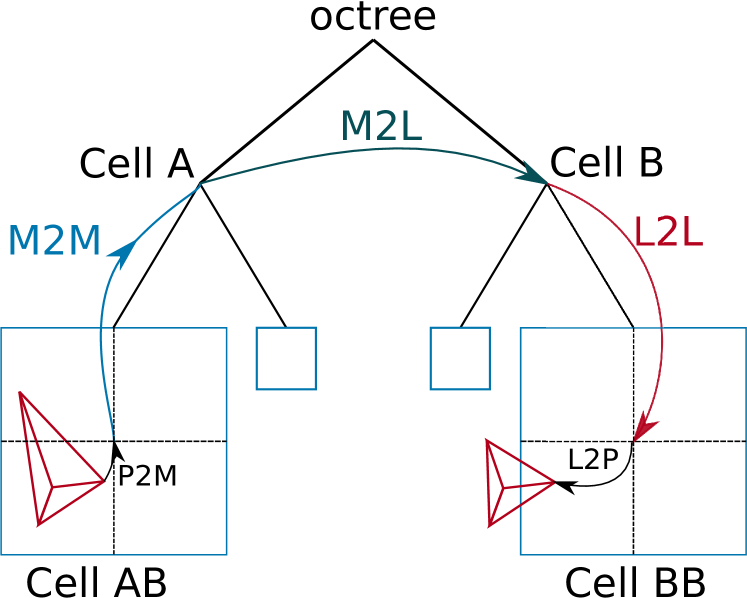
Figure 1: Overview of the FMM algorithm showing the involved operations and multipole transitions. P … Point (vertex, source or target), M … Multipole expansion of source, L … Local expansion around target cell

2.1 Direct Vertex Interaction

Each tetrahedron in the mesh is split into four tetrahedral hat functions. These hat functions are then identified with their vertices. The integration from one vertex $v_{1}$ to another vertex $v_{2}$ is then carried out by integrating over all hat functions that are non-zero at $v_{1}$. This leads to the integration shown in eq. 2. The integral (solved in the sections below) results in a vector that describes the interaction from one vertex to another. For a similar approach consult [13]. In this method, targets are treated as simple vertices. A recently published method for integrating the interaction between two polyhedrons exists[9].

2.1.1 Tetrahedron Integration Overview

Integration of the kernel function over any tetrahedral domain can be decomposed to four integrals with the target point replacing one source vertex for each vertex[13]. A two-dimensional integral decomposition can be seen in fig. 2. This step simplifies the problem into four integrations of tetrahedrons with an $\mathbf{r}$ at a corner vertex.

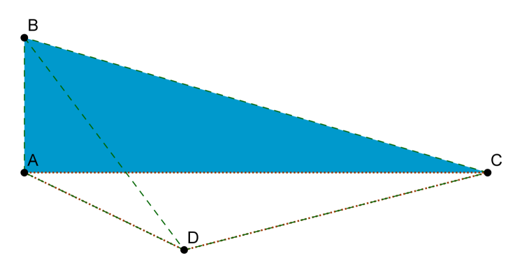
Figure 2: Decomposition of the source triangle integration (ABC; blue triangle) into three new triangles with the target (D) as vertex. The integrals described by the triangles (ABD, BCD) are added and the integral bounded by triangle (ACD) is subtracted.

Before integrating the tetrahedrons the problem is rototranslated into a new frame of reference sketched in fig. 3. The target point $v_{1}$ is set into the z-axis. The other vertices are set into the xy-plane and the source vertices $v_{2}$ and $v_{3}$ are aligned parallel to the x-axis.

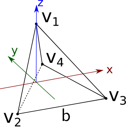
Figure 3: The rototranslated frame of reference for tetrahedron integration. With $x_{1}=y_{1}=0$, $z_{2}=z_{3}=z_{4}=0$ and $y_{2}=y_{3}$

2.1.2 Source Magnetization

The integrals can be solved for a general linear magnetization. To this end, the magnetization $\mathbf{M}(\mathbf{r^{\prime}})$ is split into a geometric part describing the linear change of the field and a value part describing the magnetization at each vertex. The hat functions set all but one source vertex to zero. Giving at most two nonzero magnetized vertices, namely the source vertex $v_{1}$ and the target vertex $v_{4}$. Without loss of generality the system of linear equations for the x-component of the field is:

$$\mathbf{M}_{\hat{x}}(x,y,z)=a_{1}+a_{2}x+a_{3}y+a_{4}z=a_{\hat{x}}\cdot{(1,x,y,z)}^{T}$$

$$\mathbf{M}_{x}\left(v_{1}=(0,0,h=1)\right) =M_{t}$$

$$\mathbf{M}_{x}\left(v_{2}=(x_{2},y_{2},0)\right) =0$$

$$\mathbf{M}_{x}\left(v_{3}=(x_{2},y_{3},0)\right) =0$$

$$\mathbf{M}_{x}\left(v_{4}=(x_{4},y_{4},0)\right) =M_{s}$$

where $M_{t}$ is the linear source field evaluated at the target vertex. And $M_{s}$ is the magnetization of the source vertex, which can be expressed in matrix form as

$$\begin{pmatrix}1&0&0&1\\ 1&x_{2}&y_{2}&0\\ 1&x_{2}&y_{3}&0\\ 1&x_{4}&y_{4}&0\end{pmatrix}\cdot\begin{pmatrix}a_{1}\\ a_{2}\\ a_{3}\\ a_{4}\end{pmatrix}=\begin{pmatrix}M_{t}\\ 0\\ 0\\ M_{s}\end{pmatrix}$$

solving to:

$$a_{\hat{x}}=\frac{1}{bs}\begin{pmatrix}M_{s}(x_{2}-x_{3})y_{2}\\ 0\\ M_{s}(x_{3}-x_{2})\\ \left(M_{s}(x_{3}-x_{2})+M_{t}(x_{3}-x_{2})(y_{4}-y_{2})\right)\end{pmatrix}$$

with $b=x_{3}-x_{2}$ and $s=y_{4}-y_{2}$

2.1.3 Tetrahedron Corner Integration

The rototranslated tetrahedron integrals are all singular but can be transformed into regular integrals by following nonlinear transformation (see also [13]):

$$x\rightarrow x_{t}(1-\lambda);y\rightarrow y_{t}(1-\lambda);\frac{z}{h}\rightarrow\lambda$$

The transformed integral creates a prism which can be integrated in $\lambda$-direction leading to following triangle integration:

$$u(\mathbf{r}) =\frac{1}{4\pi}\int_{\Omega}\mathbf{M}(\mathbf{r^{\prime}})\cdot\mathbf{\nabla}_{\!s}\frac{1}{|\mathbf{r}_{t}-\mathbf{r}_{s}|}\mathrm{d}\mathbf{r}^{\prime}$$ (3)

$$=\frac{1}{4\pi}\mathbf{a}\int_{T}\frac{x_{t}\hat{x}+y_{t}\hat{y}+h\hat{z}}{{\left(x_{t}^{2}+y_{t}^{2}+h^{2}\right)}^{\frac{3}{2}}}\begin{pmatrix}1\\ x_{t}=0\\ y_{t}\\ 1\end{pmatrix}\mathrm{d}x_{t}\mathrm{d}y_{t}$$

Note that $\mathbf{a}$ is a $3\times 4$ matrix contracting with $\hat{x},\hat{y},\hat{z}$ and ${(1,0,y_{t},1)}^{T}$.

The triangle integration boundaries have been set to:

• x-integration first ($\int_{T}\mathrm{d}x_{t}\mathrm{d}y_{t}=\int_{y-}^{y+}\int_{x-}^{x+}\mathrm{d}x_{t}\mathrm{d}y_{t}$):

  $$x_{-}=\frac{x_{1}-x_{2}}{y_{1}-y_{2}}(y-y_{2})+x_{2};\;x_{+}=\frac{x_{1}-x_{3}}{y_{1}-y_{2}}(y-y_{2})+x_{3}$$

  $$y_{-}=y_{2};\;y_{+}=y_{3}$$

• y-integration first ($\int_{T}\mathrm{d}y_{t}\mathrm{d}x_{t}=\int_{x-1}^{x+1}\int_{y-}^{y+}\mathrm{d}y_{t}\mathrm{d}x_{t}+\int_{x-2}^{x+2}\int_{y-}^{y+}\mathrm{d}y_{t}\mathrm{d}x_{t}$):

  $$y_{y-}=\frac{y_{1}-y_{2}}{x_{1}-x_{2}}(x-x_{2})+y_{2};\;y_{y+}=\frac{y_{1}-y_{2}}{x_{1}-x_{3}}(x-x_{1})+y_{1}$$

  $$x_{y-1}=x_{1};\;x_{y+1}=x_{2}$$

  $$x_{y-2}=x_{2};\;x_{y+2}=x_{3}$$

The resulting triangle integrals from eq. 3 are given in appendix A.

2.2 Source Expansion

For continuous sources an integral expression (in our case eq. 2) must be expanded. To this end the Coulomb kernel $1/|\mathbf{r}-\mathbf{r}^{\prime}|$ is expanded as a Taylor polynomial of order $p$ in terms of $\mathbf{r}^{\prime}$ around the origin (Cartesian multipole expansion)

$$\frac{1}{|\mathbf{r}-\mathbf{r}^{\prime}|}=\sum_{|\mathbf{n}|\leq p}\frac{1}{\mathbf{n}!}\,\Big{(}\frac{\partial^{\mathbf{n}}}{\partial{(-\mathbf{r})}^{\mathbf{n}}}\,\frac{1}{|\mathbf{r}|}\Big{)}{\mathbf{r}^{\prime}}^{\mathbf{n}}+\mathcal{O}(\tfrac{|\mathbf{r}^{\prime}|^{p+1}}{|\mathbf{r}|^{p+2}}).$$ (4)

where $\mathbf{n}={n_{x},n_{y},n_{z}}$ being a multi-index, $\mathbf{n}!=n_{x}!n_{y}!n_{z}!$, $|\mathbf{n}|=n_{x}+n_{y}+n_{z}$ and $\mathbf{r}^{\prime\mathbf{n}}=x^{\prime n_{x}}y^{\prime n_{y}}z^{\prime n_{z}}$. From a source point (or field point, resp.) perspective the truncation error is proportional to ${(\alpha/2)}^{p+1}$ where $\alpha$ is the opening angle $2r/d$ with $r$ being the diameter of source (or field) cell and $d$ the distance between centers [21]. Plugging the expansion into the expression for the $j$-th volume source (eq. 2) yields

$$\int_{\Omega_{j}}\mathbf{M}_{j}(\mathbf{r}^{\prime})\cdot\nabla^{\prime}\Big{(}\frac{1}{|\mathbf{r}-\mathbf{r}^{\prime}|}\Big{)}\,\text{d}\mathbf{r}^{\prime}=\sum_{|\mathbf{n}|\leq p}\frac{1}{\mathbf{n}!}\Big{(}\frac{\partial^{\mathbf{n}}}{\partial{(-\mathbf{r})}^{\mathbf{n}}}\frac{1}{|\mathbf{r}|}\Big{)}\int_{\Omega_{j}}\mathbf{M}_{j}(\mathbf{r}^{\prime})\cdot\nabla^{\prime}\mathbf{r}^{\prime\mathbf{n}}\,\text{d}\mathbf{r}^{\prime},$$ (5)

resulting in the following expansion coefficients:

$$Q_{\mathbf{n};j}=\int_{\Omega_{j}}\mathbf{M}_{j}(\mathbf{r}^{\prime})\cdot\nabla^{\prime}\mathbf{r}^{\prime\mathbf{n}}\,\text{d}\mathbf{r}^{\prime}.$$ (6)

The expansion coefficients can be calculated exactly using a quadrature rule of order $M=|\mathbf{n}|+1$ because of the polynomial nature of the integrand, i.e.

$$\int_{\Omega_{j}}f(r)\mathrm{d}^{3}r=|\Omega_{j}|\sum_{i=1}^{M}f(p_{i})w_{i},$$

using the volume of the tetrahedron $|\Omega_{j}|$ and the quadrature points $p_{i}$ with associated weights $w_{i}$ from [24].

2.3 Local Expansion

In the target octree-cell the potential $u(\mathbf{r})$ is approximated by a power series

$$u(\mathbf{r})=\sum_{\mathbf{n}}\frac{1}{\mathbf{n}!}L_{\Omega,n}r^{n}$$

again using $\mathbf{n}$ as a multi-index (see section 2.2). This gives the local expansion coefficients of

$$L_{\Omega,n}=\left(\frac{\partial^{\mathbf{n}}}{\partial\mathbf{r}^{\mathbf{n}}}u(\mathbf{r})\right)\bigg{|}_{\mathbf{r}=r_{\Omega}}.$$

The local expansion coefficients $L_{\Omega,n}$ can be computed recursively (see [21]).

3 Implementation

3.1 Hierarchical Space Division

The key to the good scalability of the algorithm is the hierarchical space division. In three dimensions a cubic box enclosing the investigated space is successively divided into octrees creating smaller and smaller cubes of space (see fig. 5). The smallest (leaf) cells contain the vertex points of the mesh. These vertices are in turn connected to linear hat functions defined by the adjacent tetrahedrons creating the irregular mesh.

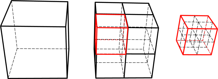
Figure 4: An octree is the successive subdivision of space into 8 smaller cubes.

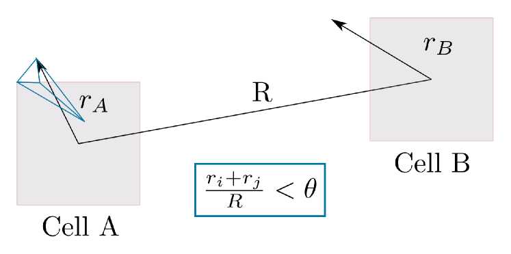
Figure 5: Multipole Acceptance Criterion: $r_{A}$ and $r_{B}$ are the radii of the remotest directly connected vertices, $R$ is the cell distance and $\theta$ the MAC parameter.

3.2 Multipole Acceptance Criterion [MAC]

The MAC is used to determine whether direct integration or multipole expansion is used for two interaction partners. The MAC is fulfilled when the combined radii are smaller than the interaction partners’ distance by a factor of $\theta$ (see fig. 5). In this case expansion is used, otherwise direct calculation. The cell radius is the distance between the cell center and the most remote vertex directly connected to the cell. A vertex is directly connected if it shares a tetrahedron with a vertex residing inside the cell. It is not the size of the cell itself.

3.3 Dual Tree Traversal

The dual tree traversal moves down the source and target tree simultaneously using the MAC to decide whether to do a multipole to local expansion (M2L) or move down a level in the larger tree and repeat the process for the newly created cell pairs. When both trees are at the leaf level a direct computation of the potential is done. The method and pseudocode for the dual tree traversal is reprinted from [22] in LABEL:lst:dtt and LABEL:lst:interact.

Listing 1: EvaluateDualTreecode()

⬇

push pair of root cells (A,B) to stack

while stack is not empty do

pop stack to get (A,B)

if target cell is larger then source cell then

for all children a of target cell A do

Interact{(a,B)}

end for

else

for all children b of source cell B do

Interact{(A,b)}

end for

end if

end while

Listing 2: Interact(A,B)

⬇

if A and B are both leafs then

call P2P kernel

else

if A and B satisfy MAC then

call M2L kernel

else

push pair (A,B) to stack

end if

end if

3.4 Storage Requirements

The algorithmic storage required is mainly composed of tree information, direct interaction coefficients, multipole coefficients, sources and targets. Obviously the source and target information scales linearly with the number of sources and targets. The direct integration coefficients stored are mainly a near field component; they scale linearly. The number of multipole and local coefficients also scales linearly but the proof is a bit more nuanced. Consider a tree with N vertices. The number of octree levels is equal to $\log_{8}(N/a)$ where $a$ is the number of vertices per leaf cell. The number of nodes per level $L$ is $8^{L}$ giving a total of

$$\sum_{n=1}^{\log_{8}(N)}8^{n}=\frac{1-8^{\log_{8}(N/8)+1}}{1-8}=\frac{N-1}{7}=O(N)$$

levels. Each level must store $p(p+1)(p+2)/6$ local and multipole coefficients. Which means it scales cubic in the multipole order. Summarizing, it can be said that the storage scales linearly in the number of sources and targets, but with cubic dependence on the multipole order $p$.

4 Numerics

This section compares the computational results of eq. 2 in an applied physical context. The near-field (P2P) evaluation described in section 2.1 was verified with randomly magnetized and randomly generated tetrahedra via numeric integration, leading to an error in the order of the numeric accuracy of the quadrature.

4.1 Comparison with FEM solvers

The present work implemented two implementations of the FMM for the use on tetrahedral grids. One for linearly magnetized meshes (Tet FMM) and another for point-like dipole clouds (Mag FMM). Focus was placed on speed and scaling. It shows that FMM is a fast usable algorithm for solving the stray-field problem which can be integrated in existing micromagnetic codes. Applications for the point-like source FMM include atomistic simulations on many cores.

Simulations on homogeneously magnetized regular boxes have been done on a modified version of the ExaFMM[22] software to determine accuracy and speed of the produced code. The speed of these simulations was compared to an optimized Finite Element Method [FEM] simulation in fig. 6.

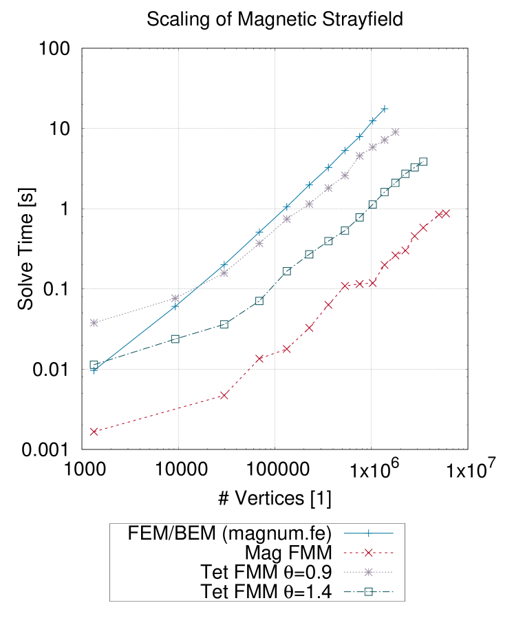
Figure 6: This plot compares the runtime of a fast FEM code (magnum.fe) to the run-time of a simple dipole FMM (Mag FMM) code and the improved FMM (Tet FMM) code with direct near-field interaction and a MAC of 0.3 (see section 3.2). Each simulation was done on one node with 16 cores.

The parameters used for the Tet FMM code were a MAC of $\theta=0.8$ and $\theta=1.4$ and a maximum multipole order of $O=4$. The parameters used for the Mag FMM code were $\theta=0.3$ and $O=4$. Mass lumping was used for the computation of the B-field and the energy.

Figure 8 shows a performance comparison of the tested methods. The Tet FMM simulations start off a little slower because distributed computation is not efficient for the small meshes. With that in mind, the Tet FMM codes show better scaling in the compute intensive region. The fourth line (Mag FMM) shows the upper performance limit for the FMM using a $\theta=0.3$ with the fastest current implementation using point-like dipole sources. For a similar accuracy (fig. 7) the FMM code is faster by a factor of $\approx 3$ for 10 000 particles and providing the option of even faster evaluation if the necessary accuracy is smaller or more cores are available. A small performance improvement should be possible by varying maximum multipole order $O$ and MAC parameter $\theta$ for optimal performance.

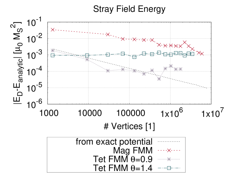
Figure 7: This plot shows the stray-field energy error for the algorithms compared in fig. 6.

Figure 7 shows the difference of the stray-field energy to the analytically computed energy ($E_{analytic}=1/6\mu_{0}M_{S}^{2}$). The E error is not constant because the multipole levels increase with the problem size and the real $theta$ depends on the varying octree dissection of the mesh. As an estimate the constant error for more than 1 million vertices results to $\Delta E\approx 10^{-3}\mu_{0}M_{S}^{2}$ for maximum multipole order $O=4$ and a $\Delta E\approx 3\times 10^{-4}\mu_{0}M_{S}^{2}$ for $O=6$ respectively. A smaller error can be achieved by changing the MAC $\theta$ and multipole order at a performance cost.

The error of the Mag FMM code is caused by the non-continuous nature of the sources; it is much lower for atomistic scales when sources are set into the crystal lattice points and the problem becomes non-continuous. The theoretical optimum was computed using the analytically computed potential at each vertex. If the $H$-field is computed directly — which is the case for some other methods — lower errors can be achieved.

To show the scaling properties of the code strong scaling on a single node is shown in fig. 8. It is easy to see that the code scales nearly optimally up to the 16 available cores. This indicates that it is compute- instead of memory-bound and that it would profit more by the next hardware generations than most other methods currently in use.

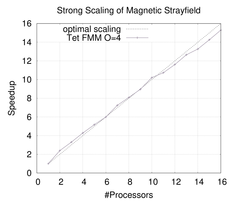
Figure 8: This plot shows how the TetFMM code scales on a single node up to 16 cores. Simulations were done with a $\theta=0.3$ and a multipole order $O=4$ on 357 911 vertices.

5 Conclusion

Nowadays, many core algorithms’ bottleneck is transfer speed and the trend seems to continue in that direction. The scaling properties of FMM are linear up to many processors and even GPUs[23]. The numeric results show that FMM computation today is comparable in speed to fast FEM implementations when the potential is required for calculation. In short the presented FMM is a good fit for micromagnetic calculations now and in the future.

6 Acknowledgment

The authors acknowledge the Vienna Science and Technology Fund (WWTF) under Grant No. MA14-044, the Austrian Science Fund (FWF): F41 SFB ViCoM and the the CD-Laboratory AMSEN (financed by the Austrian Federal Ministry of Economy, Family and Youth, the National Foundation for Research, Technology and Development) for financial support. The computational results presented have been achieved using the Vienna Scientific Cluster (VSC).

Appendix A Explicit Integrals for the Direct Integration

$${\int_{T}\frac{\mathbf{1}}{{\left(x_{t}^{2}+y_{t}^{2}+h^{2}\right)}^{\frac{3}{2}}}\mathrm{d}x_{t}\mathrm{d}y_{t}}=\int_{y-}^{y+}\left(\frac{x}{(h^{2}+y^{2})\sqrt{h^{2}+x^{2}+y^{2}}}\right)\Bigg{|}_{x=x-}^{x+}\mathrm{d}y_{t}$$ (7)

$${\int_{T}\frac{\mathbf{y_{t}^{2}}}{{\left(x_{t}^{2}+y_{t}^{2}+h^{2}\right)}^{\frac{3}{2}}}\mathrm{d}x_{t}\mathrm{d}y_{t}}\\ =\int_{y-}^{y+}\left(\frac{xy^{2}}{\left(h^{2}+y^{2}\right)\sqrt{h^{2}+x^{2}+y^{2}}}\right)\Bigg{|}_{x=x-}^{x+}\mathrm{d}y_{t}$$ (8)

$${\int_{T}\frac{\mathbf{x_{t}}}{{\left(x_{t}^{2}+y_{t}^{2}+h^{2}\right)}^{\frac{3}{2}}}\mathrm{d}x_{t}\mathrm{d}y_{t}}=-\int_{y-}^{y+}\left(\frac{1}{\sqrt{h^{2}+x^{2}+y^{2}}}\right)\Bigg{|}_{x=x-}^{x+}\mathrm{d}y_{t}$$ (9)

$$=\frac{1}{\sqrt{h^{2}+\frac{{(x_{1}(y_{2}-y)+x_{2}(y-y_{1}))}^{2}}{{(y_{1}-y_{2})}^{2}}+y^{2}}}-\frac{1}{\sqrt{h^{2}+\frac{{(x_{1}(y_{2}-y)+x_{3}(y-y_{1}))}^{2}}{{(y_{1}-y_{2})}^{2}}+y^{2}}}$$

$${\int_{T}\frac{\mathbf{x_{t}y_{t}}}{{\left(x_{t}^{2}+y_{t}^{2}+h^{2}\right)}^{\frac{3}{2}}}\mathrm{d}x_{t}\mathrm{d}y_{t}}=-\int_{y-}^{y+}\left(\frac{y}{\sqrt{h^{2}+x^{2}+y^{2}}}\right)\Bigg{|}_{x=x-}^{x+}\mathrm{d}y_{t}$$ (10)

$$=f_{xy}(b1,k1,y)+g_{xy}(b1,k1,y)-f_{xy}(b2,k2,y)+g_{xy}(b2,k2,y)$$

with

$$f_{xy}(b,k,y)=\frac{\sqrt{b^{2}+h^{2}+2bky+y^{2}(1+k^{2})}}{1+k^{2}}$$

$$g_{xy}(b,k,y)=\frac{bk\ln(bk+y+k^{2}y+\sqrt{1+k^{2}}\sqrt{b^{2}+h^{2}+2bky+(1+k^{2})y^{2}})}{{(1+k^{2})}^{\frac{3}{2}}}$$

$$b1=x_{2}-y_{2}k_{1};\;k1=\frac{x_{1}-x_{2}}{y_{1}-y_{2}}$$

$$b1=x_{3}-y_{2}k_{3};\;k2=\frac{x_{1}-x_{3}}{y_{1}-y_{2}}$$

$${\int_{T}\frac{\mathbf{y_{t}}}{{\left(x_{t}^{2}+y_{t}^{2}+h^{2}\right)}^{\frac{3}{2}}}\mathrm{d}x_{t}\mathrm{d}y_{t}}$$ (11)

$$=\int_{x_{y-1}}^{x_{y+1}}{\left(\frac{1}{\sqrt{h^{2}+x^{2}+y^{2}}}\right)}\Bigg{|}_{y=y_{y-}}^{y=y_{y+}}\mathrm{d}x_{t}$$

$$+\int_{x_{y-2}}^{x_{y+2}}{\left(\frac{1}{\sqrt{h^{2}+x^{2}+y^{2}}}\right)}\Bigg{|}_{y=y_{y-}}^{y=y_{y+}}\mathrm{d}x_{t}$$

$$=-f_{2}(b1y,k1y,y_{1})-f_{2}(b2y,k2y,y_{2})+2\ln\left(x+\sqrt{h^{2}+x^{2}+y_{2}^{2}}\right)$$

$$f_{2}=\frac{\ln(bk+x+k^{2}x+\sqrt{1+k^{2}}\sqrt{b^{2}+h^{2}+2bkx+x^{2}+k^{2}x^{2}})}{\sqrt{1+x^{2}}}$$

$$b1y=y_{2}-x_{2}k1y;\;k1y=\frac{y_{1}-y_{2}}{x_{1}-x_{2}}$$

$$b2y=y_{1}-x_{1}k2y;\;k1y=\frac{y_{1}-y_{2}}{x_{1}-x_{3}}$$

References

- Abert et al. [2012] Claas Abert, Gunnar Selke, Benjamin Krüger, and André Drews. A fast finite-difference method for micromagnetics using the magnetic scalar potential. Magnetics, IEEE Transactions on, 48(3):1105–1109, 2012.
- Abert et al. [2013] Claas Abert, Lukas Exl, Gunnar Selke, André Drews, and Thomas Schrefl. Numerical methods for the stray-field calculation: A comparison of recently developed algorithms. Journal of Magnetism and Magnetic Materials, 326:176–185, January 2013. ISSN 0304-8853. doi: 10.1016/j.jmmm.2012.08.041.
- Beatson and Greengard [1997] Rick Beatson and Leslie Greengard. A short course on fast multipole methods. Wavelets, multilevel methods and elliptic PDEs, 1:1–37, 1997.
- Blue and Scheinfein [Nov./1991] J.L. Blue and M.R. Scheinfein. Using multipoles decreases computation time for magnetostatic self-energy. IEEE Transactions on Magnetics, 27(6):4778–4780, Nov./1991. ISSN 00189464. doi: 10.1109/20.278944.
- Brunotte et al. [1992] Xavier Brunotte, Gérard Meunier, and Jean-François Imhoff. Finite element modeling of unbounded problems using transformations: a rigorous, powerful and easy solution. IEEE Transactions on Magnetics, 28(2):1663–1666, 1992.
- Buchau et al. [2003] André Buchau, Wolfgang M. Rucker, Oliver Rain, V. Rischmuller, Stefan Kurz, and Sergej Rjasanow. Comparison between different approaches for fast and efficient 3-D BEM computations. IEEE transactions on magnetics, 39(3):1107–1110, 2003.
- Chang et al. [2011] R. Chang, S. Li, M. V. Lubarda, B. Livshitz, and V. Lomakin. Fastmag: Fast micromagnetic solver for large-scale simulations. CMRR Report, 34, 2011.
- Cheng et al. [1999] H. Cheng, L. Greengard, and V. Rokhlin. A Fast Adaptive Multipole Algorithm in Three Dimensions. Journal of Computational Physics, 155(2):468–498, November 1999. ISSN 0021-9991. doi: 10.1006/jcph.1999.6355.
- Chernyshenko and Fangohr [2016] Dmitri Chernyshenko and Hans Fangohr. Computation of the magnetostatic interaction between linearly magnetized polyhedrons. arXiv:1601.04185 [physics], January 2016.
- Exl and Schrefl [2014] L. Exl and T. Schrefl. Non-uniform FFT for the finite element computation of the micromagnetic scalar potential. Journal of Computational Physics, 270:490–505, August 2014. ISSN 0021-9991. doi: 10.1016/j.jcp.2014.04.013.
- Exl et al. [2012] L. Exl, W. Auzinger, S. Bance, M. Gusenbauer, F. Reichel, and T. Schrefl. Fast stray field computation on tensor grids. Journal of Computational Physics, 231(7):2840–2850, April 2012. ISSN 00219991. doi: 10.1016/j.jcp.2011.12.030.
- Fredkin and Koehler [1990] D. R. Fredkin and T. R. Koehler. Hybrid method for computing demagnetizing fields. Magnetics, IEEE Transactions on, 26(2):415–417, 1990.
- Graglia [1987] R.D. Graglia. Static and dynamic potential integrals for linearly varying source distributions in two- and three-dimensional problems. IEEE Transactions on Antennas and Propagation, 35(6):662–669, June 1987. ISSN 0018-926X. doi: 10.1109/TAP.1987.1144160.
- Greengard and Rokhlin [1987] Leslie Greengard and Vladimir Rokhlin. A fast algorithm for particle simulations. Journal of computational physics, 73(2):325–348, 1987.
- Knittel et al. [2009] A. Knittel, M. Franchin, G. Bordignon, T. Fischbacher, Simon Bending, and H. Fangohr. Compression of boundary element matrix in micromagnetic simulations. Journal of Applied Physics, 105(7):07D542, 2009.
- Livshitz et al. [2009] Boris Livshitz, Amir Boag, H. Neal Bertram, and Vitaliy Lomakin. Nonuniform grid algorithm for fast calculation of magnetostatic interactions in micromagnetics. Journal of Applied Physics, 105(7):07D541, 2009.
- Long et al. [2006] H. H. Long, E. T. Ong, Z. J. Liu, and E. P. Li. Fast Fourier transform on multipoles for rapid calculation of magnetostatic fields. Magnetics, IEEE Transactions on, 42(2):295–300, 2006.
- Popović and Praetorius [2004] N. Popović and D. Praetorius. Applications of -Matrix Techniques in Micromagnetics. Computing, 74(3):177–204, December 2004. ISSN 0010-485X, 1436-5057. doi: 10.1007/s00607-004-0098-7.
- Raykar [2005] Vikas Chandrakant Raykar. A short primer on the fast multipole method. Available online on the author’s website, 1, 2005.
- Tsukerman et al. [1998] Igor Tsukerman, Alexander Plaks, and H. Neal Bertram. Multigrid methods for computation of magnetostatic fields in magnetic recording problems. Journal of applied physics, 83(11):6344–6346, 1998.
- Visscher and Apalkov [2010] P. B. Visscher and D. M. Apalkov. Simple recursive implementation of fast multipole method. Journal of Magnetism and Magnetic Materials, 322(2):275–281, January 2010. ISSN 0304-8853. doi: 10.1016/j.jmmm.2009.09.033.
- Yokota et al. [2013] R. Yokota, D. Koyama, C.-H. Lai, and N. Yamamoto. An FMM based on dual tree traversal for many-core architectures. Journal of Algorithms & Computational Technology, 7(3):301–324, 2013.
- Yokota and Barba [2012] Rio Yokota and Lorena A. Barba. A tuned and scalable fast multipole method as a preeminent algorithm for exascale systems. International Journal of High Performance Computing Applications, 26(4):337–346, 2012.
- Zhang et al. [2009] Linbo Zhang, Tao Cui, Hui Liu, and others. A set of symmetric quadrature rules on triangles and tetrahedra. J. Comput. Math, 27(1):89–96, 2009.
- Zhang and Haas [2009] Wen Zhang and Stephan Haas. Adaptation and performance of the Cartesian coordinates fast multipole method for nanomagnetic simulations. Journal of Magnetism and Magnetic Materials, 321(22):3687–3692, November 2009. ISSN 03048853. doi: 10.1016/j.jmmm.2009.07.016.