Skyrmions confined as beads on a vortex ring

Abstract

A very simple, quadratic potential is used to construct vortex strings in a generalized Skyrme model and an additional quadratic potential is used to embed sine-Gordon-type halfkinks onto the string worldline, yielding half-Skyrmions on a string. The strings are furthermore compactified onto a circle and the halfkinks are forced to appear in pairs; in particular $2B$ halfkinks (half-Skyrmions) will appear as beads on a ring with $B$ being the number of times the host vortex is twisted and also the baryon number (Skyrmion number) from the bulk point of view. Finally, we construct an effective field theory on the torus, describing the kinks living on the vortex rings.

I Introduction

Among various topological solitons, Skyrmions are the ones having the longest history Skyrme:1962vh ; Skyrme:1961vq . Nevertheless they are still under active consideration, partly because they have been proposed to be identified with baryons of (large-$N_{c}$) QCD and provide a first-principles angle to nuclear physics; for some recent results see e.g. Gudnason:2016mms ; Haberichter:2015qca ; Karliner:2015qoa ; Adam:2015lra ; Foster:2015cpa ; Adam:2015rna ; Lau:2014baa .

In a series of papers, we have studied a number of different incarnations of Skyrmions Nitta:2012wi ; Nitta:2012rq ; Gudnason:2014hsa ; the simplest form is just the Skyrmion Skyrme:1962vh ; Skyrme:1961vq , whereas the topological charge of the Skyrmion – the baryon number – can be absorbed into a host soliton, yielding a daughter soliton living in the world volume of its host or mother soliton. The simplest incarnation is taking a domain wall and embedding either a baby-Skyrmion or a lump in its world volume Gudnason:2014nba ; this gives a Skyrmion from the bulk point of view, but of course with infinite energy due to the infinite (2+1)-dimensional world volume of the domain wall.

Another class of incarnations of Skyrmions is to construct a vortex string with a U(1) modulus and subsequently twist said modulus which will form kinks on the worldline of the string; each kink will correspond to either a half or a full baryon charge, depending on whether the kink winds $\pi$ or $2\pi$ which in turn is determined by the type of potential in the model. In Ref. Gudnason:2014jga we explicitly constructed a vortex string in compactified form; that is, compactified onto a circle. The potential used in Ref. Gudnason:2014jga was inspired by a limit of a potential used in Bose-Einstein condensates (BEC) Ruostekoski:2001fc ; Battye:2001ec (see also Kawakami:2012zw ; Nitta:2012hy ) and it breaks a U(2) subgroup of the O(4) symmetry of the Skyrme model to U(1)$\times$U(1); one of them is used for constructing the vortex and the other will be the mentioned U(1) modulus living on the string worldline. In Ref. Gudnason:2014hsa we constructed straight vortex strings using the same BEC potential and embedded kinks and halfkinks on their worldlines. The last possibility in this direction is to compactify the strings and embed kinks on them; in this case the number of kinks is forced to be integer as the baryon number is quantized for finite energy configurations; this implies that when the vortex ring possesses halfkinks, it must have an even number of halfkinks. This case of a vortex ring with embedded kinks on its worldline has not been explicitly constructed before; this will be a new result in the present paper. A lower dimensional analog, however, has been studied in the baby-Skyrme model in 2+1 dimensions Kobayashi:2013ju by compactifying a domain wall worldline, with baby-Skyrmions on it Nitta:2012xq , to a circle.

The last incarnation of Skyrmions is a half-Skyrmion inside a monopole Gudnason:2015nxa . The unit-charged Skyrmion is split into a set of monopole and anti-monopole both of which carry a half baryon number. If a half-Skyrmion is separated from its other half, then it will have a divergent total energy because it is a global monopole. This also has a lower dimensional analogue in the baby-Skyrme model Kobayashi:2013aja , in which case half a baby-Skyrmion lives inside a global vortex.

Besides the four-dimensional incarnations of Skyrmions, in five dimensions it is possible to create a string with Skyrme charge that ends on a domain wall Gudnason:2014uha ; interestingly, this is possible in the O(4) model, which is just the standard Skyrme model (but generalized to 4+1 dimensions).

In this paper, we show that there exists a simpler potential than the BEC-type potential used in Refs. Gudnason:2014jga ; Gudnason:2014hsa admitting a vortex string and vortex rings. Using a notation with two complex fields $\phi_{1,2}\in\mathbb{C}$, the BEC-type potential is of the form $|\phi_{1}|^{2}(1-|\phi_{1}|^{2})$, whereas the simplest possibility for forming a vortex string is the potential we study in this paper, i.e. of the form $(1-|\phi_{1}|^{2})$. An interesting side mark about this potential is that it is induced at the classical level by introducing an isospin-breaking chemical potential of the form $\partial_{0}U\to\partial_{0}U-i[\mu\sigma^{3},U]$. However, this chemical potential – at the classical level – also induces other terms; in particular, the Skyrme term induces a noncanonical kinetic term which effectively can drive the coefficient of the kinetic term negative for large enough $\mu$. Although such chemical potential at the classical level, has been discussed in the literature Loewe:2004ic ; Loewe:2005kq ; Loewe:2006hv ; Ponciano:2007jm , Ref. Cohen:2008tf pointed out that due to a subtlety in the large-$N_{c}$ counting of $\mu$, one should not include the effects of the chemical potential at the classical level if one wishes to study the proton or neutron, because the large-$N_{c}$ nature of the model will pick out the largest spin state of the nucleon; hence not the proton or neutron. Therefore, if one does not include the effect of the chemical potential at the classical level, there is no presence of the potential that we use to construct vortex strings. We also do not consider the other terms that would be induced from said chemical potential. We simply take the potential and prove that it can be used to construct strings in the Skyrme model.

In this paper, as in Refs. Gudnason:2014hsa ; Gudnason:2014jga ; Gudnason:2013qba ; Gudnason:2014gla ; Gudnason:2015nxa , we compare the Skyrme term to the sixth-order derivative term, which is composed by squaring the baryon current; this term is inspired by the BPS-Skyrme model Adam:2010fg ; Adam:2010ds ; Adam:2015ele . The BPS-Skyrme model was motivated by the long-standing problem of the large binding energies in the standard Skyrme model; in the BPS-Skyrme model, which is a particular submodel of the Skyrme model, the BPS bound can be saturated – unlike Manton:1986pz the one in the standard Skyrme model Faddeev:1976pg – and so classically the binding energies vanish.

Finally, in Ref. Gudnason:2014gla we constructed a framework of effective field theories for solitons living on host solitons of generic shapes. In Ref. Gudnason:2014gla we applied it to straight vortices with the BEC potential. In this paper, we will use the same framework for the vortices in the new potential and use it to construct kinks directly in the effective field theory approach. Finally, as a new result, we derive the effective field theory for sine-Gordon halfkinks living on vortex rings – that is, vortex strings compactified onto a circle – and use it to calculate the kinks and baryon charge density in the effective theory approach.

The paper is organized as follows. In Sec. II we introduce the model, set the notation and discuss the vacua and symmetries. In Sec. III we construct the straight, infinitely long, vortex string, which we in Sec. IV compactify onto a circle with one and two twists, yielding a $B=1$ and $B=2$ vortex ring, respectively. In Sec. V we then, finally, embed kinks onto both the straight vortex and the vortex ring and we also construct the relevant leading-order effective field theories for all cases. We conclude in Sec. VI with a discussion of our results. The appendix A provides evidence for the two-vortex to split up into two separate Skyrmions.

II Skyrme-like model

We consider a Skyrme-type model in 3+1 dimensions

$$\mathcal{L}=\frac{1}{4}{\rm Tr}(L_{\mu}L^{\mu})+c_{4}\mathcal{L}_{4}+c_{6}\mathcal{L}_{6}-V(U),$$ (1)

that includes the Skyrme term and a sixth-order term – made of the square of the baryon current – which we will call the BPS-Skyrme term Adam:2010fg ; Adam:2010ds ; Adam:2015ele ,

$$\mathcal{L}_{4} =\frac{1}{32}{\rm Tr}\left([L_{\mu},L_{\nu}]^{2}\right),$$ (2)

$$\mathcal{L}_{6} =\frac{1}{144}\left(\epsilon^{\mu\nu\rho\sigma}{\rm Tr}\left[L_{\nu}L_{\rho}L_{\sigma}\right]\right)^{2},$$ (3)

where we have defined the $\mathfrak{su}(2)$-valued left-invariant current $L_{\mu}\equiv U^{\dagger}\partial_{\mu}U$, $U$ is the 2-by-2 nonlinear sigma-model field obeying the constraint $U^{\dagger}U=\mathbf{1}_{2}$, the spacetime indices $\mu,\nu,\rho,\sigma=0,1,2,3$ run over all 3+1 dimensions, the Lagrangian coefficients $c_{4}\geq 0$ and $c_{6}\geq 0$ are both positive semi-definite and finally, we use the mostly-positive metric signature.

Since (one of) our objective(s) is to study vortices, it will prove convenient to switch notation from the matrix field $U$ to a complex vector field $\phi$ as

$$\phi\equiv\begin{pmatrix}\phi_{1}\\ \phi_{2}\end{pmatrix}.$$ (4)

The two fields are related as follows

$$U=\begin{pmatrix}\phi&-i\sigma^{2}\phi^{*}\end{pmatrix}=\begin{pmatrix}\phi_{1}&-\phi_{2}^{*}\\ \phi_{2}&\phi_{1}^{*}\end{pmatrix},$$ (5)

and the nonlinear sigma-model constraint translates to

$$\det U=|\phi_{1}|^{2}+|\phi_{2}|^{2}=1.$$ (6)

Rewriting the Lagrangian density (1) using the field $\phi$, we get

$$\mathcal{L}=-\frac{1}{2}\partial_{\mu}\phi^{\dagger}\partial^{\mu}\phi+c_{4}\mathcal{L}_{4}+c_{6}\mathcal{L}_{6}-V(\phi,\phi^{\dagger}),$$ (7)

where the Skyrme term and BPS-Skyrme term now read

$$\mathcal{L}_{4} =-\frac{1}{4}(\partial_{\mu}\phi^{\dagger}\partial^{\mu}\phi)^{2}+\frac{1}{16}(\partial_{\mu}\phi^{\dagger}\partial_{\nu}\phi+\partial_{\nu}\phi^{\dagger}\partial_{\mu}\phi)^{2},$$ (8)

$$\mathcal{L}_{6} =\frac{1}{4}\left(\epsilon^{\mu\nu\rho\sigma}\phi^{\dagger}\partial_{\nu}\phi\partial_{\rho}\phi^{\dagger}\partial_{\sigma}\phi\right)^{2}.$$ (9)

The Lagrangian density (1) enjoys manifest $\mathrm{SU}(2)\times\mathrm{SU}(2)$ symmetry when the potential is switched off; this symmetry is however spontaneously broken to its diagonal subgroup, $\mathrm{SU}(2)\times\mathrm{SU}(2)\to\mathrm{SU}(2)$ by the presence of any finite-energy configuration. Turning on a mass term for the pions, e.g. $V\sim{\rm Tr}[\mathbf{1}_{2}-U]$, results in the same symmetry breaking, however explicitly. This symmetry breaking is important because it is the basis of the existence of the Skyrmion or simply baryon charge. The Skyrmions are characterized by the degree of the map from space with infinity identified as a point ($\mathbb{R}^{3}\cup\{\infty\}\simeq S^{3}$) to SU(2),

$$\pi_{3}({\rm SU}(2))\simeq\pi_{3}(S^{3})=\mathbb{Z}\ni B.$$ (10)

The integer $B$ is the degree, the topological charge or simply the baryon number, and can be calculated from a configuration as

$$B =-\frac{1}{24\pi^{2}}\int d^{3}x\;\epsilon^{ijk}\,{\rm Tr}\left(L_{i}L_{j}L_{k}\right)$$

$$=-\frac{1}{4\pi^{2}}\int d^{3}x\;\epsilon^{ijk}\phi^{\dagger}\partial_{i}\phi\partial_{j}\phi^{\dagger}\partial_{k}\phi.$$ (11)

In order to construct a vortex in our model at hand, we need a special potential that breaks the symmetry explicitly and further than to simply SU(2). One such potential – which was inspired by Bose-Einstein condensates Ruostekoski:2001fc ; Battye:2001ec – was considered in Ref. Gudnason:2014hsa . That potential is fourth order in $\phi$ and of the form $|\phi_{1}\phi_{2}|^{2}=|\phi_{1}|^{2}(1-|\phi_{1}|^{2})$. This potential breaks the symmetry of the model to U(1)$\times$U(1), explicitly. One of the U(1)s are then used to construct the vortex and the other manifests itself as a U(1) modulus living on the vortex worldsheet.

In this paper, we show that there is an even simpler potential than that considered in Ref. Gudnason:2014gla ; Gudnason:2014hsa , which allows for vortices in the model and it reads

$$V^{\rm vortex}=\frac{1}{2}m^{2}\left(1-\frac{1}{2}\phi^{\dagger}(\mathbf{1}_{2}+\tau^{3})\phi\right)=\frac{1}{2}m^{2}\left(1-|\phi_{1}|^{2}\right).$$ (12)

This is one of the purposes of this paper, namely to construct the vortex strings in the simplest potential in Skyrme-type models.

Although not manifest in the formulation of the Lagrangian (7) in terms of $\phi$, it contains a symmetry group Gudnason:2014hsa – which is a subgroup of O(4) – in the absence of the potential term

$$\tilde{G}\simeq\mathrm{U}(2),$$ (13)

which can be seen as formed by

$$\mathrm{U}(2)\simeq\mathrm{SU}(2)_{\rm L}\times\mathrm{U}(1)_{\rm R},$$ (14)

where the latter U(1) group is generated by $\tau^{3}$ in SU(2)_R. The potential that allows for vortices will break

$$\tilde{G}\to G=\mathrm{U}(1)_{0}\times\mathrm{U}(1)_{3},$$ (15)

explicitly; U(1)₀ is the tracepart of U(2) and U(1)₃ is the U(1) subgroup of SU(2). Explicitly, each group acts on $\phi$ as

$$\mathrm{U}(1)_{0}: \qquad\phi\to e^{i\alpha}\phi,$$ (16)

$$\mathrm{U}(1)_{3}: \qquad\phi\to e^{i\beta\tau^{3}}\phi.$$ (17)

Unlike the potential that was considered in Ref. Gudnason:2014hsa which possessed two distinct vacua with in turn each of their kind of vortices, the potential (12) only has the vacuum

$$\langle\phi\rangle^{\rm T}=(e^{i\alpha},0),$$ (18)

and the unbroken symmetry group $H$ is

$$H=\mathrm{U}(1)_{0-3}: \qquad\phi\to e^{i\alpha(\mathbf{1}_{2}-\tau^{3})}\phi.$$ (19)

We can therefore write the moduli space as

$$\mathcal{M}\simeq G/H=\frac{\mathrm{U}(1)_{0}\times\mathrm{U}(1)_{3}}{\mathrm{U}(1)_{0-3}}\simeq\mathrm{U}(1)_{0+3},$$ (20)

which in turn gives rise to the nontrivial homotopy group

$$\pi_{1}(\mathcal{M})=\mathbb{Z}\ni n,$$ (21)

which admits vortices and we will denote the vortex winding number by $n$.

Although, as mentioned above, the system at hand generally contains also nonzero baryon charge, the straight vortex in this model does not a priori contain such. Inside the core of the vortex $|\phi_{1}|\simeq 0$ and so the vortex carries a U(1) modulus, $|\phi_{2}|\simeq 1$. In order for the configuration to acquire baryon charge, we need to twist the modulus; that is, the modulus needs to wind along the string. A $2\pi$ winding of the U(1) modulus corresponds topologically to a single sine-Gordon kink on the vortex worldsheet.

Let us explicitly construct a potential that gives rise to (sine-Gordon) kinks

$$V^{\rm kink}=-\frac{1}{2}m_{2}^{2}\left(\Re\phi_{2}\right)^{2}.$$ (22)

Now with the addition of this kink potential, we should discuss the vacuum manifold again in order to assess the topological charges present in the theory.

The total potential is given by

$$V=V^{\rm vortex}+V^{\rm kink}=\frac{1}{2}m^{2}\cos^{2}v-m_{2}^{2}\cos^{2}v\cos^{2}\beta,$$ (23)

where we have parametrized the field configuration as

$$\langle\phi\rangle^{\rm T}=(e^{i\alpha}\sin v,e^{i\beta}\cos v),$$ (24)

with $\alpha,\beta,v\in[0,2\pi)$, and thus for $m>m_{2}$, the vacuum solution is

$$v=\frac{\pi}{2}+q\pi,\qquad$$ (25)

where $q\in\mathbb{Z}$ is an integer that we without loss of generality can set to zero: $q=0$, and $\beta$ is undetermined. For $m<m_{2}$ there exists another vacuum which possesses no vortices and the vacuum solution is $v=q\pi$ and $\beta=q^{\prime}\pi$ with $q^{\prime}\in\mathbb{Z}$. For both solutions $V^{\rm vortex}+V_{2}^{\rm kink}=0$ in the vacua. Since we are interested in vortices, which exist only in the first case we will choose $m>m_{2}$ and hence the first vacuum solution. It is important here to note that the vacuum manifold, with the addition of the quadratic kink potential, is unchanged with respect to the one for only the vortex potential (20). Thus

$$\mathcal{M}_{V^{\rm vortex}+V^{\rm kink}}=\mathcal{M}_{V^{\rm vortex}}=U(1)_{0+3}.$$ (26)

We can think of the vortex solution in the following way. If we identify $\alpha=\phi$ to be the winding phase and $\sin v$ to be the radial profile function of the vortex, then $\beta$ is a U(1) modulus field living on the vortex string when the kink potential is turned off. When we turn on the kink potential $m_{2}>0$, then although $\beta$ can take any value in the vacuum, $\beta=q^{\prime}\pi$ induces the smallest vortex mass (and thus smallest vortex tension); the vacua of the modulus on the string worldsheet are $\beta=q^{\prime}\pi$, again with $q^{\prime}\in\mathbb{Z}$.

We can now evaluate the topological kink number on the vortex core. The vortex core is defined by $\phi_{1}=0$ and so due to the nonlinear sigma model constraint (6), we have $|\phi_{2}|=1$. In the parametrization (24) this corresponds to $v=q\pi$ and the vacua for $\beta=q^{\prime}\pi$ on the string worldsheet as mentioned just above. The topological kink number is thus

$$\pi_{0}(\mathcal{M}^{\rm vortex})=\pi_{0}(\mathbb{Z})=\mathbb{Z}\ni k,$$ (27)

where $k$ is the number of sine-Gordon halfkinks. We define these kinks to be halfkinks because they only wind $\pi$ in the U(1) modulus, as compared to $2\pi$, for which we would call the kinks full kinks or simply kinks.

The baryon number in the bulk of the total system can be calculated as

$$B=\frac{nk}{2},$$ (28)

where $n$ is the vortex number and $k$ is the sine-Gordon halfkink number.

III The straight vortex

We are now ready to construct the vortex in the model introduced in the last section. With no potential, a string-like configuration is of course unstable to decay Nitta:2007zv , but the potential (12) considered here admits a stable vortex string. We begin with the case where the vacuum is at $|\phi_{1}|=1$ and so $v=\pi/2$. This for the kinkless case: $m_{2}=0$. Now we can choose an appropriate Ansatz for the vortex as

$$\phi_{1}=\sin f(r)e^{i\phi},\qquad\phi_{2}=\cos f(r)e^{i\chi},$$ (29)

where $f(r)$ is the profile of the vortex and $(r,\phi)$ are polar coordinates in the $xy$-plane: $x=r\cos\phi$ and $y=r\sin\phi$. The constant $\chi$ is the U(1) modulus residing on the vortex string and in this section we take it to be its vacuum value which is $\chi=q^{\prime}\pi$ and so without loss of generality we can set $\chi=0$. Inserting the above Ansatz into the Lagrangian density (7), we get

$$-\mathcal{L}=\frac{1}{2}f_{r}^{2}+\frac{1}{2r^{2}}\sin^{2}f+\frac{c_{4}}{2r^{2}}\sin^{2}(f)f_{r}^{2}+\frac{1}{2}m^{2}\cos^{2}(f),$$ (30)

which by variation with respect to the vortex profile function $f$, leads to the equation of motion

$$f_{rr}+\frac{1}{r}f_{r}-\frac{1}{2r^{2}}\sin 2f+\frac{c_{4}}{r^{2}}\sin^{2}f\left(f_{rr}-\frac{1}{r}f_{r}\right)+\frac{c_{4}}{2r^{2}}\sin(2f)f_{r}^{2}+\frac{1}{2}m^{2}\sin 2f=0,$$ (31)

where $f_{r}\equiv\partial_{r}f$, etc. In order to construct a vortex solution, we need to impose the following boundary conditions on the vortex profile function $f$,

$$f(0)=0,\qquad f(\infty)=\frac{\pi}{2}.$$ (32)

First notice that the vortex Lagrangian density does not contain any term stemming from the sixth-order BPS-Skyrme term present in Eq. (7). This is clear because first when the vortex string has a nontrivial dependence along the string (the $z$-direction in our frame), then the baryon charge operator (which is the square root of the BPS-Skyrme term) can acquire nonvanishing values.

Around $r=0$ we can expand $f$ in a power series in $r$ and expanding the equation of motion (31) up to third order, determines $f$ up to fifth order

$$f=f_{1}r-\frac{24f_{1}+f_{1}^{3}-2f_{1}^{5}}{12+48f_{1}^{2}}\,r^{3}+\mathcal{O}(r^{5}),$$ (33)

in terms of $f_{1}$, which is called the shooting parameter and encodes nonperturbative information about the vortex. Expanding instead the vortex profile function around spatial infinity leads to

$$f\simeq{\mathop{\rm gd}}(mr),$$ (34)

where ${\mathop{\rm gd}}$ is the Gudermannian function defined by ${\mathop{\rm gd}}(z)\equiv 2\mathop{\mathrm{arctan}}\nolimits(e^{z})-\pi/2$.

A comment in store is about the energy. The energy density for static configurations is simply given by $-\mathcal{L}$, where the Lagrangian density is that of Eq. (30). The total energy, however, diverges, in more than one (spatial) direction. Considering first the plane transverse to the vortex (for concreteness we can choose this plane to be the $xy$-plane), the vortex tension diverges logarithmically because the vortex is a global vortex . Next, if the vortex is not compactified on a circle, i.e. if it is an infinitely long straight string, then the total energy diverges like $L\log L$, where $L$ is a cutoff in length scale.

Let us now consider the tension in more detail. As we already mentioned, the tension (energy per unit length) diverges logarithmically. Let us consider the contributions from the different terms to the asymptotic tension, by plugging the asymptotic form of the profile function (34) into the energy ($-\mathcal{L}$ in Eq. (30)) and integrate over the $xy$-plane (the plane transverse to the vortex). The kinetic term has two contributions to the energy

$$\lim_{R\to\infty}\left[\int dr\;rf_{r}^{2}\sim\int dr\;\frac{2me^{mr}}{1+e^{2mr}}=2r\mathop{\mathrm{arctan}}\nolimits e^{mr}-\frac{i}{m}\mathop{\mathrm{Li}}\nolimits_{2}\left(-ie^{mr}\right)+\frac{i}{m}\mathop{\mathrm{Li}}\nolimits_{2}\left(ie^{mr}\right)\right]^{r=R}=0,$$

$$\int^{R}dr\;\frac{1}{r}\sin^{2}f\sim\int^{R}dr\;\frac{\tanh^{2}mr}{r}\sim\log R,$$ (35)

but only the latter diverges (logarithmically). The contribution from the Skyrme term, however, is finite

$$\lim_{R\to\infty}\left[\int dr\;\frac{1}{r}\sin^{2}(f)f_{r}^{2}\sim\int dr\;\frac{m}{r}\mathop{\mathrm{sech}}\nolimits mr\tanh mr\right]^{r=R}=0,$$

as is that of the potential

$$\lim_{R\to\infty}\left[\int dr\;rm^{2}\cos^{2}f\sim\int dr\;\frac{m^{2}re^{2mr}}{(1+e^{2mr})^{2}}=\frac{mR(1+\tanh mR)-\log[1+e^{2mR}]}{4}\right]^{r=R}=0.$$

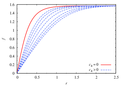
(a)

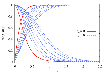
(b)

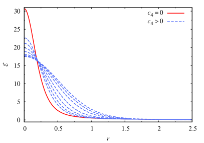
(c)

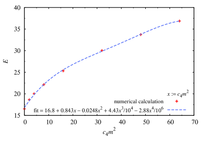
(d)

Figure 1: Vortex solutions for various values of $c_{4}=0,0.125,0.25,0.5,1,2,3,4$: (a) profile function $f$, (b) the condensate $|\phi_{1}|=\sin f$ and $|\phi_{2}|=\cos f$, (c) energy density and (d) total energy. For the figure we have fixed the length scales by setting $m=4$.

As the equation of motion (31) cannot be solved analytically, we turn to numerically methods; namely we use a fourth-order Runge-Kutta method to find numerical solutions for various values of $c_{4}$. The solutions, the corresponding condensate, energy densities and integrated energies are shown in Fig. 1.

The mass parameter $m$ can be scaled away and physically just corresponds to setting the length scale. The only free parameter in the system is then $c_{4}m^{2}$ which turns on the Skyrme term and results in a wider vortex string. The energy density of the wider vortex string is likewise wider but also has a lower density at the vortex core, see Fig. 1(c). The total energy, however, increases monotonically as function of $c_{4}m^{2}$, as expected, see Fig. 1(d).

IV Vortex rings as Skyrmions

In this section, we study the vortex ring in the simpler vortex potential (12) as compared to that considered in Refs. Gudnason:2014gla ; Gudnason:2014jga ; Gudnason:2014hsa . We will consider this potential in two variants of our model, which we shall call the 2+4 model and the 2+6 model

$$2+4\;{\rm model}:\quad c_{4}=1,\quad c_{6}=0,$$ (36)

$$2+6\;{\rm model}:\quad c_{4}=0,\quad c_{6}=1.$$ (37)

This choice of coefficients is made such that we can see the differences between the normal Skyrme term and the sextic term of the BPS-Skyrme model.

Since the potential (12) breaks spherical symmetry and the potential (22) furthermore breaks axial symmetry, we will perform the numerical calculations of the partial differential equations (equations of motion) on a cubic lattice using the finite difference method in conjunction with the relaxation method. We typically use $121^{3}$ lattices, but also smaller lattices like $81^{3}$ and $101^{3}$, where the denser grid is not necessary. We should warn the reader that the configurations shown in the figures are cropped to better show the features of the plots and thus the size of the grids used appears to be smaller than what was used for the calculations.

IV.1 Singly twisted vortex rings as Skyrmions

We start by performing numerical calculations of the standard hedgehog Skyrmion in the 2+4 model, gradually turning on the vortex potential (12). Our initial condition for the relaxation method is taken as the hedgehog Ansatz in the following form

$$\phi_{\rm initial}^{\rm T}=\left(\cos f-i\sin f\cos\theta,e^{i\phi}\sin f\sin\theta\right).$$ (38)

Figs. 3 and 3 show $xy$-slices at $z=0$ of the baryon charge densities and energy densities for the single Skyrmion in the 2+4 model for various values of the vortex potential mass parameter $m=0,1,\ldots,7$. As can be seen from the figures, all the Skyrmion configurations are nearly spherical and so we have shown only the $xy$-slices.

(a)

(b)

(c)

(d)

(e)

(f)

(g)

(h)

Figure 2: Single vortex ring in the 2+4 model. The figure is an $xy$-slice of the baryon charge density at $z=0$ for the vortex potential mass parameter $m=0,1,2,3,4,5,6,7$ from top-left to bottom-right panel.

(a)

(b)

(c)

(d)

(e)

(f)

(g)

(h)

Figure 3: Single vortex ring in the 2+4 model. The figure is an $xy$-slice of the energy density at $z=0$ for the vortex potential mass parameter $m=0,1,2,3,4,5,6,7$ from top-left to bottom-right panel.

In fact, the only effect of the vortex potential on the Skyrmion solutions other than shrinking them and increasing their energies, is that their spherical symmetry gets broken; that is, they become slightly squashed spheres. To measure the squashing of the Skyrmions as function of the vortex potential mass parameter $m$, we define

$$(x_{B}^{i})^{2}\equiv\frac{1}{B}\int d^{3}x\;(x^{i})^{2}\mathcal{B},$$ (39)

$i$ not summed over and

$$\mathcal{B}=-\frac{1}{4\pi^{2}}\epsilon^{ijk}\phi^{\dagger}\partial_{i}\phi\partial_{j}\phi^{\dagger}\partial_{k}\phi^{\dagger},$$ (40)

is the baryon charge density. Then the size in one spatial direction is taken as $x_{B}^{i}=\sqrt{(x_{B}^{i})^{2}}$. In Fig. 4 we show the ratio of the size in the $z$-direction to the $x$-direction (for these configurations $x_{B}=y_{B}$).

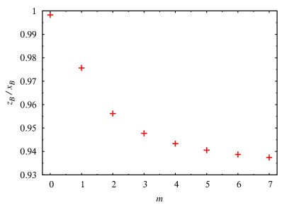
Figure 4: The ratio of the square root of the second moment of the baryon charge density in the $z$ and in the $x$ direction, $z_{B}/x_{B}$, for the single vortex ring in the 2+4 model as function of the vortex potential mass parameter $m$.

Next, we will turn to the 2+6 model, in which the vortex potential has a quite different effect on the Skyrmion. Figs. 6 and 6 show $xy$-slices at $z=0$ and $xz$-slices at $y=0$, respectively, of the baryon charge densities for the single Skyrmion in the 2+6 model for various values of the vortex potential mass parameter $m=0,1,\ldots,7$, while Figs. 8 and 8 show $xy$-slices at $z=0$ and $xz$-slices at $y=0$, respectively, of the energy densities.

(a)

(b)

(c)

(d)

(e)

(f)

(g)

(h)

Figure 5: Single vortex ring in the 2+6 model. The figure is an $xy$-slice of the baryon charge density at $z=0$ for the vortex potential mass parameter $m=0,1,2,3,4,5,6,7$ from top-left to bottom-right panel.

(a)

(b)

(c)

(d)

(e)

(f)

(g)

(h)

Figure 6: Single vortex ring in the 2+6 model. The figure is an $xz$-slice of the baryon charge density at $y=0$ for the vortex potential mass parameter $m=0,1,2,3,4,5,6,7$ from top-left to bottom-right panel.

We can see from Figs. 6 and 6 that the vortex potential turns (even) the single Skyrmion into a torus-like object. The dip in the baryon charge density at the center of the configuration starts to happen for a critical value of the vortex potential mass parameter $m_{\rm critical}$ between 2 and 3. In the last figure depicted in Fig. 6, the baryon charge density at the center of the Skyrmion is about 1/2 of the maximum value.

(a)

(b)

(c)

(d)

(e)

(f)

(g)

(h)

Figure 7: Single vortex ring in the 2+6 model. The figure is an $xy$-slice of the energy density at $z=0$ for the vortex potential mass parameter $m=0,1,2,3,4,5,6,7$ from top-left to bottom-right panel.

(a)

(b)

(c)

(d)

(e)

(f)

(g)

(h)

Figure 8: Single vortex ring in the 2+6 model. The figure is an $xz$-slice of the energy density at $y=0$ for the vortex potential mass parameter $m=0,1,2,3,4,5,6,7$ from top-left to bottom-right panel.

We observe also – analogously to what was seen in Ref. Gudnason:2014hsa – that the energy density is far more torus-like than the corresponding baryon charge density. The critical value of the vortex potential mass parameter $m$ for which a dip appears in the center of the Skyrmion is also lower than that for the baryon charge density and is between 1 and 2.

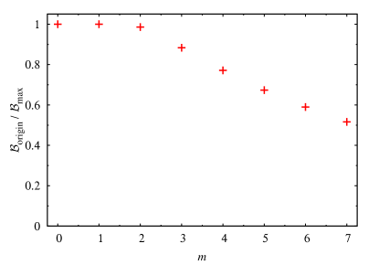
Figure 9: The ratio of the baryon charge density at the origin and the maximum baryon charge density, $\mathcal{B}_{\rm origin}/\mathcal{B}_{\rm max}$, for the single vortex ring in the 2+6 model as function of the vortex potential mass parameter $m$.

Finally, we show in Fig. 9 the ratio between the baryon charge density at the center (of mass) of the configuration to the maximum value, $\mathcal{B}(0)/\mathop{\rm max}(\mathcal{B}(x))$. It can be seen from the figure that the critical value for the dip to form is slightly smaller than, but about $m\lesssim 2$.

IV.2 Doubly twisted vortex rings as $B=2$ Skyrmions

In this subsection we consider the vortex rings of baryon charge $B=2$. As well known, the normal Skyrmion of charge $B=2$ already takes the shape of a torus; therefore we consider this case for completeness to study the effect of the vortex potential in the $B=2$ sector and it will serve as a basis for when we later in the paper want to add kinks to the $B=2$ vortex ring. Let us clarify that although $B=2$, the vortex has only vortex charge $n=1$ but it is twisted up twice, in our language.

As the initial condition for the $B=2$ Skyrmion, we use the following Ansatz

$$\phi_{\rm initial}^{\rm T}=\left(\cos f-i\sin f\cos\theta,e^{i2\phi}\sin f\sin\theta\right),$$ (41)

for an appropriate profile function $f$. This is of course just the standard axially symmetric generalization to $B=2$ of the hedgehog.

In Figs. 11 and 11 we show $xy$-slices at $z=0$ and $xz$-slices at $y=0$, respectively, of the baryon charge densities for the $B=2$ vortex ring in the 2+4 model for various values of $m=0,1,\ldots,7$, while in Figs. 13 and 13 we show the corresponding $xy$-slices at $z=0$ and $xz$-slices at $y=0$, respectively, of the energy densities. We see from the figures that the baryon charge densities and the energy densities are practically the same also in the $B=2$ case and so from now on we can focus on the baryon charge densities in the 2+4 model. We also note that turning on the vortex potential in the $B=2$ sector has a quite small effect on the 2+4 model; it merely shrinks the vortex ring and as a good approximation looks simply like a scale transformation on the $B=2$ Skyrmion without the vortex potential.

(a)

(b)

(c)

(d)

(e)

(f)

(g)

(h)

Figure 10: A $B=2$ vortex ring in the 2+4 model. The figure is an $xy$-slice of the baryon charge density at $z=0$ for the vortex potential mass parameter $m=0,1,2,3,4,5,6,7$ from top-left to bottom-right panel.

(a)

(b)

(c)

(d)

(e)

(f)

(g)

(h)

Figure 11: A $B=2$ vortex ring in the 2+4 model. The figure is an $xz$-slice of the baryon charge density at $y=0$ for the vortex potential mass parameter $m=0,1,2,3,4,5,6,7$ from top-left to bottom-right panel.

(a)

(b)

(c)

(d)

(e)

(f)

(g)

(h)

Figure 12: A $B=2$ vortex ring in the 2+4 model. The figure is an $xy$-slice of the energy density at $z=0$ for the vortex potential mass parameter $m=0,1,2,3,4,5,6,7$ from top-left to bottom-right panel.

(a)

(b)

(c)

(d)

(e)

(f)

(g)

(h)

Figure 13: A $B=2$ vortex ring in the 2+4 model. The figure is an $xz$-slice of the energy density at $y=0$ for the vortex potential mass parameter $m=0,1,2,3,4,5,6,7$ from top-left to bottom-right panel.

Next we turn to the 2+6 model and Figs. 15 and 15 show $xy$-slices at $z=0$ and $xz$-slices at $y=0$, respectively, of the baryon charge densities for the $B=2$ vortex ring for various values of $m=0,1,\ldots,7$, while in Figs. 17 and 17 show the corresponding slices of the energy densities.

Let us first warn the reader that the surface plots shown in the figures are cropped with respect to the calculations (which are done on far larger grids than shown here); so one should not worry about boundary effects from the lattice being a finite one.

As in the case of the 2+4 model, increasing the mass of the vortex potential $m$ has the effect of shrinking the vortex ring, however, in the 2+6 the hole in the torus actually grows, which is a big difference between the 2+6 and 2+4 models. Let us also note that the baryon charge densities have a quite distinct difference from their respective energy densities. The holes in the baryon charge densities are convex, whereas the holes in the energy densities turn from convex to concave as $m$ is increased. This is also a difference between the 2+6 and the 2+4 model.

(a)

(b)

(c)

(d)

(e)

(f)

(g)

(h)

Figure 14: A $B=2$ vortex ring in the 2+6 model. The figure is an $xy$-slice of the baryon charge density at $z=0$ for the vortex potential mass parameter $m=0,1,2,3,4,5,6,7$ from top-left to bottom-right panel.

(a)

(b)

(c)

(d)

(e)

(f)

(g)

(h)

Figure 15: A $B=2$ vortex ring in the 2+6 model. The figure is an $xz$-slice of the baryon charge density at $y=0$ for the vortex potential mass parameter $m=0,1,2,3,4,5,6,7$ from top-left to bottom-right panel.

(a)

(b)

(c)

(d)

(e)

(f)

(g)

(h)

Figure 16: A $B=2$ vortex ring in the 2+6 model. The figure is an $xy$-slice of the energy density at $z=0$ for the vortex potential mass parameter $m=0,1,2,3,4,5,6,7$ from top-left to bottom-right panel.

(a)

(b)

(c)

(d)

(e)

(f)

(g)

(h)

Figure 17: A $B=2$ vortex ring in the 2+6 model. The figure is an $xz$-slice of the energy density at $y=0$ for the vortex potential mass parameter $m=0,1,2,3,4,5,6,7$ from top-left to bottom-right panel.

One last consideration for the $B=2$ sector is whether the doubly wound vortex ($k=2$), twisted once is stable or not. In Ref. Gudnason:2014jga this case was studied in the BEC type vortex potential (as opposed to the simpler vortex potential considered here) and the findings were negative; that is, the $k=2$ vortex twisted once would decay into two separate $k=1$ vortices. The initial condition for the $k=2$ vortex ring twisted once is given by Gudnason:2014jga

$$\phi_{\rm initial}^{\rm T}=\left(\sqrt{1-\sin^{2}f\sin^{2}\theta}\,e^{i2\mathop{\mathrm{arctan}}\nolimits(\tan f\cos\theta)},\sin f\sin\theta\right).$$ (42)

All our numerical attempts at finding a $k=2$ vortex ring twisted once were unstable, so we conclude that the simpler vortex potential share the same instability as that of BEC type, see App. A.

V Confined Skyrmions

In this section we will consider the full potential (23); i.e. the vortex potential plus the kink potential. In particular, this potential allows for two kinks to be absorbed and confined on the vortex world sheet and in turn yielding a full unit of baryon charge from the bulk point of view.

In this section, we will begin with the straight vortex and then turn to embedding halfkinks on the vortex worldsheet. Then we curl up the vortex strings and the result will be an even number of kinks on the vortex ring; more precisely $2B$ kinks on a single vortex ring (with $B$ twists).

V.1 Straight vortex

It is straightforward to construct the straight vortex – without a kink on its worldsheet – but with the kink potential turned on. It suffices to see that with the Ansatz (29), the mass parameter $m$ in Sec. III should simply be replaced by

$$m_{\rm vortex}^{2}\equiv m^{2}-m_{2}^{2}>0.$$ (43)

All the discussion of Sec. III thus goes through.

The next step is to add the kink to the vortex world sheet, which we will turn to in the next subsection. First, however, we will compare the 3-dimensional solutions to 1-dimensional ones found in Sec. III.

V.1.1 Comparison of the PDE and ODE solutions for the vortex

Since the kink breaks translational symmetry along the vortex string, we need at least to consider a 2-dimensional partial differential equation (PDE). We choose however to work in Cartesian coordinates as in the last section, and calculate the vortex-kink system again on a cubic lattice using the relaxation method. Here we use a $121^{3}$ lattice with the smallest stepsize $\Delta x=\Delta y\simeq 0.025+0.017c_{4}$ and the largest stepsize is $\Delta z\simeq 1/(30m_{2})$.

Far from the kink, the vortex should be unaltered with respect to that found in Sec. III, except for the fact that the vortex mass $m$ is replaced with $m_{\rm vortex}$ in Eq. (43). We therefore – as a cross check on our calculations – compare the solutions found in Sec. III using the ordinary differential equation (ODE) and the Runge-Kutta method to the full 3D PDE solutions used in this section as bases for the kinks. The two vortex profiles are shown in Fig. 18, where the lines are ODE solutions and the points are PDE data. As we can see the lattice calculation gives exactly the same solution.

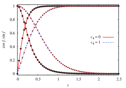
Figure 18: Comparison of vortex condensates between the ODE (points) and PDE (lines) calculations. Here the mass parameters are $m=4$ and $m_{2}=1$ giving the effective vortex mass $m_{\rm vortex}=\sqrt{15}\simeq 3.873$.

V.2 Halfkinks on a vortex as half-Skyrmions

In this section we twist the U(1) modulus of the vortex string, which gives rise to a kink on the vortex worldline and to a Skyrmion in the bulk volume (all space).

V.2.1 A single halfkink on a vortex as a half-Skyrmion

As mentioned already in the introduction, the fundamental kink in the (quadratic) kink potential is a halfkink, meaning that in terms of a U(1) modulus it winds only $\pi$ (as opposed to a full winding of $2\pi$). The fact that the modulus winds only $\pi$ makes the calculation very easy since the halfkink is fixed by the boundary conditions at $z\to\pm\infty$ and the solution is simply the interpolation that minimizes the energy of the configuration connecting these two vacua.

The halfkink actually exists even in the case without higher derivative terms, i.e. in the case $c_{4}=c_{6}=0$; we will call this case the 2 model

$$2\;{\rm model}:\quad c_{4}=0,\quad c_{6}=0.$$ (44)

The string itself, asymptotically far away from the halfkink is the same as that in the 2+6 model. This is because the BPS-Skyrme term is sixth order in derivatives and due to the anti-symmetrization, it vanishes on the (straight) string. This statement is equivalent to the fact that there is no baryon charge on the string itself before the kink is embedded to its worldsheet. In the 2+4 model, on the other hand, the string feels the fourth-order derivative term and gets widened by it; see Figs. 1 and 18.

We are now ready to embed the halfkink to the string worldsheet. Let us consider the Ansatz (29), but with $\chi=\chi(z)$; in particular let us consider as a guess

$$\chi_{\rm initial}(z)=\frac{\pi}{2}\left(\tanh[m_{2}z]-1\right),$$ (45)

which corresponds to the boundary conditions $\chi(-\infty)=-\pi$ and $\chi(\infty)=0$.

The baryon charge with the vortex Ansatz (29) and $\chi=\chi(z)$ is nontrivial only for a nonzero kink number ($k>0$) and it reads

$$B=-\frac{1}{2\pi}\int drdz\;\sin(2f)f_{r}\chi_{z}=\frac{1}{4\pi}\left[\cos 2f\right]_{r=0}^{r=\infty}\left[\chi\right]_{z=-\infty}^{z=\infty}=\frac{\chi(-\infty)-\chi(\infty)}{2\pi},$$ (46)

where we have plugged in the boundary conditions for the vortex (32) in the last equality. Using now the boundary conditions for the kink corresponding to the Ansatz (45), we get $B=-1/2$; i.e. an anti-halfkink. A parity transformation turns the anti-halfkink into a halfkink, so we will not care about the charge being negative.

In Figs. 19, 20 and 21 are shown the halfkink solutions in terms of the isosurfaces, baryon charge densities and energy densities, for the 2 model, 2+4 model and 2+6 model, respectively. The isosurfaces of energy densities and baryon charge densities are all shown at half-maximum values of their respective quantities. The coloring scheme used for the baryon charge isosurfaces is made by constructing a normalized 3-vector $\mathbf{n}=(\Im\phi_{2},\Re\phi_{2},\Im\phi_{1})/|(\Im\phi_{2},\Re\phi_{2},\Im\phi_{1})|$ of length 1. The first two components are then mapped to the color hue circle where $n_{1}+in_{2}=e^{i\theta}$ and $\theta=0,\pi/3,2\pi/3$ corresponds to red, green, blue. $|n_{3}|$ corresponds to the lightness with $n_{3}=0$ being black and $|n_{3}|=1$ white. The (d) panel of the figures displays the kink energy, which we calculated by subtracting the asymptotic string energy from the total energy, leaving roughly the energy density of the kink on top of the string worldsheet, see Eq. (48).

(a)

(b)

(c)

(d)

Figure 19: A halfkink in the 2 model; (a) isosurfaces of energy density (pink) and baryon charge density (colored), (b) $yz$-slice of baryon charge density, (c) $yz$-slice of total energy density and (d) $yz$-slice of kink energy density, all at $x=0$. The baryon charge is calculated to be $B^{\rm numerical}=-0.4993$. For coloring of the baryon charge isosurface, see the text. In this figure $m=4$ and $m_{2}=1$.

(a)

(b)

(c)

(d)

Figure 20: A halfkink in the 2+4 model; (a) isosurfaces of energy density (pink) and baryon charge density (colored), (b) $yz$-slice of baryon charge density, (c) $yz$-slice of total energy density and (d) $yz$-slice of kink energy density, all at $x=0$. The baryon charge is calculated to be $B^{\rm numerical}=-0.4998$. For coloring of the baryon charge isosurface, see the text. In this figure $m=4$ and $m_{2}=1$.

(a)

(b)

(c)

(d)

Figure 21: A halfkink in the 2+6 model; (a) isosurfaces of energy density (pink) and baryon charge density (colored), (b) $yz$-slice of baryon charge density, (c) $yz$-slice of total energy density and (d) $yz$-slice of kink energy density, all at $x=0$. The baryon charge is calculated to be $B^{\rm numerical}=-0.4997$. Note that the isosurfaces in (a) are not shown with the proper scale ratio; it is widened to render the figure readable. For coloring of the baryon charge isosurface, see the text. In this figure $m=4$ and $m_{2}=1$.

First we note that the length of the halfkinks differ between the different models and the shortest is that of the 2 model, while the longest halfkink is that of the 2+6 model. Next we can see that the string width is larger in the 2+4 model than in the other two models, as expected. Finally, we observed from the kink energy densities that in the 2 and 2+4 models, the shape is peak-like, whereas in the 2+6 model the shape of the energy density is like a twin peak, where the two peaks sit on each side of the string. Since this figure is a $yz$-slice, the kink energy density is hence slightly torus-like. The dip in energy in the center of the kink is however only slightly less than the maximum value.

Table 1: Lengths of halfkinks in various models.

model	$z_{B}^{\rm numerical}$		$z_{E^{\rm kink}}^{\rm numerical}$		$z_{E^{\rm kink}}^{\rm eff}$		$1.570z_{E^{\rm kink}}^{\rm eff}$
2	1.	475	1.	424	$\pi/\sqrt{12}\simeq$ 0.	9069	1.	424
2+4	3.	365	3.	080	2.	128	3.	358
2+6	22.	48	20.	14	15.	04	23.	62

In this subsection, we have numerically calculated the solutions of the halfkinks in three different models. The lengths of these halfkinks are given in Tab. 1, where we have defined the kink length as $z_{B}$ in Eq. (39). This definition uses the baryon charge density as a measure, which is argued in the recent paper Adam:2015zhc to be a natural definition. We will alternatively perform the same calculation of the halfkink lengths using the kink energy density as a measure

$$z_{E^{\rm kink}}^{2}\equiv\frac{\int d^{3}x\;z^{2}\mathcal{E}^{\rm kink}}{\int d^{3}x\;\mathcal{E}^{\rm kink}},$$ (47)

where the kink energy density is defined as the total energy density with that of the vortex subtracted off

$$\mathcal{E}^{\rm kink}\equiv\mathcal{E}-\mathcal{E}^{\rm vortex}.$$ (48)

Note that the integral of the kink energy density is convergent.

In the next section, we will, as an example, calculate the lengths of the halfkinks using an effective field theory approach.

V.2.2 Effective theory on the straight vortex

Now we will consider the effective theory on vortex string, following Ref. Gudnason:2014gla . The idea is simple, namely integrating out the vortex to obtain the leading-order effective theory of the U(1) modulus

$$-\mathcal{L}^{\rm eff,kink}=\left[\frac{a_{2,0,0}}{m_{\rm vortex}^{2}}+c_{4}(a_{2,2,0}+a_{2,0,2})+2c_{6}a_{2,2,2}m_{\rm vortex}^{2}\right](\partial_{\alpha}\chi)^{2}+\frac{a_{2,0,0}m_{2}^{2}}{m_{\rm vortex}^{2}}\sin^{2}\chi,$$ (49)

where $m_{\rm vortex}$ is the mass scale of the vortex defined in Eq. (43), $\alpha=t,z$ and the dimensionless coefficients in the effective Lagrangian density read

$$a_{{\sf k},\ell,{\sf m}}\equiv\pi m_{\rm vortex}^{2-\ell-{\sf m}}\int dr\;r^{1-\ell}\cos^{\sf k}f\sin^{\ell}f(f_{r})^{\sf m}.$$ (50)

Since we cannot solve the vortex profile analytically, the above integrals, $a$, have to be evaluated numerically. As they are unitless numbers, they do not depend on the vortex mass scale when $c_{4}$ is turned off ($c_{4}=0$). However, when $c_{4}>0$, they depend on the combination $c_{4}m_{\rm vortex}^{2}$. The numerically evaluated integrals are shown in Tab. 2. Note that all the integrals in Tab. 2 are convergent. As we observed in the last section, basically the only divergent integral (for positive values of the indices) is $a_{0,2,0}$ whose integrant goes only like $1/r$. Once a (positive) factor of $\cos f$ or $f_{r}$ is turned on, there is an exponential falloff of the integrant and hence the integral converges.

Table 2: Numerically evaluated integrals, $a$, defined in Eq. (50).

$c_{4}m_{\rm vortex}^{2}$	0		3		8		15
$a_{2,0,0}$	1.	5708	3.	6391	5.	3157	6.	9352
$a_{2,2,0}$	1.	2178	1.	1397	1.	1232	1.	1150
$a_{2,0,2}$	0.	92328	0.	97555	0.	98732	0.	99329
$a_{2,2,2}$	0.	95707	0.	36546	0.	24404	0.	18479

Using the effective theory approach, we can calculate the halfkink analytically from the effective Lagrangian (49),

$$\chi=-2\mathop{\mathrm{arctan}}\nolimits e^{-m_{\rm eff}z},$$ (51)

where the effective mass is given by

$$m_{\rm eff}^{2}=\frac{a_{2,0,0}m_{2}^{2}}{a_{2,0,0}+c_{4}m_{\rm vortex}^{2}(a_{2,2,0}+a_{2,0,2})+2c_{6}m_{\rm vortex}^{4}a_{2,2,2}}.$$ (52)

Note that for $c_{4}=c_{6}=0$, the effective kink mass simplifies to $m_{\rm eff}=m_{2}$. The solution satisfies the boundary conditions

$$\chi(-\infty)=-\pi,\qquad\chi(\infty)=0.$$ (53)

As all the dimensionless coefficients, $a$, are positive definite, the effect of turning on $c_{4}$ or $c_{6}$ is a decrease in the effective kink mass and hence a prolongation of the kink length. Only the kink mass term has the effect of contraction of the kink and hence a shortening of the kink length. This is exactly what one would expect in a $(1+1)$-dimensional effective theory.

Now with the exact kink solution (51) and the effective mass (52) at hand, we can calculate the kink length in the effective field theory framework. The energy density is

$$\mathcal{E}^{\rm kink}=\frac{2m_{2}^{2}a_{2,0,0}}{m_{\rm vortex}^{2}}\mathop{\mathrm{sech}}\nolimits^{2}(m_{\rm eff}z),$$ (54)

from which we can directly calculate

$$z_{E}^{2}=\frac{\int dz\;z^{2}\mathop{\mathrm{sech}}\nolimits^{2}(m_{\rm eff}z)}{\int dz\;\mathop{\mathrm{sech}}\nolimits^{2}(m_{\rm eff}z)}=\frac{\pi^{2}}{12m_{\rm eff}^{2}},$$ (55)

giving the length $L\sim\pi/(2\sqrt{3}m_{\rm eff})$. Using this result, we calculate the theoretical result for the kink lengths of the halfkinks presented in Sec. V.2; the result is shown as the second last column in Tab. 1. The last column in the table is the same calculation, but with a rescaled prefactor matched to fit the numerical integration. We can see that the lengths calculated within the effective field theory framework matches the full PDE calculation qualitatively, but quantitatively only within about the 60% level.

We should warn the reader – as explained in Ref. Gudnason:2014gla – that this leading order effective field theory calculation neglects the backreaction of the kink to the vortex background.

V.3 Vortex rings with halfkinks as Skyrmions

In this section we will consider the vortex rings of Sec. IV, but in the presence of the quadratic kink potential.

V.3.1 Singly twisted vortex rings

We start with the single vortex ring, which is the vortex string twisted once, yielding baryon number $B=1$. Since single the vortex ring is naturally twisted by $2\pi$ (in order to close it), the quadratic kink potential will induce two halfkinks on the vortex ring. Since the halfkinks are repulsive to one another, they will naturally reside on opposite sides of the ring. This incarnation of the Skyrmion is the final possibility and has not been considered before in the literature.

Now this configuration is quite nontrivial, because the single vortex ring does not generally exist; only in the case of the 2+6 model and for large enough vortex potential mass $m$. We will therefore only consider the 2+6 model with $m=7$ and then turn on the quadratic kink potential $m_{2}>0$.

(a)

(b)

(c)

(d)

Figure 22: A vortex ring with two halfkinks on its worldsheet in the 2+6 model; (a) baryon charge isosurface at half-maximum value of the baryon charge density (the energy density is slightly smaller and quite similar in shape and hence not shown here), (b) $xy$-slice of baryon charge density at $z=0$, (c) $xy$-slice of energy density at $z=0$, (d) isosurfaces of baryon charge density (colored) and energy density (pink) both at 92% of the maximum value of their respective densities. The baryon charge is calculated to be $B^{\rm numerical}=0.99986$. For coloring of the baryon charge isosurfaces, see the text. In this figure $m=7$ and $m_{2}=3$.

In Fig. 22 is shown the vortex ring in the 2+6 model for $m=7$ and with the quadratic kink potential turned on: $m_{2}=3$. At the half-maximum level isosurfaces, the ring looks basically unperturbed by the quadratic kink potential. However, at a closer look, one can see from the $xy$-slice of the baryon charge density at $z=0$ (Fig. 22b) that the maximum of the baryon charge density now does not form a ring, but has two maxima; these represent the centers of the two halfkinks. It is quite interesting to compare this figure to the $xy$-slice of the energy density at $z=0$ (Fig. 22c), which remains unperturbed by the presence of the quadratic kink potential; the maximum energy density retains the form of a ring. Finally, in Fig. 22d is shown the isosurfaces at 92% of the maximum values of the baryon charge density (colored) and energy density (pink), respectively. Also this figure shows that the energy density retains the form of a torus, whereas the baryon charge density oscillates from a larger value – which we interpret as the center of a halfkink – to a smaller value. The halfkinks looking like beads on a ring are half-Skyrmions.

One may consider the effective field theory approach also in this case in order to describe the halfkinks. However, the fact that the energy density remains unperturbed is a clear indication that there is a strong backreaction from the kink onto the host vortex ring (Skyrmion).

V.3.2 Doubly twisted vortex rings

We now turn to the single vortex ring, twisted twice, yielding baryon number $B=2$. As mentioned in Sec. IV.2, this is the normal Skyrmion of charge $B=2$; here however we turn on both the vortex potential as well as the kink potential (23). Since the $B=2$ vortex ring is twisted twice along the $\phi$ direction and the kink potential induces halfkinks, we expect the resulting vortex ring to host four halfkinks and again evenly distributed around the ring. In some sense this vortex ring is simpler than the $B=1$ vortex ring, because it already takes the shape of torus without the addition of the vortex potential (12). However, in order to ensure the correct symmetry breaking – as discussed in Sec. II – we turn on the vortex potential with a larger coefficient than that of the kink potential: i.e. we take $m>m_{2}$. For the sake of comparison with the singly twisted vortex ring kinks, we choose to use the same values of the potential parameters, namely $m=7$ and $m_{2}=3$; but other parameters will also yield vortex rings with four kinks for this $B=2$ case.

(a)

(b)

(c)

(d)

Figure 23: A doubly twisted vortex ring with four halfkinks on its worldsheet in the 2+4 model; (a) baryon charge isosurface at half-maximum value of the baryon charge density (the energy density is slightly smaller and quite similar in shape and hence not shown here), (b) $xy$-slice of baryon charge density at $z=0$, (c) $xy$-slice of energy density at $z=0$, (d) isosurfaces of baryon charge density (colored) and energy density (pink) both at 95.5% of the maximum value of their respective densities. The baryon charge is calculated to be $B^{\rm numerical}=1.9997$. For coloring of the baryon charge isosurfaces, see the text. In this figure $m=7$ and $m_{2}=3$.

(a)

(b)

(c)

(d)

Figure 24: A doubly twisted vortex ring with four halfkinks on its worldsheet in the 2+6 model; (a) baryon charge isosurface at half-maximum value of the baryon charge density (the energy density is slightly smaller and quite similar in shape and hence not shown here), (b) $xy$-slice of baryon charge density at $z=0$, (c) $xy$-slice of energy density at $z=0$, (d) isosurfaces of baryon charge density (colored) and energy density (pink) both at 91.5% of the maximum value of their respective densities. The baryon charge is calculated to be $B^{\rm numerical}=1.9991$. For coloring of the baryon charge isosurfaces, see the text. In this figure $m=7$ and $m_{2}=3$.

In Fig. 23 and 24 we show doubly twisted vortex rings with four halfkinks on their worldsheets in the 2+4 and 2+6 models, respectively. As in the case of the singly twisted vortex rings, the kinks are not quite visible at the isosurfaces at the half-maximum baryon charge density level. From the $xy$-slices (panel (b) of the figures) we can see that the kink oscillations are at the 5-10% level of the baryon charge density. The $xy$-slices of the energy density at $z=0$ show an interesting difference between the 2+4 and the 2+6 model, namely the kinks are – as in the singly twisted vortex ring case – not visible from the energy densities in the 2+6 model, whereas in the 2+4 model they are. Finally, we fix the isosurface level-set to match the oscillation amplitude of the baryon charge density due to the kinks in panels (d). We can confirm that in the 2+4 model the energy density oscillates – and hence shows the presence of the kinks – whereas in the 2+6 model, it does not. We also see that for the same values of the potential parameters, $m$ and $m_{2}$, the oscillation in the baryon charge density in the 2+6 model is almost twice as large in amplitude as it is in the 2+4 model.

In the next subsubsection we will try to compare these oscillations of the baryon charge densities due to the kinks in the various cases in the framework of the effective theory on the vortex ring.

V.3.3 Effective theory on the vortex ring

We will again calculate the effective theory for the “modulus” living on the vortex and for the first time present the effective theory for the field on the torus. This case was mentioned in Ref. Gudnason:2014gla but not derived. We consider the same type of Ansatz as given in Eq. (38), but substituting the azimuthal coordinate with a field $\Phi(\phi)$:

$$\phi_{\rm initial}^{\rm T}=\left(\cos f-i\sin f\cos\theta,e^{i\Phi}\sin f\sin\theta\right),$$ (56)

and $f$ is now promoted to be a function of the polar angle as well as the spherical radius: $f=f(r,\theta)$. After the dust has settled, we can write

$$-\mathcal{L}^{\rm eff,kink} =\bigg{[}\frac{a_{2,0,0,0}}{m_{\rm vortex}}+c_{4}m_{\rm vortex}\left(a_{4,0,0,0}+a_{2,2,0,0}+a_{2,0,2,0}\right)+2c_{6}\,a_{4,2,0,0}m_{\rm vortex}^{3}\bigg{]}(\partial_{\alpha}\Phi)^{2}$$

$$\phantom{=\ }+\frac{m_{2}^{2}\,a_{0,0,0,2}}{m_{\rm vortex}^{3}}\sin^{2}\Phi,$$ (57)

where we have defined the coefficients

$$a_{{\sf k},\ell,{\sf m},{\sf n}}\equiv\frac{1}{2}m_{\rm vortex}^{3-{\sf k}-\ell-{\sf m}}\int dr\,d\theta\frac{\sin^{1+{\sf n}}\theta}{r^{{\sf k}+{\sf m}-2}}\sin^{{\sf k}+{\sf n}}(f)f_{r}^{\ell}f_{\theta}^{\sf m}.$$ (58)

Although the exact solutions to the equation of motion derived from the effective theory (57)

$$\Phi_{\phi\phi}-m_{\rm eff}^{2}\sin 2\Phi=0,$$ (59)

are known in terms of the Jacobi amplitude related to elliptic integrals, adjusting the parameters in order for the solution to match the boundary conditions

$$\Phi(0)=0,\qquad\Phi(2\pi)=2\pi B,$$ (60)

is somewhat intricate. We therefore choose to consider only numerical solutions to Eq. (59). The effective mass (squared) in Eq. (59) is given by

$$m_{\rm eff}^{2}\equiv\left(\frac{m_{2}^{2}}{2m_{\rm vortex}^{2}}\right)\frac{a_{0,0,0,2}}{a_{2,0,0,0}+c_{4}m_{\rm vortex}^{2}\left(a_{4,0,0,0}+a_{2,2,0,0}+a_{2,0,2,0}\right)+2c_{6}m_{\rm vortex}^{4}a_{4,2,0,0}}.$$ (61)

Instead of measuring the kink length, in this case we will consider the baryon charge density in the effective field theory framework; in particular, we see from the last section that the kink potential induces an oscillation in the baryon charge density as we go around the azimuthal angle. In terms of the effective theory, we get

$$\mathcal{B}=-\frac{1}{\pi^{2}}a_{2,1,0,0}\Phi_{\phi},$$ (62)

from which the total baryon charge is calculated as $B=\int d\phi\;\mathcal{B}$. We can easily confirm the qualitative behavior by inspecting the effective theory (57) and using the fact that the baryon charge density is proportional to the azimuthal derivative of $\Phi$; namely that there will be $2B$ maxima of the baryon charge density on the vortex ring.

As a more quantitative comparison, let us calculate the relative difference between the maximal and minimal baryon charge density on the torus. For this we need to evaluate the effective field theory coefficients (58). We use the numerical solution in Sec. IV as basis for the evaluation of said coefficients and the results are given in Tab. 3.

Table 3: Numerically evaluated coefficients, $a$, for the effective theory.

singly twisted vortex ring in the 2+6 model
$a_{2,0,0,0}$	$a_{4,0,0,0}$	$a_{2,2,0,0}$	$a_{2,0,2,0}$	$a_{4,2,0,0}$	$a_{0,0,0,2}$
12.47	–	–	–	0.03178	193.4

doubly twisted vortex ring in the 2+4 model
$a_{2,0,0,0}$	$a_{4,0,0,0}$	$a_{2,2,0,0}$	$a_{2,0,2,0}$	$a_{4,2,0,0}$	$a_{0,0,0,2}$
14.86	0.8817	1.715	0.04187	0.1163	144.0

doubly twisted vortex ring in the 2+6 model
$a_{2,0,0,0}$	$a_{4,0,0,0}$	$a_{2,2,0,0}$	$a_{2,0,2,0}$	$a_{4,2,0,0}$	$a_{0,0,0,2}$
12.79	–	–	–	0.01319	326.4

Calculating the oscillation amplitude numerically within the effective theory, we can estimate the lowest value of the baryon charge density on the ring; for simplicity we normalize the maximum baryon charge density to unity. The result is shown in Tab. 4. We can see that the effective theory estimate is quite good in the case of the 2+4 model, whereas in the 2+6 model the effective theory overestimates the oscillation amplitudes by more than a factor of two.

Table 4: Oscillation amplitudes due to halfkinks on the worldsheet of vortex rings measured in the baryon charge density; the PDE calculations are compared to the effective field theory predictions.

singly twisted vortex ring in the 2+6 model
$m_{\rm eff}$	$(\mathcal{B}_{\rm min}/\mathcal{B}_{\rm max})^{\rm PDE}$	$(\mathcal{B}_{\rm min}/\mathcal{B}_{\rm max})^{\rm EFT}$
0.560	0.920	0.732

doubly twisted vortex ring in the 2+4 model
$m_{\rm eff}$	$(\mathcal{B}_{\rm min}/\mathcal{B}_{\rm max})^{\rm PDE}$	$(\mathcal{B}_{\rm min}/\mathcal{B}_{\rm max})^{\rm EFT}$
0.367	0.955	0.967

doubly twisted vortex ring in the 2+6 model
$m_{\rm eff}$	$(\mathcal{B}_{\rm min}/\mathcal{B}_{\rm max})^{\rm PDE}$	$(\mathcal{B}_{\rm min}/\mathcal{B}_{\rm max})^{\rm EFT}$
0.862	0.915	0.830

Let us warn the reader that in the true calculation, the profile function $f$ is not an axially symmetric function in the presence of the kink. In principle all fields become functions of $(r,\theta,\phi)$. In the full PDE calculations, there is no Ansatz and so all fields depend on all coordinates. The effective theory is simply an approximation, valid when $m_{2}\ll m$; however for practical calculations, we can barely observe the oscillation in the PDE results if we take such small kink masses. Nevertheless, even though we use a sizable kink mass, the effective theory managed to reproduce the quantitative oscillation in the 2+4 model within the one-percent level.

Finally, and most important, the effective field theory captures the qualitative behavior of the system quite well, although the quantitative comparisons are not all very precise at this level of leading order effective theory.

VI Discussion and conclusion

In this paper we have demonstrated that vortex strings can be constructed in a simpler potential than that of BEC type used previously. We constructed both straight vortices as well as vortex rings with baryon numbers one and two. All these vortices were then embedded with sine-Gordon-type halfkinks, both numerically and in the effective field theory approach. We find that only the 2+6 model has a ring-like structure for at single vortex twisted once when the vortex potential is turned on, whereas both the 2+4 model and the 2+6 model have ring-like structure for doubly twisted vortices ($B=2$). An interesting observation is that in the 2+6 model, the energy density of the vortex rings for both baryon number one and two ($B=1,2$) does not reveal the kink structure living on its worldline, whereas the baryon charge density does show an oscillation due to said halfkinks. However, the 2+4 model does not have this feature in common with the 2+6 model so both the energy density and the baryon charge density oscillates on the vortex rings when kinks are embedded in the 2+4 model. Our effective theory approach to leading order has been compared to full PDE calculations and at the qualitative level it works quite well; however, at the quantitative level, it can predict numerical quantities only within a factor of less than two. There are two reasons for this, first we made some rough assumptions about the dependencies of the fields when constructing the effective theory and second we did not consider any backreaction from the kinks onto its host soliton.

One future development could be to consider more precise effective field theories on solitons, in particular taking backreaction and massive modes into account. An interesting question in this direction concerns the (de-)stabilization at next-to-leading order of lumps on domain walls Eto:2015uqa ; Eto:2015wsa .

In Refs. Gudnason:2014nba ; Gudnason:2014hsa we considered the linear kink potential $-\Re\phi_{2}$ on equal footing with the quadratic kink potential $-(\Re\phi_{2})^{2}$, considered in this paper. In the latter references the linear kink potential was treated as a small perturbation; however, mathematically, the linear kink potential introduces a tiny shift in the vacuum, technically complicating the topological structure of the vortex solution; in particular in conjunction with the interpretation of the Skyrmion being absorbed into the vortex string. Although we have not studied the exact details, we expect the exact solution to have two strings, one big and one very tiny, in the situation where a unit-charge Skyrmion is absorbed into the string and this effect is expected to break the axial symmetry of both vortices. Of course, in the approximation of a small perturbation ($m_{2}\ll m$), the effect is so small that it is practically unobservable. However, if one considers a sizable coefficient of the linear kink potential, $m_{2}\lesssim m$, then this effect should become visible. We will leave this interesting effect for future studies.

By embedding $U$ into an SL(2,$\mathbb{C}$) matrix $M$, one can construct a supersymmetric Skyrme model Gudnason:2015ryh . The bosonic part of the action contains the Skyrme term but no kinetic term as is the case of the supersymmetric BPS baby Skyrme model Adam:2011hj ; Adam:2013awa ; Nitta:2014pwa . The potential $V_{\rm vortex}\propto{\rm Tr}[\sigma_{3},U]^{2}$ considered in this paper can be obtained by a twisted dimensional reduction along one compactified spatial direction, implying that such a potential term can be made supersymmetric. In such a theory, vortices may be BPS, preserving some fraction of supersymmetry, which is possibly of a compacton type like BPS baby Skyrmions preserving 1/4 of supersymmetry Nitta:2014pwa ; Nitta:2015uba .

Recently, some progress has been achieved in deepening our understanding of black hole Skyrme hair. In particular, Refs. Adam:2016vzf ; Gudnason:2016kuu show that the Skyrme term is a necessity for having stable black hole scalar hair, whereas the sixth-order derivative term is unable to stabilize the system; in our terminology the 2+4 model allows for stable black hole hair, but the 2+6 model does not. Axially symmetric black hole Skyrme hair configurations have been studied in Refs. Sawado:2003at ; Sawado:2004yq . It would be interesting to study whether the vortex rings constructed in this paper could be black hole hair with a fractional vortex charge. This would have to be in the 2+4 or 2+4+6 model. We will leave this problem for future studies.

Acknowledgments

We thank Masayasu Harada and Bing-Ran He for useful discussions. S. B. G. thanks the Recruitment Program of High-end Foreign Experts for support. The work of M. N. is supported in part by a Grant-in-Aid for Scientific Research on Innovative Areas “Topological Materials Science” (KAKENHI Grant No. 15H05855) and “Nuclear Matter in Neutron Stars Investigated by Experiments and Astronomical Observations” (KAKENHI Grant No. 15H00841) from the the Ministry of Education, Culture, Sports, Science (MEXT) of Japan. The work of M. N. is also supported in part by the Japan Society for the Promotion of Science (JSPS) Grant-in-Aid for Scientific Research (KAKENHI Grant No. 16H03984) and by the MEXT-Supported Program for the Strategic Research Foundation at Private Universities “Topological Science” (Grant No. S1511006).

Appendix A String splitting for higher vortex numbers

In this appendix we consider a charge-two vortex ($n=2$) curled up once to be a vortex ring of baryon charge $B=2$. This is in contrast to the single vortex ($n=1$) twisted twice to give a stable $B=2$ torus-like Skyrmion, as shown in Sec. IV.2. We expect, in view of the studies of Ref. Gudnason:2014jga which uses instead the BEC-type potential to create vortices, that the vortex rings with vortex charge larger than one are unstable. To confirm this expectation in this model, i.e. with the potential (12), we performed various calculations for different values of $m$.

Figure 25: Isosurface of baryon charge density for the $B=2$ Skyrmion constructed with the Ansatz (42), i.e. a compactified charge-two vortex, as function of relaxation time $\tau$. The vortex potential is turned off: $m=0$. For the coloring scheme, see the text.

Figure 26: Isosurface of baryon charge density for the $B=2$ Skyrmion constructed with the Ansatz (42), i.e. a compactified charge-two vortex, as function of relaxation time $\tau$. The vortex potential mass parameter is set as: $m=5$. For the coloring scheme, see the text.

Figs. 26 and 26 show the cooling-time evolution of the charge-two vortex compactified to a $B=2$ Skyrmion, for $m=0$ and $m=5$, respectively. Both configurations are created with the Ansatz (42) and both configurations split up into two disconnected single ($B=1$) Skyrmions. Note that the $m=0$ configuration simply splits into two spherical Skyrmions, whereas the $m=5$ one turns into a distinct torus-like object before it splits up into single Skyrmions. The two single Skyrmions are slightly torus-like for $m=5$, which however look like squashed spheres at the level of isosurfaces at half-maximum values of the baryon charge density, see Fig. 6.

References

- (1) T. H. R. Skyrme, “A Unified Field Theory of Mesons and Baryons,” Nucl. Phys. 31, 556 (1962). doi:10.1016/0029-5582(62)90775-7
- (2) T. H. R. Skyrme, “A Nonlinear field theory,” Proc. Roy. Soc. Lond. A 260, 127 (1961). doi:10.1098/rspa.1961.0018
- (3) S. B. Gudnason, “Loosening up the Skyrme model,” Phys. Rev. D 93, no. 6, 065048 (2016) doi:10.1103/PhysRevD.93.065048 [arXiv:1601.05024 [hep-th]].
- (4) M. Haberichter, P. H. C. Lau and N. S. Manton, “Electromagnetic Transition Strengths for Light Nuclei in the Skyrme model,” Phys. Rev. C 93, no. 3, 034304 (2016) doi:10.1103/PhysRevC.93.034304 [arXiv:1510.08811 [nucl-th]].
- (5) M. Karliner, C. King and N. S. Manton, “Electron Scattering Intensities and Patterson Functions of Skyrmions,” J. Phys. G 43, no. 5, 055104 (2016) doi:10.1088/0954-3899/43/5/055104 [arXiv:1510.00280 [nucl-th]].
- (6) C. Adam, M. Haberichter and A. Wereszczynski, “Skyrme models and nuclear matter equation of state,” Phys. Rev. C 92, no. 5, 055807 (2015) doi:10.1103/PhysRevC.92.055807 [arXiv:1509.04795 [hep-th]].
- (7) D. Foster and N. S. Manton, “Scattering of Nucleons in the Classical Skyrme Model,” Nucl. Phys. B 899, 513 (2015) doi:10.1016/j.nuclphysb.2015.08.012 [arXiv:1505.06843 [nucl-th]].
- (8) C. Adam, T. Klähn, C. Naya, J. Sanchez-Guillen, R. Vazquez and A. Wereszczynski, “Baryon chemical potential and in-medium properties of BPS skyrmions,” Phys. Rev. D 91, no. 12, 125037 (2015) doi:10.1103/PhysRevD.91.125037 [arXiv:1504.05185 [hep-th]].
- (9) P. H. C. Lau and N. S. Manton, “States of Carbon-12 in the Skyrme Model,” Phys. Rev. Lett. 113, no. 23, 232503 (2014) doi:10.1103/PhysRevLett.113.232503 [arXiv:1408.6680 [nucl-th]].
- (10) M. Nitta, “Correspondence between Skyrmions in 2+1 and 3+1 Dimensions,” Phys. Rev. D 87, no. 2, 025013 (2013) doi:10.1103/PhysRevD.87.025013 [arXiv:1210.2233 [hep-th]].
- (11) M. Nitta, “Matryoshka Skyrmions,” Nucl. Phys. B 872, 62 (2013) doi:10.1016/j.nuclphysb.2013.03.003 [arXiv:1211.4916 [hep-th]].
- (12) S. B. Gudnason and M. Nitta, “Incarnations of Skyrmions,” Phys. Rev. D 90, no. 8, 085007 (2014) doi:10.1103/PhysRevD.90.085007 [arXiv:1407.7210 [hep-th]].
- (13) S. B. Gudnason and M. Nitta, “Domain wall Skyrmions,” Phys. Rev. D 89, no. 8, 085022 (2014) doi:10.1103/PhysRevD.89.085022 [arXiv:1403.1245 [hep-th]].
- (14) S. B. Gudnason and M. Nitta, “Baryonic torii: Toroidal baryons in a generalized Skyrme model,” Phys. Rev. D 91, no. 4, 045027 (2015) doi:10.1103/PhysRevD.91.045027 [arXiv:1410.8407 [hep-th]].
- (15) J. Ruostekoski and J. R. Anglin, “Creating vortex rings and three-dimensional skyrmions in Bose-Einstein condensates,” Phys. Rev. Lett. 86, 3934 (2001) doi:10.1103/PhysRevLett.86.3934 [cond-mat/0103310].
- (16) R. A. Battye, N. R. Cooper and P. M. Sutcliffe, “Stable skyrmions in two component Bose-Einstein condensates,” Phys. Rev. Lett. 88, 080401 (2002) doi:10.1103/PhysRevLett.88.080401 [cond-mat/0109448].
- (17) M. Nitta, K. Kasamatsu, M. Tsubota and H. Takeuchi, “Creating vortons and three-dimensional skyrmions from domain wall annihilation with stretched vortices in Bose-Einstein condensates,” Phys. Rev. A 85, 053639 (2012) doi:10.1103/PhysRevA.85.053639 [arXiv:1203.4896 [cond-mat.quant-gas]].
- (18) T. Kawakami, T. Mizushima, M. Nitta and K. Machida, “Stable Skyrmions in SU(2) Gauged Bose-Einstein Condensates,” Phys. Rev. Lett. 109, 015301 (2012) doi:10.1103/PhysRevLett.109.015301 [arXiv:1204.3177 [cond-mat.quant-gas]].
- (19) M. Kobayashi and M. Nitta, “Sine-Gordon kinks on a domain wall ring,” Phys. Rev. D 87, no. 8, 085003 (2013) doi:10.1103/PhysRevD.87.085003 [arXiv:1302.0989 [hep-th]].
- (20) M. Nitta, “Josephson vortices and the Atiyah-Manton construction,” Phys. Rev. D 86, 125004 (2012) doi:10.1103/PhysRevD.86.125004 [arXiv:1207.6958 [hep-th]].
- (21) S. B. Gudnason and M. Nitta, “Fractional Skyrmions and their molecules,” Phys. Rev. D 91, no. 8, 085040 (2015) doi:10.1103/PhysRevD.91.085040 [arXiv:1502.06596 [hep-th]].
- (22) M. Kobayashi and M. Nitta, “Fractional vortex molecules and vortex polygons in a baby Skyrme model,” Phys. Rev. D 87, no. 12, 125013 (2013) doi:10.1103/PhysRevD.87.125013 [arXiv:1307.0242 [hep-th]].
- (23) S. B. Gudnason and M. Nitta, “D-brane solitons in various dimensions,” Phys. Rev. D 91, no. 4, 045018 (2015) doi:10.1103/PhysRevD.91.045018 [arXiv:1412.6995 [hep-th]].
- (24) M. Loewe, S. Mendizabal and J. C. Rojas, “Topological field configurations in the presence of isospin chemical potential,” Phys. Lett. B 609, 437 (2005) doi:10.1016/j.physletb.2005.01.073 [hep-ph/0412423].
- (25) M. Loewe, S. Mendizabal and J. C. Rojas, “Skyrme model and isospin chemical potential,” Phys. Lett. B 632, 512 (2006) doi:10.1016/j.physletb.2005.10.082 [hep-ph/0508038].
- (26) M. Loewe, S. Mendizabal and J. C. Rojas, “Skyrmions, hadrons and isospin chemical potential,” Phys. Lett. B 638, 464 (2006) doi:10.1016/j.physletb.2006.06.011 [hep-ph/0605305].
- (27) J. A. Ponciano and N. N. Scoccola, “Skyrmions in the presence of isospin chemical potential,” Phys. Lett. B 659, 551 (2008) doi:10.1016/j.physletb.2007.11.047 [arXiv:0706.0865 [hep-ph]].
- (28) T. D. Cohen, J. A. Ponciano and N. N. Scoccola, “On Skyrmion semiclassical quantization in the presence of an isospin chemical potential,” Phys. Rev. D 78, 034040 (2008) doi:10.1103/PhysRevD.78.034040 [arXiv:0804.4711 [hep-ph]].
- (29) S. B. Gudnason and M. Nitta, “Baryonic sphere: a spherical domain wall carrying baryon number,” Phys. Rev. D 89, no. 2, 025012 (2014) doi:10.1103/PhysRevD.89.025012 [arXiv:1311.4454 [hep-th]].
- (30) S. B. Gudnason and M. Nitta, “Effective field theories on solitons of generic shapes,” Phys. Lett. B 747, 173 (2015) doi:10.1016/j.physletb.2015.05.062 [arXiv:1407.2822 [hep-th]].
- (31) C. Adam, J. Sanchez-Guillen and A. Wereszczynski, “A Skyrme-type proposal for baryonic matter,” Phys. Lett. B 691, 105 (2010) doi:10.1016/j.physletb.2010.06.025 [arXiv:1001.4544 [hep-th]].
- (32) C. Adam, J. Sanchez-Guillen and A. Wereszczynski, “A BPS Skyrme model and baryons at large ,” Phys. Rev. D 82, 085015 (2010) doi:10.1103/PhysRevD.82.085015 [arXiv:1007.1567 [hep-th]].
- (33) C. Adam, C. Naya, J. Sanchez-Guillen, R. Vazquez and A. Wereszczynski, “The Skyrme model in the BPS limit,” arXiv:1511.05160 [hep-th].
- (34) N. S. Manton and P. J. Ruback, “Skyrmions in Flat Space and Curved Space,” Phys. Lett. B 181, 137 (1986). doi:10.1016/0370-2693(86)91271-2
- (35) L. D. Faddeev, “Some Comments on the Many Dimensional Solitons,” Lett. Math. Phys. 1, 289 (1976). doi:10.1007/BF00398483
- (36) M. Nitta and N. Shiiki, “Skyrme Strings,” Prog. Theor. Phys. 119, 829 (2008) doi:10.1143/PTP.119.829 [arXiv:0706.0316 [hep-ph]].
- (37) G. H. Derrick, “Comments on nonlinear wave equations as models for elementary particles,” J. Math. Phys. 5, 1252 (1964). doi:10.1063/1.1704233
- (38) C. Adam, M. Haberichter and A. Wereszczynski, “The volume of a soliton,” Phys. Lett. B 754, 18 (2016) doi:10.1016/j.physletb.2016.01.009 [arXiv:1511.01104 [hep-th]].
- (39) M. Eto and M. Nitta, “Non-Abelian Sine-Gordon Solitons: Correspondence between Skyrmions and Lumps,” Phys. Rev. D 91, no. 8, 085044 (2015) doi:10.1103/PhysRevD.91.085044 [arXiv:1501.07038 [hep-th]].
- (40) M. Eto and K. Hashimoto, “Speed limit in internal space of domain walls via all-order effective action of moduli motion,” Phys. Rev. D 93, no. 6, 065058 (2016) doi:10.1103/PhysRevD.93.065058 [arXiv:1508.00433 [hep-th]].
- (41) S. B. Gudnason, M. Nitta and S. Sasaki, “A supersymmetric Skyrme model,” JHEP 1602, 074 (2016) doi:10.1007/JHEP02(2016)074 [arXiv:1512.07557 [hep-th]].
- (42) C. Adam, J. M. Queiruga, J. Sanchez-Guillen and A. Wereszczynski, “N=1 supersymmetric extension of the baby Skyrme model,” Phys. Rev. D 84, 025008 (2011) doi:10.1103/PhysRevD.84.025008 [arXiv:1105.1168 [hep-th]].
- (43) C. Adam, J. M. Queiruga, J. Sanchez-Guillen and A. Wereszczynski, “Extended Supersymmetry and BPS solutions in baby Skyrme models,” JHEP 1305, 108 (2013) doi:10.1007/JHEP05(2013)108 [arXiv:1304.0774 [hep-th]].
- (44) M. Nitta and S. Sasaki, “BPS States in Supersymmetric Chiral Models with Higher Derivative Terms,” Phys. Rev. D 90, no. 10, 105001 (2014) doi:10.1103/PhysRevD.90.105001 [arXiv:1406.7647 [hep-th]].
- (45) M. Nitta and S. Sasaki, “Classifying BPS States in Supersymmetric Gauge Theories Coupled to Higher Derivative Chiral Models,” Phys. Rev. D 91, 125025 (2015) doi:10.1103/PhysRevD.91.125025 [arXiv:1504.08123 [hep-th]].
- (46) C. Adam, O. Kichakova, Y. Shnir and A. Wereszczynski, “Hairy black holes in the general Skyrme model,” arXiv:1605.07625 [hep-th].
- (47) S. B. Gudnason, M. Nitta and N. Sawado, “Black hole Skyrmion in a generalized Skyrme model,” arXiv:1605.07954 [hep-th].
- (48) N. Sawado and N. Shiiki, “Axially symmetric black hole skyrmions,” eConf C 0306234, 1442 (2003) [gr-qc/0307115].
- (49) N. Sawado, N. Shiiki, K. i. Maeda and T. Torii, “Regular and black hole Skyrmions with axisymmetry,” Gen. Rel. Grav. 36, 1361 (2004) doi:10.1023/B:GERG.0000022392.89396.4b [gr-qc/0401020].