Zonal-mean circulation response to reduced air-sea momentum roughness

Abstract

The impact of uncertainties in surface layer physics on the atmospheric general circulation is comparatively unexplored. Here the sensitivity of the zonal-mean circulation to reduced air-sea momentum roughness ($Z_{0m}$) at low flow speed is investigated with the Community Atmosphere Model (CAM3). In an aquaplanet framework with prescribed sea surface temperatures, the response to reduced $Z_{0m}$ resembles the La Ni$\tilde{\text{n}}$a minus El Ni$\tilde{\text{n}}$o response to El Ni$\tilde{\text{n}}$o Southern Oscillation variability with: i) a poleward shift of the mid-latitude westerlies extending all the way to the surface; ii) a weak poleward shift of the subtropical descent region; and iii) a weakening of the Hadley circulation, which is generally also accompanied by a poleward shift of the inter-tropical convergence zone (ITCZ) and the tropical surface easterlies. Mechanism-denial experiments show this response to be initiated by the reduction of tropical latent and sensible heat fluxes, effected by reducing $Z_{0m}$. The circulation response is elucidated by considering the effect of the tropical energy fluxes on the Hadley circulation strength, the upper tropospheric critical layer latitudes, and the lower-tropospheric baroclinic eddy forcing. The ITCZ shift is understood via moist static energy budget analysis in the tropics. The circulation response to reduced $Z_{0m}$ carries over to more complex setups with seasonal cycle, full complexity of atmosphere-ice-land-ocean interaction, and a slab ocean lower boundary condition. Hence, relatively small changes in the surface parameterization parameters can lead to a significant circulation response.

1 Introduction

Atmospheric general circulation models (GCMs) exhibit persistent biases in their representation of the circulation at a quantitative level. Among such biases are the too equatorward location of the eddy-driven jet in both hemispheres (e.g. Barnes and Hartmann, 2010; Simpson et al., 2013) and the exaggeration of the intertropical convergence zone (ITCZ) split over the eastern Pacific (e.g. Hwang and Frierson, 2013). Moreover, climate models exhibit a wide range of predicted changes in these circulation patterns under global warming (e.g. Stevens and Bony, 2013; Shepherd, 2014). Uncertainties in parameterized processes are thought to be in part responsible for the persistent model biases and the divergence in model projections. While the cloud and convection parameterizations have thus far received the most attention, the surface processes remain comparatively unexplored.

The interaction of the surface layer with an overlying atmosphere is an important process governing the atmospheric circulation. Eddy momentum fluxes maintain the eddy-driven jet against surface friction. Latent and sensible heat fluxes supply energy to the overlying atmosphere and thereby influence the thermally direct Hadley circulation (HC) and the associated ITCZ. Therefore, it is crucial to accurately represent the surface-atmosphere interaction in any GCM.

Due to the insufficient spatial and temporal resolutions in GCMs, the explicit representation of the turbulent surface fluxes is not possible. Hence, the surface fluxes must be parameterized. In state-of-the-art GCMs, the turbulent fluxes are treated with a bulk exchange formulation based on the Monin-Obukhov similarity theory (MO). Because many parameters underlying MO are empirically determined, uncertainties exist in the surface flux parameterizations. One such class of empirically determined parameters is surface exchange coefficients and, in particular, roughness lengths. Exploring the circulation sensitivity to uncertainties in the roughness length for momentum is the objective of this study.

The view that a uniform surface layer (i.e., in the absence of orography) is passive and determined by the eddy momentum fluxes in the atmosphere has been challenged by several recent studies, which suggest that the representation of the surface layer can have a direct impact on the momentum budget and the extra-tropical circulation. Chen et al. (2007) showed that the latitude of the eddy-driven jet shifts poleward in response to decrease in surface friction in an idealized dry GCM, in a setup similar to Held and Suarez (1994). In that setup the surface friction is parameterized as a linear relaxation of near-surface winds to zero on a specified time scale (i.e. the Rayleigh drag) and such a parameterization has a direct effect on the momentum budget only. However, unrealistically large perturbations to the surface friction are required to produce significant jet shifts. Moreover, the dry Held and Suarez (1994) setup is limited in its representation of the tropics and hence the effect of reduced surface friction on the tropical circulation remains to be quantified. Using a full-complexity GCM, Garfinkel et al. (2011, 2013) found that increasing surface roughness for momentum at the air-sea interface for moderate flow speed (4-20 m s^-1) in NASA’s Goddard Earth Observing System Chemistry-Climate Model (GEOS-5) improved the Southern Hemisphere stratospheric circulation together with surface winds and eddy momentum flux convergence aloft over the Southern Ocean.

Details in the surface latent and sensible heat flux parameterization are also known to affect the tropical circulation. For example, Miller et al. (1992) showed that increasing latent and sensible heat fluxes at low flow speed (< 5 m s^-1) in the ECMWF global forecast model resulted in improvement of seasonal rainfall distributions, the Indian monsoon circulation, and systematic tropical model biases. Numaguti (1993) found that the combined structure of the HC and the ITCZ is strongly influenced by the distribution of the latent heat fluxes in an aquaplanet GCM forced by zonally- and hemispherically-symmetric SST distributions with a maximum at the equator. In particular, he showed that despite the equatorial maximum in SST, a local evaporation minimum can form at the equator and generate a double ITCZ. This minimum came about from the near-surface flow speed dependency of the latent heat flux parameterization (see equation (1)). If, however, the flow dependency was removed from the parameterization a single ITCZ formed at the equator, at the SST maximum.

Similar to Garfinkel et al. (2011, 2013), the present study explores the sensitivity of the large-scale circulation to changes in air-sea momentum roughness (henceforth $Z_{0m}$) within the limits of the observational constraints. Different from Garfinkel et al. (2011, 2013), $Z_{0m}$ is reduced at low flow speed in the Community Atmosphere Model (CAM3) (Collins et al., 2006). Because reducing $Z_{0m}$ affects both the surface stresses and the latent and sensible heat fluxes, the large-scale circulation can respond both to changes in the momentum budget — as in Chen et al. (2007) and Garfinkel et al. (2013) — and to changes in the thermodynamic budget — as in Miller et al. (1992) and Numaguti (1993).

By performing a series of simulations with CAM3 under aquaplanet (Neale and Hoskins, 2000) and AMIP-type (Gates et al., 1999) setups forced by prescribed SSTs, it is shown that the zonal-mean circulation response to reduced $Z_{0m}$ is similar to the La Ni$\tilde{\text{n}}$a minus El Ni$\tilde{\text{n}}$o response to ENSO variability (e.g. Lu et al., 2008; Seager et al., 2003), and that the sensitivity is initiated thermodynamically and from the tropics. The aquaplanet setup is used to cleanly isolate the circulation response. The setup excludes the seasonal cycle and the complexity and temporal variability of land, ocean and ice distribution, but contains the full complexity of the GCM parameterizations including the MO treatment of the surface layer. Reducing $Z_{0m}$ at low flow speed reduces the latent and sensible heat fluxes in the tropics. This cools the tropical troposphere, weakens the HC and through tropical-extratropical zonally symmetric teleconnections pushes the mid-latitude jet and the HC terminus poleward.

As is well known, boundary conditions can alter the admitted solutions. To determine if the circulation sensitivity to $Z_{0m}$ carries over when the SSTs are free to respond, AMIP-type simulations with a mixed layer slab ocean lower boundary condition are also performed. It is shown that the circulation sensitivity is essentially the same as in the prescribed SST simulations.

The paper is organized as follows. Section 2 briefly reviews the model, the experimental setup, and the changes made to the surface layer exchange formulation over the ocean. In section 3, results from aquaplanet simulations are discussed and the role of tropical latent and sensible heat fluxes in initiating the circulation response is isolated. This section also elucidates the circulation response in the aquaplanet framework via an ensemble of reduced $Z_{0m}$ switch-on simulations. In section 4, results from the AMIP-type simulations with prescribed SSTs and with a slab ocean lower boundary condition are presented. Finally, summary and conclusions are given in section 5.

2 Method

2.1 Model description

The GCM used in this study is CAM3, which is the atmospheric component of the Community Climate System Model (CCSM3). The detailed description of the pseudospectral dynamical core and the physical parameterizations of CAM3 can be found in Collins et al. (2006). Moisture transport is monotonic semi-Lagrangian and time-split in the horizontal and vertical directions. CAM3 is integrated mostly with T85 truncation. However, the AMIP-type simulations requiring long integration times are integrated with T42 truncation. The vertical domain is resolved by 26 levels and the model top is located at 2.917 hPa. The time step for T85 truncation is $\Delta t=10$ minutes and the parameterizations are applied over the centred interval of $2\Delta t=20$ minutes. The $\nabla^{4}$ constant hyperdiffusion coefficient is set to $10^{15}$ m⁴ s^-1 in T85 truncation simulations. These are the default values used in CAM3.

The surface layer exchange formulation in CAM3 over the ocean follows Large and Pond (1982). Section 2.2 discusses the modifications made to the Large and Pond scheme in the reduced $Z_{0m}$ simulations. Otherwise, all simulations described here use the standard CAM3 parameterizations: The planetary boundary layer scheme follows Holtslag and Boville (1993); moist convection is parameterized by the Zhang and McFarlane (1995) deep convection scheme; shallow convection is parameterized by the Hack et al. (1994) scheme; the treatments of microphysics and cloud condensation follow Boville (2006); and the prognostic cloud water scheme is discussed in Zhang (2003).

2.2 Changes to the surface exchange formulation

The bulk formulas used to determine the turbulent momentum (i.e., stress $\boldsymbol{\tau}$), latent ($E$), and sensible heat ($H$) fluxes over the ocean are:

$$(\boldsymbol{\tau},E,H)=\rho_{A}|\Delta{\bf v}|(C_{D}\Delta{\bf v},C_{E}\Delta q,c_{p}C_{H}\Delta\theta),$$ (1)

where subscript $A$ denotes the lowest model level field; $\rho$ is density; $|\Delta{\bf v}|=\text{max}(1,\sqrt{u_{A}^{2}+v_{A}^{2}})$, where $u$ and $v$ are the zonal and meridional winds in units of m s^-1; $c_{p}$ is the (constant) specific heat at constant pressure; $\Delta{\bf v}=(u_{A},v_{A})$; $\Delta\theta=\theta_{A}-T_{s}$, where $\theta$ is the potential temperature and $T_{s}$ is the surface temperature; $\Delta q=q_{A}-q_{s}(T_{s})$, where $q$ is the specific humidity and $q_{s}(T_{s})$ is the saturation specific humidity at $T_{s}$; and $C_{\{D,E,H\}}$ are the transfer coefficients at the air-sea interface for $\boldsymbol{\tau}$, $E$, and $H$, respectively. The transfer coefficients are computed at $10$ m height and are functions of stability $\zeta$ and roughness lengths for momentum, evaporation and sensible heat $Z_{0\{m,e,h\}}$, such that $C_{\{D,E,H\}}=C_{\{D,E,H\}}(\zeta,Z_{0\{m,e,h\}})$. For neutral conditions,

$$C_{DN}=\frac{\kappa^{2}}{\ln\left(\frac{10}{Z_{0m}}\right)^{2}},$$ (2)

$$C_{\{EN,HN\}}=\sqrt{C_{DN}}\frac{\kappa}{\ln\left(\frac{10}{Z_{0\{e,h\}}}\right)},$$ (3)

where $\kappa=0.4$ is the von Kàrmàn constant.

Here, the interest is in the effect $Z_{0m}$ has on the zonal-mean circulation. $Z_{0m}$ is a function of 10 m wind speed $U_{10}$:

$$Z_{0m}=10\exp\left[-\kappa/\sqrt{c_{4}/U_{10}+c_{5}+c_{6}U_{10}}\right],$$ (4)

or equivalently,

$$C_{DN}=c_{4}/U_{10}+c_{5}+c_{6}U_{10}.$$ (5)

In the original CAM3 surface layer parameterization $c_{4},c_{5}$ and $c_{6}$ are given in Large et al. (1994): $c_{4}=0.0027$ m s^-1, $c_{5}=0.000142$ and $c_{6}=0.0000764$ m^-1 s. To reduce atmosphere-ocean coupling at low flow speed, $c_{4}$ is set to $0.000027$ m s^-1 (see Figure 1). $Z_{0e}$ and $Z_{0h}$ are given in Large and Pond (1982): $Z_{0e}=9.5\times 10^{-5}$ m, and $Z_{0h}=2.2\times 10^{-9}$ m for stable ($\zeta>0$) while $Z_{0h}=4.9\times 10^{-5}$ m for unstable ($\zeta\leq 0$) conditions. It is important to note that $C_{\{E,H\}}$ depend on $C_{D}$ (equation 3). Therefore, reducing $Z_{0m}$ does not only affect $\boldsymbol{\tau}$, but also $E$ and $H$.

As discussed above, the roughness lengths are empirically derived and many uncertainties exist in their specification – especially in the low flow speed region (e.g., see Edson (2008) for the more recent field campaigns measuring exchange coefficients over open oceans). Models employing surface layer parameterization other than Large and Pond (1982) and Large et al. (1994) have different formulations for roughness lengths – and hence $C_{\{D,E,H\}}$. For example, the surface layer exchange formulation in GEOS-5 used in Garfinkel et al. (2011, 2013) employs the Helfand and Schubert (1995) scheme with a viscous sublayer to treat the transfer of heat and momentum.

Figure 1 shows the original (solid line) and the reduced (dashed line) $C_{\{DN,EN,HN\}}$ profiles used in this study. The observational data for $C_{DN}$ from Yelland et al. (1998) and binned data from Edson (2008) for $C_{\{DN,EN,HN\}}$ are also shown in the figure. As noted in Garfinkel et al. (2011), the CAM3 parameterization underestimates drag for $U_{10}>12$ m s^-1 in comparison to the binned data; however, increasing $C_{DN}$ at high flow speed does not qualitatively change the results presented here. Moreover, the aim here is not to tune the surface layer parameterization scheme but to explore the sensitivity of simulated zonal-mean circulation to plausible changes in surface layer parameterization parameters.

Figure 1: Original (solid lines) and reduced (dashed lines) neutral drag coefficients for momentum (a), evaporation (b) and sensible heat (c) at the air-sea interface as a function of 10 m wind speed in CAM3. Observations for momentum coefficient from Yelland et al. (1998) (star symbols) and binned data from Edson (2008) (dots) are overlaid on top. Error bars for binned data denote one standard deviation. Note the large observational uncertainties in the low flow speed region.

2.3 Setup

For the aquaplanet setup, the Aqua Planet Experiment (APE) protocol (http://climate.ncas.ac.uk/ape/) of Neale and Hoskins (2000) is followed. In this setup, the lower boundary is a water-covered surface with no orography or ice and with a specified zonally-symmetric, time-invariant SST distribution. The radiative forcing is fixed to equinoctial insolation and a zonally- and hemispherically-symmetric ozone distribution is specified. Simulations are forced mostly by the “Qobs” SST profile (see figure 1$a$ in Neale and Hoskins (2000)), but other SST profiles, producing different basic states, are also tested in section 3.1 to assess the robustness of the results. The simulations are run for 36 months, started from a state taken from a previous aquaplanet simulation. The first 6 months are disregarded as a spin-up period and the last 30 months of the simulation are averaged to obtain the climatology. Note that the ‘true’ solution for this setup is unknown; for example, a broad range of ITCZs across different models is produced (see Williamson et al. (2013) figure 3 and Blackburn et al. (2013) figure 4). In addition, the location and strength of the ITCZ in aquaplanet setup with CAM3 is resolution and timestep size sensitive (Williamson, 2008, 2013). However, the circulation response to reduction in $Z_{0m}$ is unchanged with different modelling choices.

AMIP-type simulations with observed SSTs (henceforth AMIPsst) and with a mixed layer motionless slab ocean lower boundary condition (henceforth AMIPsom) are also discussed. The AMIP-type setup includes the full complexity and temporal variability of the underlying surface distribution and seasonal cycle. The AMIPsst setup is forced by climatological monthly SST and sea-ice distributions. The AMIPsst simulations are run for ten years and the first year is disregarded as a spin-up period. In the AMIPsom simulations, annually averaged mixed layer depths from Monterey and Levitus (1997) are prescribed. Monthly mean ocean internal heat fluxes are calculated from the AMIPsst simulations with the original $Z_{0m}$. In the AMIPsom setup SSTs, ice fraction and ice thickness are predicted. The simulations are run at T42 horizontal resolution for 100 years and the last 50 years are used for averaging. The use of the slab ocean boundary condition guarantees that the surface energy budget is balanced and that SSTs are free to respond to differences in parameterization specifications (see discussion in Lee et al., 2008).

Figure 2: Zonal-mean zonal wind $\overline{u}$ [m s^-1] ($a$) and Eulerian mass streamfunction $\Psi\times 10^{11}$ [kg s^-1] ($b$) response to reduced $Z_{0m}$ (i.e., reduced $Z_{0m}$ minus the original $Z_{0m}$ climatology) in aquaplanet simulations, in coloured shading (negative values are stippled). Contours show the original climatology ($6$ m s^-1 and 1.6 kg s^-1 spacing for $\overline{u}$ and $\Psi\times 10^{11}$, respectively). The negative contours are dashed. Total precipitation [mm day^-1] for the original (solid line) and the reduced (dashed line) $Z_{0m}$ simulations is shown in ($c$). The gray area around the total precipitation lines shows the 95% confidence interval. Note that the gray area is barely visible because the response is strong and highly significant.

To delineate the impact of reduced $Z_{0m}$ on the large-scale circulation, all simulations are performed with both the original and the reduced $Z_{0m}$ (Figure 1) and the climatologies compared. Throughout this study the circulation response to reduced $Z_{0m}$ that is significant by the Student’s t-test at the 95% level is shown in coloured shading and the response that falls outside this significance level is not contoured.

3 Results: Aquaplanet simulations

Figure 2 shows the zonal-mean zonal wind $\overline{u}$, Eulerian mass streamfunction $\Psi$, and precipitation $P$ responses to reduced $Z_{0m}$ for the aquaplanet simulations. The figure illustrates the main result of this study: the zonal-mean circulation is quite sensitive to the reduction in $Z_{0m}$ at low flow speeds.

Broadly, the response of the zonal-mean circulation to the reduced $Z_{0m}$ is i) a poleward shift of the mid-latitude westerlies extending all the way to the surface; ii) a weak poleward shift of the subtropical descent region; iii) a weakening of the HC (maximum in $\Psi$ at 500 hPa is $\approx$25% weaker in the reduced $Z_{0m}$ simulation); and iv) a poleward shift of the tropical upwelling region, the ITCZ, and the tropical surface easterlies. The zonal-mean tropospheric temperature $\overline{T}$ response, shown in Figure 3, is in thermal wind balance with the mid-latitude jet response with cooling in the tropical troposphere and polar regions and warming in the subtropics.

The various aspects of response iv) are related by the atmospheric Ekman balance – i.e., that the Coriolis force on the near-surface meridional mass flux balances the zonal surface wind stress. Responses i) and ii) are related by the poleward migration of the eddy momentum flux divergence region (see section 3.3). Interestingly, the $\overline{u}$, $\Psi$ and $\overline{T}$ response to reduced $Z_{0m}$ is similar to the response for La Ni$\tilde{\text{n}}$a minus El Ni$\tilde{\text{n}}$o phases of ENSO variability (cf. Figure 2 and 3 with figure 2 and 4 in Lu et al. (2008), see also Seager et al. (2003)).

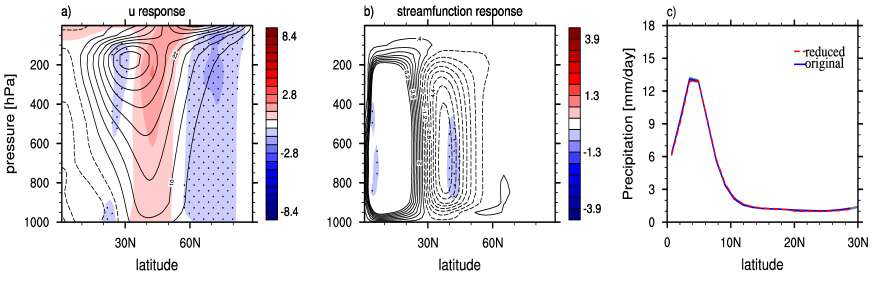
Figure 6: Same as Figure 2 but for the response to reduced $Z_{0m}$ in the extratropics only, for $|\phi|>20\degree$.

It should be noted that the magnitude of the extratropical $\overline{u}$ response (Figure 2a)—especially in the upper troposphere—is similar to the response to reduced Rayleigh drag discussed in Chen et al. (2007) (their figure 6c). In particular, the pattern of the response projects strongly onto the annular mode pattern, defined as the leading EOF of $\overline{u}$ (or surface pressure). While in Chen et al. (2007) the response to the reduced Rayleigh drag is purely extratropical, here the tropical circulation also responds to reduced $Z_{0m}$.

The ITCZ—defined as the maximum in $P$—generally coincides with the zero in $\Psi$, as long as $\Psi$ is not strongly asymmetric about the ITCZ (Bischoff and Schneider, 2015). The poleward shift of the ITCZ in response to the reduced $Z_{0m}$ can clearly be seen in Figure 2$c$.

The response of the ITCZ to the reduced $Z_{0m}$ at low flow speed is remarkably similar to the response discussed in Numaguti (1993) with fixed $Z_{0m}$. When he re-introduced the wind dependency to the bulk formula for $E$ (equation (1)) instead of fixing $|\Delta{\bf v}|$= 6 m s^-1, the total precipitation transitioned from having a single peak at the equator to having a double peak straddling the equator. The double ITCZ formed because $|\Delta{\bf v}|\approx 0$ at the equator implied that $E\approx 0$ there.

Figure 3: Zonal-mean temperature $\overline{T}$ [K] response to reduced $Z_{0m}$ in coloured shading (negative values are stippled). Contours show the original climatology ($10$ K spacing).

3.1 Other SST profiles

To check the robustness of the circulation response to reduced $Z_{0m}$, simulations forced by hemispherically-symmetric “Control” and “Flat” (figure 1$a$ in Neale and Hoskins (2000)) and hemispherically-asymmetric “Qobs10N” (as “Qobs” but with maximum in SST displaced $10\degree$N) SSTs are also performed. The circulation responses are shown in Figure 4. The different SST profiles produce distinct basic states, especially in the tropics (see discussion in Williamson et al. (2013)). Despite the magnitude being smaller (notice the smaller contour interval), it is clear from the figure that the responses are similar to that in Figure 2. Experience has shown that even under other forcings (i.e., other than the reduction in $Z_{0m}$), simulations forced by “Qobs” SST tend to exhibit a larger magnitude response compared to the simulations forced by the “Control” or “Flat” SSTs, which produce stronger and weaker HC, respectively. The reasons behind this will be discussed in a future paper. In what follows, the circulation response is elucidated only in the simulations forced by the “Qobs” SST profile.

Note that in the “Qobs10N” simulation, the HC return flow rises above the boundary layer at the equator and gradually crosses to the hemisphere with the SST maximum in the free troposphere (Figure 4$h$). This also occurs in the AMIP-type simulations (see Figures 13 and 14). Such behaviour can be associated with too weak a temperature gradient or too shallow a boundary layer depth at the equator (Pauluis, 2004). Consequently, two precipitation maxima are produced: one almost at the equator, where $\overline{v}$ changes sign in the lower troposphere, and the other poleward of the SST maximum where $\overline{v}$ changes sign in the upper troposphere.

$\begin{array}[]{ccc}\includegraphics[width=433.62pt]{FIG4a.pdf}\\ \includegraphics[width=433.62pt]{FIG4b.pdf}\\ \includegraphics[width=433.62pt]{FIG4c.pdf}\end{array}$

Figure 4: Same as Figure 2 but for the response to reduced $Z_{0m}$ in simulations forced by “Control” (top), “Flat” (middle) and “Qobs10N” (bottom) SSTs. Note the different contour interval than in Figure 2. In the “Qobs10N” case, the latitudinal range in the panels is centred at the equator.

3.2 Tropical energy fluxes as mediators of the response

Reducing $Z_{0m}$ affects both the tropical and the extratropical circulation (Figure 2). Therefore it is natural to ask if the zonal-mean circulation response arises from reducing $Z_{0m}$ in the tropics only, the extratropics only, or both. Because reducing $Z_{0m}$ affects both latent and sensible heat fluxes ($E$ and $H$, respectively) and surface stresses ($\boldsymbol{\tau}$) (equations 1-4), it is also natural to ask if the response is mediated through reduction of $Z_{0m}$ in $H$ and $E$ or in $\boldsymbol{\tau}$. In other words, is the response thermodynamically or dynamically initiated?

To address the first question, two aquaplanet simulations are performed where the reduction in $Z_{0m}$ is restricted only to latitudes ($\phi$) i) $|\phi|\leq\pm 20\degree$ and ii) $|\phi|>\pm 20\degree$. To address the second question, two additional simulations are performed where reduction in $Z_{0m}$ is applied only in the bulk formulation (equation 1) for i) $H$ and $E$ and ii) $\boldsymbol{\tau}$.

Figures 5 and 6 show the zonal-mean circulation response from the first set of simulations. By comparing the two figures with Figure 2, it is clear that the response—even in the mid-latitudes—is mediated from the tropics. This suggests the existence of a zonally-symmetric tropical-extratropical teleconnection, which is discussed in section 3.3.

Figures 7 and 8 show the zonal-mean circulation response from the second set of simulations. By comparing the two figures with Figure 2, it is clear that the total response is mostly thermodynamically mediated, i.e., through reducing $Z_{0m}$ in $H$ and $E$. Notably, the tropical circulation response to reducing $Z_{0m}$ in $\boldsymbol{\tau}$ is opposite to the total response; the HC upwelling region, the ITCZ, and the subtropical jet shift equatorward in this case. The equatorward shift of the ITCZ in response to reduction of $\boldsymbol{\tau}$ is a result of the wind-evaporation feedback (e.g. Neelin et al., 1987): The immediate response to reducing $\boldsymbol{\tau}$ at low flow speed is to accelerate the tropical near-surface winds. Because $E$ depends on the near-surface wind magnitude (equation 1), the increase in the tropical surface winds leads to the enhanced $E$ there. As a result, the HC strengthens (maximum in $\Psi$ at 500 hPa is $\approx$8% stronger), the ITCZ shifts equatorward (see section 3.3 for explanation) and the subtropical jet becomes stronger (region of positive anomaly in the upper troposphere equatorward of 20$\degree$N in Figure 8$a$). This is similar to the simulation in Numaguti (1993), in which the equatorial flow speed was artificially enhanced by setting $\Delta{\bf v}=6$ m s^-1 everywhere. However, the wind-evaporation feedback is weak in the simulations shown in Figure 2 because any increase in wind from reducing $Z_{0m}$ in $\boldsymbol{\tau}$ is compensated by the reduction of $Z_{0m}$ in the equation that prescribes $E$.

Note that the ITCZ is displaced further poleward in the simulation where $Z_{0m}$ is reduced for $E$ and $H$ only (cf. Figure 2$c$ with Figure 7$c$). This suggests that the wind-evaporation feedback acts to partially counteract the poleward displacement of the ITCZ in the total response (Figure 2). However, the full response is not linear to the reduction of $Z_{0m}$ in $\boldsymbol{\tau}$ and in $E$ and $H$ (i.e., the sum of the responses in Figures 7 and 8 is not the same as the response in Figure 2). Interestingly, the mid-latitude westerlies shift poleward in response to reduced $\boldsymbol{\tau}$ (Figure 8$a$). Thus it is possible that the mechanism discussed in Chen et al. (2007) that relies on the increase in wave phase speeds and the resulting poleward shift of the critical latitude region is playing some role here.

Figure 5: Same as Figure 2 but for the response to reduced $Z_{0m}$ in the tropics only, for $|\phi|<20\degree$.

Figure 7: Same as Figure 2 but for the response to reduced $Z_{0m}$ in the bulk formulation for latent and sensible heat fluxes only.

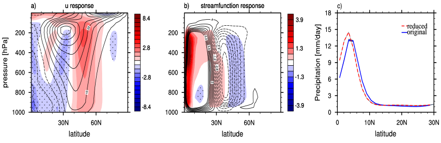
Figure 8: Same as Figure 2 but for the response to reduced $Z_{0m}$ in the bulk formulation for surface stress only.

Given that $Z_{0m}$ is reduced at low flow speed only, it is perhaps not surprising that tropical $E$ and $H$ play a dominant role in the total response as the extratropical surface winds are directly only weakly affected. However, in simulations where $Z_{0m}$ is unrealistically uniformly reduced by a factor of 0.5 to affect all flow speeds, the response is nearly identical to that in Figure 2 (not shown). This suggests that the reduction of $Z_{0m}$ at low flow speed—and especially the effect of this reduction on $E$ and $H$—is instrumental to the response. When $Z_{0m}$ is reduced by a factor of 0.5 in the bulk formulation for $\boldsymbol{\tau}$ only, a stronger extratropical response than in Figure 8 is produced; the westerlies on the poleward flank of the mid-latitude jet strengthen and there is an accompanying increase in wave phase speed (not shown). Thus, if $Z_{0m}$ in $\boldsymbol{\tau}$ (but only in $\boldsymbol{\tau}$) is substantially reduced at all flow speeds, the mechanism discussed in Chen et al. (2007) is likely to operate. However, different from Chen et al. (2007), a strong tropical response is present in that case; the HC strengthens and the ITCZ shifts equatorward as a result of the wind-evaporation feedback.

Finally, it is worth emphasizing that in simulations forced by other SST profiles (see Figure 4) the tropical energy fluxes are also instrumental in the total response (not shown).

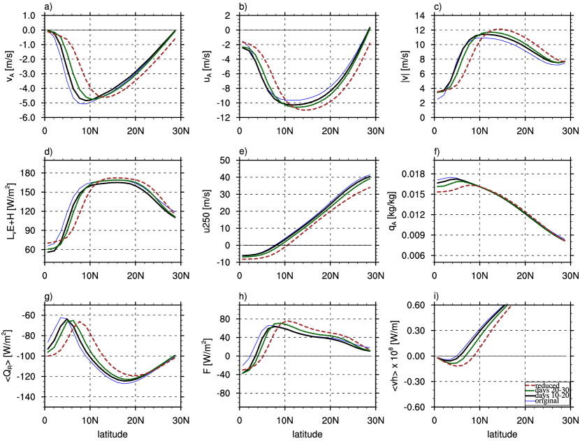
Figure 9: (a): The lowest model level meridional wind $v_{A}$. (b) The lowest model level zonal wind $u_{A}$. (c) $|\Delta{\bf v}|=\text{max}(1,\sqrt{u_{A}^{2}+v_{A}^{2}})$. (d): $L_{v}E+H$. (e): Zonal wind at 250 hPa. (f): The lowest model level specific humidity $\overline{q}_{A}$. (g): $\langle Q_{R}\rangle$. (h): Net moist static energy input ${\cal F}$. (i): Moist static energy flux $\langle\overline{vh}\rangle$. The fields from the equilibrated original $Z_{0m}$ simulation are shown in solid lines and from the reduced $Z_{0m}$ simulation in dashed lines. The fields averaged over $t=$[10:20] days are shown in thick lines and over $t=$[20:30] days in dotted lines.

3.3 Understanding the circulation response

If $Z_{0m}$ is reduced, a potential null hypothesis would be that the surface winds would accelerate to maintain the same $\boldsymbol{\tau}$. The increase in surface winds would counteract the decrease in $C_{E}$ and $C_{H}$ leaving $E$ and $H$ unchanged (see equation (1)). However, the null hypothesis is clearly invalid in this study, where the reduction in tropical $E$ and $H$ is crucial in initiating the response. More importantly, the acceleration of meridional surface winds implied by the null hypothesis is inconsistent with Ekman balance, because unchanged $\boldsymbol{\tau}$ implies unchanged Ekman pumping (i.e. in a zonally-symmetric case and employing an equatorial $\beta$-plane approximation the Ekman pumping $w_{E}\sim-\frac{\partial\rho\overline{v_{E}}}{\partial y}\sim-\frac{1}{\beta y}\frac{\partial\overline{\tau}_{x}}{\partial y}$, where $v_{E}$ is the meridional wind in the Ekman layer) and hence unchanged meridional winds in the boundary layer. Therefore, something else has to happen in the reduced $Z_{0m}$ simulations.

To examine how the circulation response is established, a 50 ensemble member switch-on simulation is performed. In the simulation, the reduced $Z_{0m}$ is suddenly switched on in the bulk formulation for all the fluxes at $t=10$ days. Each member is initialized from a random point in the equilibrated original $Z_{0m}$ simulation. Figure 9 shows tropical zonal-mean distributions of fields, important for understanding the adjustment, at different stages after the switch-on.

When the reduced $Z_{0m}$ is switched on, the surface meridional wind ($v_{A}$) weakens initially in the tropics (cf. solid line with thick line in panel $a$) as a result of the weaker Ekman drag from $\tau_{x}$ that drives $v_{A}$. The initial decrease in $\tau_{x}$ can be seen in Figure 12$a$ (cf. solid line with dashed line). The reduction in $\tau_{x}$ is evidently more important than the decrease in $\tau_{y}$ and in contrast, the initial response in surface zonal wind ($u_{A}$) is a strengthening near the equator and at $10\degree$N$\,<\phi<20\degree$N (panel $b$). Hence, the initial response is a reduction in $L_{v}E+H$ everywhere (panel $d$), because $|\Delta{\bf v}|=\text{max}(1,\sqrt{u_{A}^{2}+v_{A}^{2}})$ (panel $c$) does not increase enough to compensate for the decrease in $Z_{0m}$. The latter is the result of the weakening of $v_{A}$ just discussed. The inevitable consequence of reduced $L_{v}E+H$ is to dry and cool the tropics. This can be seen in Figure 3, where the cooling (growing with altitude because of the drying) spreads upward in the deep tropics and poleward in the tropical mid to upper troposphere.

A cooler tropical mid to upper troposphere implies a weakened subtropical temperature gradient and thus a weakened equatorial flank of the subtropical jet (panel $e$, also Figure 2$a$)—in analogy with the La Ni$\tilde{\text{n}}$a phase of ENSO variability (e.g. Seager et al. (2003) and Lu et al. (2008)). Because the tropical meridional temperature gradient is weaker in the reduced $Z_{0m}$ simulation, the weaker jet follows from thermal wind balance. The HC mass flux is also weaker as a weaker HC can now maintain uniform temperatures in the tropics (e.g. Schneider, 2006). Thus another way of understanding the weakened subtropical jet is weakened angular momentum transport by the HC.

A weakened equatorial flank of the subtropical jet implies a poleward shift of the critical latitudes in the subtropics. The critical latitude is the region where the wave phase speed $c$ closely matches the mean flow speed $\overline{u}$. It is the region where the Rossby waves, generated by the near-surface baroclinic instability, break and deposit easterly momentum (Randel and Held, 1991). The poleward shift in the critical latitude in response to reduction in $Z_{0m}$ can be seen in Figure 10, which shows the equilibrated eddy momentum flux convergence spectra as a function of angular phase speed ($c_{A}=c/\cos\phi$) and $\phi$ at 250 hPa. The figure bears a marked resemblance to figure 9 in Lu et al. (2008) for the El Ni$\tilde{\text{n}}$o minus La Ni$\tilde{\text{n}}$a ENSO variability, taking into account the sign reversal. In particular, in the reduced $Z_{0m}$ simulation there is a systematic poleward shift of the critical latitude for waves of all $c_{A}$ and a poleward shift of the whole eddy momentum flux convergence spectrum, with a characteristic convergence-divergence-convergence tripole pattern in the response.

It is clear that the weaker subtropical jet leads the poleward critical latitude shift, because an initial poleward shift of the critical latitudes would strengthen rather than weaken the winds on the equatorial flank of the jet (because of less wave drag there). This poleward critical latitude shift explains the poleward shift in the HC terminus, and also acts to weaken the core of the jet.

Finally, the tropical cooling also reduces baroclinicity in the subtropical latitudes, reducing the baroclinic eddy generation as reflected in Figure 11, which shows the quasi-geostrophic EP flux diagnostics (Edmon et al., 1980) for the original $Z_{0m}$ climatology in ($a$) and the response in ($b$). In the original $Z_{0m}$ simulation the EP flux, which represents wave activity propagation, resembles the classic scenario with upward wave propagation in the lower and middle troposphere and mostly equatorward wave propagation aloft. The response in ($b$) shows a reduced EP flux convergence in mid-latitudes (the red patch in Figure 11$b$), and thus less deceleration, which accounts for the strengthened poleward flank of the subtropical jet. Together with the critical latitude shift discussed above, this explains the tripole eddy momentum flux convergence pattern and the poleward jet shift.

To further support the mechanistic chain of events just discussed and to determine the timescales involved in the adjustment, it is instructive to examine how the Ekman and zonal momentum balances are restored following the switch-on. Figure 12 shows the adjustment of Ekman and momentum balance terms to their reduced $Z_{0m}$ equilibrium counterparts at 7$\degree$N (panel $b$) and at 50$\degree$N (panel $c$). In order to more easily interpret the responses in panels ($b$) and ($c$), the evolution of zonal-mean $\tau_{x}$ during the adjustment is shown for reference in panel ($a$). The meridional momentum flux convergence and $f\overline{v}$ (integrated over the boundary layer) closely follow the spatial distribution of $\tau_{x}$.

Figure 10: Eddy momentum flux convergence spectra $\times 10^{-7}$ [m s^-2] at 250 hPa for the original $Z_{0m}$ simulation (in coloured shading, negative values are stippled) and the response to reduced $Z_{0m}$ (in contours, negative values are dashed). The solid and dashed lines show $\overline{u}/\cos\phi$ [m s^-1] for the original and the reduced $Z_{0m}$ simulations, respectively. The eddy momentum flux cospectrum is calculated following Hayashi (1971) and Randel and Held (1991) before taking the divergence.

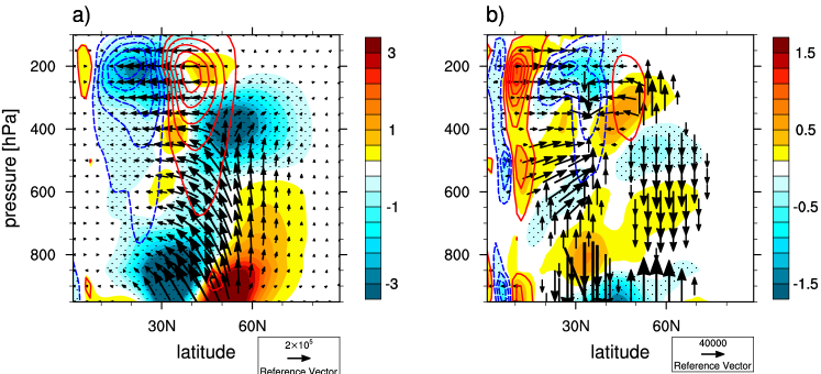
Figure 11: Eliassen Palm fluxes [m^-2 s^-2] (vectors), their divergence $\times 10^{9}$ [m s^-2] (in coloured shading, negative values are stippled) and eddy momentum flux convergence (dashed and solid contours). ($a$) The original $Z_{0m}$ climatology. ($b$) The response to reduced $Z_{0m}$. Note both the equatorward and poleward wave propagation in ($a$).

Figure 12: (a): The zonal mean zonal surface stress $\overline{\tau}_{x}$ at different stages of the adjustment. (b-c) The adjustment of Ekman and momentum balance to the new equilibrium obtained for reduced $Z_{0m}$ at (b) 7$\degree$N and (c) 50$\degree$N: total meridional momentum flux convergence (thin line); eddy meridional momentum flux convergence (dotted line); mean meridional momentum flux convergence (thick line); zonal surface stress (dashed dotted line); $f\overline{v}_{E}$ (dotted line). Panels (b) and (c) show deviations from the final, reduced $Z_{0m}$ equilibrium values.

After the switch-on, $\tau_{x}$ and $f\overline{v}$ track each other extremely closely (cf. dotted line with dash dotted line in panels ($b$) and ($c$)), showing that Ekman balance is restored almost instantly and holds throughout the adjustment process. While the tropical momentum flux convergence (MFC) also follows $\tau_{x}$ relatively closely, there is a slight imbalance that reflects the lack of equilibrium (cf. solid line with dotted line). The tropical MFC adjustment is mainly occurring through the mean MFC term (thick line). This is a direct consequence of the weakened subtropical temperature gradient effected by reduced $L_{v}E+H$. In contrast, the tropical eddy MFC (dotted line) only starts to respond $\approx$ 15 days after the switch-on. This shows that the eddy changes respond to the mean flow changes, rather than vice-versa. In the extratropics, the MFC and $\tau_{x}$ only start to respond $\approx$ 30 days after the switch-on (panel $c$). In summary, the upper tropospheric eddy MFC in the subtropics responds to the mean changes in the tropics and the extratropical changes (reflecting changes in baroclinic generation) occur later. It is important to understand that the mechanism behind the poleward midlatitude jet shift proposed in this study is initiated by the tropical mean flow changes. In contrast, the mechanism behind the poleward jet shift in Chen et al. (2007) in response to reduced Rayleigh drag is initiated by the extratropical MFC changes.

3.4 ITCZ shift

The arguments in section 3.3 explain the HC weakening and the poleward shift of the mid-latitude westerlies and the subtropical descent region. However, the poleward shift of the ITCZ in these simulations remains to still be elucidated. The moist static energy budget provides a useful framework for understanding the poleward ITCZ shift. Neglecting a relatively small contribution from the atmospheric kinetic energy, the vertically-integrated, zonal-mean moist static energy budget in a steady state is

$$\partial_{\phi}\langle\overline{vh}\rangle=\langle Q_{R}\rangle+L_{v}E+H\equiv\cal{F},$$ (6)

where $\langle.\rangle$ denotes a mass-weighted vertical integral over the atmospheric columns; $\overline{(.)}$ denotes zonal and temporal mean; $h=c_{p}T+\Phi+L_{v}q$ is the moist static energy, where $\Phi$ is the geopotential height, $L_{v}$ is the latent heat of vaporization, and $Q_{R}$ is the net radiative flux. The reader is referred to Neelin and Held (1987) for the derivation of equation (6).

Equation (6) states that the divergence of the moist static energy flux $\langle\overline{vh}\rangle$ is balanced by the net moist static energy input to the atmosphere $\cal{F}$. As long as the gross moist stability is positive, $\langle\overline{vh}\rangle$ has the same sign as the mass flux in the upper branch of the HC (see e.g., discussion in Bischoff and Schneider (2015) in their Appendix 2). Therefore, the principal quantity controlling the position of the HC is the net supply of moist static energy, which is a small difference between the net supply by latent and sensible heat fluxes $L_{v}E+H$ and the energy loss by radiative cooling $\langle Q_{R}\rangle$. In particular, a small fractional change in $L_{v}E$ and $H$ can cause a large change in the energy balance of the HC.

As long as the latitude where $\overline{v}$ changes sign does not vary strongly with height (as in the hemispherically symmetric simulations in this study), the HC upwelling region and the ITCZ are located at the latitude where $\langle\overline{vh}\rangle=0$ — i.e., at the “energy flux equator” (Kang et al., 2008, 2009). To understand the ITCZ shift it is instructive to examine the evolution of $\cal F$ and $\langle\overline{vh}\rangle$ during the adjustment in Figures 9$h$ and 9$i$. Note that $\langle\overline{vh}\rangle$ is the latitudinal integral of $\cal F$, and $\langle\overline{vh}\rangle=0$ at the equator in the hemispherically-symmetric case discussed here.

The initial reduction in $L_{v}E+H$ reduces $\cal F$ in the tropics (cf. solid line with thick and dotted lines in panel $h$) and thus increases the latitude at which $\langle\overline{vh}\rangle$ passes through zero (panel $i$). Thus the ITCZ is predicted to shift poleward. As the ITCZ shifts poleward, the surface easterlies and the latitude where $v_{A}$ changes sign are pushed poleward to maintain Ekman balance. This leads to a decrease in $|\overline{\triangle{\bf v}}|$ on either side of the equator (Figure 9$c$) and a concomitant decrease in $L_{v}E+H$ there (Figure 9$d$). Additionally, the minimum in the outgoing longwave radiation shifts poleward and hence modifies the $\langle Q_{R}\rangle$ distribution pushing the maximum in $\langle Q_{R}\rangle$ at $5\degree$N poleward (Figure 9$g$). Hence, the energy flux equator moves further poleward than initially. As the ITCZ settles to its final latitude, $\Delta q$ and $\Delta\theta$ begin to increase to restore $L_{v}E+H$ ($\Delta q$ increase is reflected in $q$ change in Figure 9$f$). Despite this the tropical atmosphere remains cooler than in the original $Z_{0m}$ simulation as the same flux can be achieved with a reduced $Z_{0m}$ if the vertical gradient increases.

4 Results: AMIPsst and AMIPsom simulations

How robust is the zonal-mean circulation response to reduction in $Z_{0m}$ at low flow speed? To address this, sensitivity experiments are performed under an AMIP-type setup with both prescribed SSTs (i.e. AMIPsst) and with a mixed layer slab ocean lower boundary condition (i.e. AMIPsom). Recall that the AMIP setup includes the seasonal cycle and the full complexity of atmosphere-ice-land-ocean interaction.

Figures 13 and 14 show the circulation response for December-January-February (DJF) to reduced $Z_{0m}$ at low flow speed in the AMIPsst and AMIPsom simulations, respectively. Similar responses occur also in other seasons (not shown). Despite the weaker response compared to the aquaplanet simulations, it is clear from the figures that the zonal-mean circulation response to reduced $Z_{0m}$ carries over to more complex setups. In particular, the response in Figures 13 and 14 closely resembles the response in the aquaplanet simulation (with hemispheres reversed) forced by the hemispherically-asymmetric “Qobs10N” SST (see Figure 4, bottom row). Given that the sensitivity is not substantially compromised in the presence of the seasonal cycle and the full complexity of atmosphere-ice-land-ocean interaction, the aquaplanet framework appears to be a fruitful avenue for understanding the zonal-mean circulation response in more complex models.

Note that the peak in the zonal-mean precipitation maximum in the summer hemisphere weakens but does not move poleward in response to reduced $Z_{0m}$ in both experiments. This is because the reduction in the net equatorial energy input is too small to push the ITCZ poleward. Note also the presence of a second precipitation maximum in the winter hemisphere. As discussed earlier, this is because the latitude where $\overline{v}$ changes sign is not barotropic, with the HC return flow rising above the boundary layer at the equator and gradually crossing to the hemisphere with the SST maximum in the free troposphere (see Figures13$b$ and 14$b$). For a more detailed view, latitude-longitude cross sections of the total precipitation response in the AMIPsst and AMIPsom experiments are shown in Figure 15. In the figure, the largest precipitation response occurs over the western and central Pacific and the Indian ocean.

Figure 13: Same as Figure 2 but for the response to reduced $Z_{0m}$ in the AMIP-type simulations for DJF with fixed SSTs.

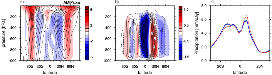
Figure 14: Same as Figure 13 but with slab ocean mixed layer lower boundary condition.

Figure 15: Total precipitation response [mm day^-1] (coloured shading, negative values are stippled) for DJF in cylindrical-equidistant projection for the AMIP-type simulations without ($a$) and with ($b$) a slab ocean mixed layer lower boundary condition. The original $Z_{0m}$ climatology is overlaid in gray contours.

Interestingly, while the circulation sensitivity to reduced $Z_{0m}$ is similar in the AMIPsst and AMIPsom simulations, the global temperature response is different; the tropospheric temperature warms globally in the AMIPsom experiments. However, the temperature response in the slab ocean simulations appears to be rather sensitive to the internal ocean heat flux and mixed layer depth specification and is therefore not robust. Detailed investigation into this difference between the AMIPsst and AMIPsom simulations is, however, outside the scope of this study.

5 Summary and Conclusion

This study explored the sensitivity of the zonal-mean circulation to reduction in air-sea momentum roughness $Z_{0m}$ at low flow speed in CAM3 under three setups: 1) Aquaplanet forced by zonally-symmetric time-invariant SST, 2) AMIP-type forced by seasonal SST and sea ice distributions and including the full complexity of atmosphere-ice-land-ocean interaction, and 3) AMIP-type with a mixed layer slab ocean lower boundary condition. In all three setups the circulation response to reduced $Z_{0m}$ at low flow speed is significant and resembles the La Ni$\tilde{\text{n}}$a minus El Ni$\tilde{\text{n}}$o differences in ENSO variability (Seager et al., 2003; Lu et al., 2008; Sun et al., 2013) with; i) a poleward shift of the mid-latitude westerlies extending all the way to the surface; ii) a weak poleward shift of the subtropical descent region; iii) a weakening of the HC, generally also accompanied by a poleward shift of the ITCZ and the tropical surface easterlies. Mechanism-denial experiments in the aquaplanet framework pinned down the reduction of tropical latent and sensible heat fluxes (effected by reducing $Z_{0m}$ at low flow speed) as the main mediators of the circulation response. The mechanisms behind the circulation response were also elucidated in the aquaplanet framework with an ensemble of reduced $Z_{0m}$ switch-on simulations.

The decrease in the tropical latent and sensible heat fluxes into the atmosphere cools the tropical troposphere (especially in the mid and high altitudes) and reduces the meridional temperature gradient there. As a result the HC weakens and, if the reduction in the energy fluxes is large enough (as in the aquaplanet simulations with “Qobs” SST profile), the upwelling region and the associated ITCZ shift poleward. The tropical circulation response is instrumental for the extratropical circulation response. In particular, a weakened HC is consistent with a weakened subtropical jet. The weakened jet shifts the upper tropospheric critical latitude region poleward on the equatorward flank of the subtropical jet. Importantly, the surface baroclinicity is also weakened on the equatorward flank of the midlatitude jet as a result of weaker meridional temperature gradients in the subtropics. Both the shift in the critical latitude and the reduced baroclinic eddy forcing result in a tripole EP flux divergence anomaly in the upper troposphere that induces a poleward shift in the mid-latitude jet and the HC terminus.

A salient point of this study is that relatively small changes in the parameterization parameters, within the observational constraints, can lead to a large response in the circulation. Here only surface layer parameter sensitivity was explored and in one GCM only. It is possible that similar changes to the surface layer scheme in GCMs other than CAM3 produce a different circulation response. For example, the interaction with other parameterizations might be different; Numaguti (1993) found that the ITCZ moved equatorward (rather than poleward) in response to reduced (and negative) net moist static energy input to the equator, because the equatorward transport of the latent energy surpassed the poleward transport of the dry static energy (resulting in negative gross moist stability in the tropics) in the simulations with a dry convective adjustment scheme. Thus, delineating the interaction of surface layer parameterizations with convection and cloud parameterizations deserves further study. It is also conceivable that the changes to the momentum budget via reduction in surface stresses play a stronger role in the total response in other GCMs; for example, the wind-evaporation feedback potentially could overcome the weakening of the HC and the poleward ITCZ shift.

As is shown here, uncertainties in surface process parameterizations are likely to contribute to the systematic errors in GCM simulations together with cloud and convective parameterizations, which are often singled out as sole culprits. Furthermore, it is plausible that reasonable changes in other parameterization parameters can lead to as large a circulation response as observed here. Therefore, it is important to understand such parameter sensitivities in order to delineate non-robust circulation responses to climate forcing (e.g. Stevens and Bony, 2013; Shepherd, 2014).

References

- Barnes and Hartmann (2010) Barnes EA, Hartmann DL. 2010. Influence of eddy-driven jet latitude on North Atlantic jet persistence and blocking frequency in CMIP3 integrations. GRL, 37. doi:10.1029/2010GL045700
- Bischoff and Schneider (2015) Bischoff T, Schneider T. 2015. The equatorial energy balance, ITCZ position, and double ITCZ bifurcations. J. Clim., doi: 10.1175/JCLI-D-15-0328.1
- Blackburn et al. (2013) Blackburn, M., Williamson DL, Nakajima K, and co-authors. 2013. The aqua-planet experiment (APE): CONTROL SST simulation. J. Met. Soc. Japan, Series 2, 91A, 17–56. doi:10.2151/jmsj.2013-A02
- Boville (2006) Boville BA, Rasch PJ, Hack JJ, McCaa JR. 2006. Representation of clouds and precipitation processes in the Community Atmosphere Model version 3 (CAM3). J. Clim., 19, 2184–2198. doi:10.1175/JCLI3749.1
- Chen et al. (2007) Chen G, Held IM, Robinson WA. 2007. Sensitivity of the latitude of the surface westerlies to surface friction. J. Atmos. Sci., 64, 2899–2915. doi:10.1175/JAS3995.1
- Collins et al. (2006) Collins WD, Rasch PJ, Boville BA, Hack JJ, McCaa JR, Williamson DL, Briegleb PB, Bitz CM, Lin S-J, Zhang M. 2006. The formulation and atmospheric simulation of the Community Atmosphere Model version 3 (CAM3). J. Climate, 19, 2144–2161. doi:10.1175/JCLI3760.1
- Edmon et al. (1980) Edmon Jr HJ, Hoskins BJ, McIntyre ME. 1980. Eliassen-Palm cross sections for the troposphere. J. Atmos. Sci., 37, 2600–2616. doi:10.1175/1520-0469(1980)037<2600:EPCSFT>2.0.CO;2
- Edson (2008) Edson J. 2009. ‘Review of air-sea transfer processes, paper presented at ECMWF Workshop 2008 on Ocean-Atmosphere Interactions’. Reading, England.
- Gates et al. (1999) Gates WL, Boyle JS, Covey C, Dease CG, Doutriaux CM, Drach RS, Fiorino M, et al. 1999. An overview of the results of the Atmospheric Model Intercomparison Project (AMIP I). Bull. Amer. Meteor. Soc. 80, no1, 29–55. doi:10.1175/1520-0477(1999)080<0029:AOOTRO>2.0.CO;2
- Garfinkel et al. (2011) Garfinkel CI, Molod AM, Oman LD, Song I-S. 2011, Improvement of the GEOS-5 AGCM upon updating the air-sea roughness parameterization.GRL 38, L18702, doi:10.1029/2011GL048802.
- Garfinkel et al. (2013) Garfinkel CI, Oman LD, Barnes EA, Waugh DW, Hurwitz MH, Molod AM. 2013. Connections between the Spring Breakup of the Southern Hemisphere Polar Vortex, Stationary Waves, and Air-Sea Roughness. J. Atmos. Sci., 70, 2137–2151. doi:10.1175/JAS-D-12-0242.1
- Hack et al. (1994) Hack JJ, Boville BA, Kiehl JT, Rasch PJ, Williamson DL. 1994. Climate statistics from the National Center for Atmospheric Research community climate model CCM2. JGR: Atmospheres, 99, 20785–20813. doi:10.1029/94JD01570
- Hayashi (1971) Hayashi Y. 1971. A generalized method of resolving disturbances into progressive and retrogressive waves by space Fourier and time cross-spectral analysis, J. Meteorol. Soc. Jpn., 49, 125–128.
- Held and Suarez (1994) Held IM, Suarez MJ. 1994. A proposal for the intercomparison of the dynamical cores of atmospheric general circulation models, Bull. Amer. Meteor. Soc., 75, 1825–1830. doi:10.1175/1520-0477(1994)075<1825:APFTIO>2.0.CO;2
- Helfand and Schubert (1995) Helfand HM, Schubert SD. 1995. Climatology of the simulated Great Plains low-level jet and its contribution to the continental moisture budget of the United States. J. Climate, 8, 784–806. doi:10.1175/1520-0442(1995)008<0784:COTSGP>2.0.CO;2
- Holtslag and Boville (1993) Holtslag AAM, Boville BA. 1993. Local versus nonlocal boundary-layer diffusion in a global climate model. J. Climate, 6, 1825–1842. doi:10.1175/1520-0442(1993)006<1825:LVNBLD>2.0.CO;2
- Hwang and Frierson (2013) Hwang Y-T, Frierson DMW. 2013. Link between the double-Intertropical Convergence Zone problem and cloud biases over the Southern Ocean. Proc. Natl. Acad. Sci., 110, 4935–4940, doi:10.1073/pnas.1213302110
- Kang et al. (2009) Kang SM, Frierson DM, Held IM. 2009. The tropical response to extratropical thermal forcing in an idealized GCM: The importance of radiative feedbacks and convective parameterization. J. Atmos. Sci., 66, 2812–2827. doi:10.1175/2009JAS2924.1
- Kang et al. (2008) Kang SM, Held IM, Frierson DM, Zhao M. 2008. The response of the ITCZ to extratropical thermal forcing: Idealized slab-ocean experiments with a GCM. J. Climate, 21, 3521–3532. doi:10.1175/2007JCLI2146.1
- Large et al. (1994) Large WG, McWilliams JC, Doney SC. 1994. Oceanic vertical mixing: A review and a model with a nonlocal boundary layer parameterization. Reviews of Geophysics, 32, 363–404. doi:10.1029/94RG01872
- Large and Pond (1982) Large WG, Pond S. 1982. Sensible and latent heat flux measurements over the ocean. J. Phys. Oceanography, 12, 464–482. doi:10.1175/1520-0485(1982)012<0464:SALHFM>2.0.CO;2
- Lee et al. (2008) Lee MI, Suarez MJ, Kang IS, Held IM, Kim D. 2008. A moist benchmark calculation for atmospheric general circulation models. J. Clim., 21, 4934–4954. doi:10.1175/2008JCLI1891.1
- Lu et al. (2008) Lu J, Chen G, Frierson DM. 2008. Response of the zonal mean atmospheric circulation to El Nio versus global warming. J. Clim., 21, 5835–5851. doi:10.1175/2008JCLI2200.1
- Miller et al. (1992) Miller MJ, Beljaars ACM, Palmer TN. 1992. The sensitivity of the ECMWF model to the parameterization of evaporation from the tropical oceans. J. Clim., 5, 418–434. doi:10.1175/1520-0442(1992)005<0418:TSOTEM>2.0.CO;2
- Monterey and Levitus (1997) Monterey G, Levitus S, 1997, Seasonal Variability of Mixed Layer Depth for the World Ocean. NOAA Atlas NESDIS 14, U.S. Gov. Printing Office, Wash., D.C., 96 pp. 87 figs.
- Neale and Hoskins (2000) Neale RB, Hoskins BJ. 2000. A standard test for AGCMs including their physical parametrizations: I: The proposal. Atmospheric Science Letters, 1, 101–107. doi:10.1006/asle.2000.0022
- Neelin and Held (1987) Neelin JD, Held IM. 1987. Modeling tropical convergence based on the moist static energy budget. Mon. Wea. Rev. 115, 3–12. doi:10.1175/1520-0493(1987)115<0003:MTCBOT>2.0.CO;2
- Neelin et al. (1987) Neelin JD, Held IM, Cook KH. 1987. Evaporation-wind feedback and low-frequency variability in the tropical atmosphere. J. Atmos. Sci., 44, 2341-2348. doi:10.1175/1520-0469(1987)044<2341:EWFALF>2.0.CO;2
- Numaguti (1993) Numaguti A. 1993. Dynamics and energy balance of the Hadley circulation and the tropical precipitation zones: Significance of the distribution of evaporation. J. Atmos. Sci., 50, 1874–1887. doi:10.1175/1520-0469(1993)050<1874:DAEBOT>2.0.CO;2
- Pauluis (2004) Pauluis O. 2004. Boundary layer dynamics and cross-equatorial Hadley circulation. J. Atmos. Sci., 61, 1161–1173. doi:10.1175/1520-0469(2004)061<1161:BLDACH>2.0.CO;2
- Randel and Held (1991) Randel WJ, Held IM. 1991. Phase speed spectra of transient eddy fluxes and critical layer absorption, J. Atmos. Sci., 48, 688–697.
- Schneider (2006) Schneider T. 2006. The general circulation of the atmosphere. Annu. Rev. Earth Planet. Sci., 34, 655–688. doi:10.1146/annurev.earth.34.031405.125144
- Seager et al. (2003) Seager R, Harnick N, Kushnir Y, Robinson W, Miller J, 2003, Mechanisms of hemispherically symmetric climate variability. J. Clim., 16, 2960–2978. doi:10.1175/1520-0442(2003)016<2960:MOHSCV>2.0.CO;2
- Shepherd (2014) Shepherd TG. 2014. Atmospheric circulation as a source of uncertainty in climate change projections. Nature Geoscience. 7, 703–708. doi:10.1038/ngeo2253
- Simpson et al. (2013) Simpson IR, Shepherd TG, Hitchcock P, Scinocca JF. 2013. Southern annular mode dynamics in observations and models. Part II: Eddy feedbacks.J. Clim., 26, 5220–5241. doi:10.1175/JCLI-D-12-00348.1
- Stevens and Bony (2013) Stevens B, Bony S. 2013. What are climate models missing? Science, 340, 1053–1054. doi: 10.1126/science.1237554
- Sun et al. (2013) Sun L, Chen G, Lu J. 2013. Sensitivities and mechanisms of the zonal mean atmospheric circulation response to tropical warming.J. Atmos. Sci., 70, 2487–2504.doi:10.1175/JAS-D-12-0298.1
- Williamson (2013) Williamson DL. 2013. Dependence of APE simulations on vertical resolution with the Community Atmospheric Model, version 3. J. Met. Soc. Japan, 91, 231–242. doi:10.2151/jmsj.2013-A08
- Williamson (2008) Williamson DL. 2008. Convergence of aqua-planet simulations with increasing resolution in the Community Atmospheric Model, Version 3. Tellus A, 60, 848–862.
- Williamson et al. (2013) Williamson DL, Blackburn M, Nakajima K, and co-authors. 2013. The Aqua-Planet Experiment (APE): Response to changed meridional SST profile. J. Met. Soc. Japan, Series 2, 91A, 57–89, doi:10.2151/jmsj.2013-A03
- Yelland et al. (1998) Yelland MJ, Moat BI, Taylor PK, Pascal RW, Hutchings J, Cornell VC. 1998, Wind stress measurements from the open ocean corrected for airflow distortion by the ship, J. Phys. Oceanogr., 28, 1511–1526, doi:10.1175/1520-0485(1998)028<1511:WSMFTO>2.0.CO;2
- Zhang and McFarlane (1995) Zhang GJ, McFarlane NA. 1995. Sensitivity of climate simulations to the parameterization of cumulus convection in the Canadian Climate Centre general circulation model. Atmosphere-Ocean, 33, 407–446. doi:10.1080/07055900.1995.9649539
- Zhang (2003) Zhang M, Lin W, Bretherton CS, Hack JJ, Rasch PJ. 2003. A modified formulation of fractional stratiform condensation rate in the NCAR Community Atmospheric Model (CAM2). JGR: Atmospheres, 108, ACL-10. doi:10.1029/2002JD002523