A/B Testing of Auctions

Abstract

For many application areas A/B testing, which partitions users of a system into an A (control) and B (treatment) group to experiment between several application designs, enables Internet companies to optimize their services to the behavioral patterns of their users. Unfortunately, the A/B testing framework cannot be applied in a straightforward manner to applications like auctions where the users (a.k.a., bidders) submit bids before the partitioning into the A and B groups is made. This paper combines auction theoretic modeling with the A/B testing framework to develop methodology for A/B testing auctions. The accuracy of our method is directly comparable to ideal A/B testing where there is no interference between A and B. Our results are based on an extension and improved analysis of the inference method of Chawla et al. (6).

1 Introduction

A common method in the practice of large scale auction design, e.g., in auctions placing advertisements on online media and Internet search engines, is A/B testing. In A/B testing, the auction house is running an incumbent mechanism A, and would like to determine if a novel mechanism B obtains higher revenue. This is done by splitting the traffic so that most of it goes to A and some of it, e.g., five to ten percent, goes to B. An issue with this approach is that if the bidders are unaware of which mechanism their bid will be considered in, the bid equilibrium is neither for A nor B but for a mechanism C that is a convex combination of A and B.

A miscalculation sometimes performed in practice is to consider and compare average revenue from A (resp. B) from the times when A (resp. B) is run. This miscalculation is equivalent to simulating A on the bids in C and can often give the opposite conclusion; e.g., if A and B are one- and two-unit highest-bids-win pay-your-bid auctions, respectively, then B will always appear in this miscalculation to have higher revenue. For a fixed set of bids, a pay-your-bid mechanism’s revenue is monotone in its allocation probabilities. Of course, in equilibrium, increased allocation probabilities can cause reduced revenue as bidders may lower their bids.

We present an A/B testing method that applies generally to the position auction model popularized by the Varian (24) and Edelman et al. (12) analyses of auctions for sponsored search and now a fundamental model for the study of auction theory; e.g., see Hartline (17). To revisit the example auction scenario above, notice that the mechanism C, namely the 50–50 convex combination of one- and two-unit auctions, is mathematically equivalent to a position auction with weights 1 and 0.5 for the top two slots respectively, and zero for all remaining slots. Mechanisms A and B are also position auctions. More generally, a position auction is defined by a decreasing sequence of weights, bidders are assigned to positions in decreasing order of bids, and payments are charged. Typical payment rules are “generalized first price” and “generalized second price”; the former requires bidders to pay their weighted bid, whereas the latter requires bidders to pay the weighted bid of the next highest bidder. (Unfortunately, for reasons we describe subsequently, our methods do not apply to the generalized second price position auction.) Position auctions with exogenously given weights are the standard model of auction for selling advertisements on Internet search engines. In this application, the weights correspond to the probability that the ad in each position on the search results page will be clicked on (and payments are scaled by weights because bidders only pay if they are clicked on).

Chawla et al. (6) developed an estimator for the revenue of one position auction (A or B) from the bids of another (C). This estimator is a simple weighted order statistic of the distribution of equilibrium bids in C. To estimate the revenue of B (analogously for A):

1. for any number $N$, the evaluation of a formula based on the definition of B and C gives $N$ weights, and,

2. given a sorted list of $N$ i.i.d. samples from the bid distribution for C, the estimated revenue of B is the weighted average of these bids.

This method of estimation compares favorably to ideal A/B testing, where the bids in A are in equilibrium for A and revenue can be estimated by simple averaging, respectively for B.

Our model of A/B testing is especially applicable to the following generalization of the classical problem with fixed position weights. Consider the problem Google and Bing face in selecting the layout of the sponsored results on the results page of a search query. The main variable in the layout is the number of ads to display in the mainline, i.e., above the organic search results, versus the sidebar, i.e., to the right of the organic search results. Typical layouts include between zero and three advertisements in the mainline, and up to six on the sidebar. The weights, which correspond to click probabilities, depend on which of these four layout choices is selected. The optimal number of ads to show on the mainline is distinct for each search query and our methods allow these layouts to be optimized individually. Notice that the selection of the number of mainline ads to show generalizes the opening example of selecting whether to sell one or two units of an item.

The present paper refines the analysis of the estimator of Chawla et al. (6). The previous paper bounded the error from estimating the $k$-unit auction revenue from the bids in any position auction (for any $k$). As the revenue of any position auction is given by a convex combination of multi-unit auction revenues, the error from estimating the revenue of any position auction is bounded by the worst of these error bounds. The present paper significantly improves the error bound of the estimator for the multi-unit auction revenues and adapts the more sophisticated bounding method to directly bound the error of an estimator for one position auction from the bids in another position auction in terms of how close the former is to the latter. In particular, mechanism B is close to A/B test mechanism C.

In an A/B test where mechanism C puts $\epsilon$ probability on B (and $1-\epsilon$ probability on A), our error bounds have better dependence on $\epsilon$ than ideal A/B testing. In ideal A/B testing with a total of $N$ bid samples, there are $\epsilon N$ samples from B. Thus, the standard statistical error in estimating the revenue of B is $O(1/\sqrt{\epsilon N})$ which is an $1/\sqrt{\epsilon}$ dependence on $\epsilon$. Our error bounds depend on $\epsilon$ as $\log 1/\epsilon$, a significant improvement. In particular, our methods give good bounds even when $\epsilon<1/N$ and the ideal A/B test is unlikely to have ever run the B mechanism. The reason for this improvement is that, while the ideal A/B test mechanism only sees $\epsilon N$ bids that depend on B, all bids in the our A/B test mechanism C depend a little bid on the presence of B.

In terms of the number $N$ of samples from the bid distribution our estimation methods achieve the optimal rate of $\sqrt{N}$, i.e., the mean absolute error is $O(1/\sqrt{N})$. When the A/B test is employed not to estimate revenues but to determine whether to replace incumbent auction A with novel auction B, the misclassification error is exponentially small in $N$. For our application to advertising on Internet search engines, deciding the number of ads to show on the mainline (between zero and four), again the misclassification probability is exponentially small in $N$. The precise theorems given in the paper give the dependence on the number of bidders in the auction and the fraction of traffic sent to each of the A and B mechanisms.

Summary of Results

Our main results apply to first-price and all-pay position auctions and are:

1. We improve the analysis of Chawla et al. (6) for the error in estimating the revenue of a multi-unit auction from the bids in a position auction. (Section 3 and Appendix C.)

2. We give a direct analysis of the estimation of the revenue of B from the bids of C which depends on the measure $\epsilon$ on B in the support of C. The improvement of (1) and this direct analysis enables the estimation of the revenue of B from C $=$ $(1-\epsilon)$A $+$ $\epsilon$B with logarithmic dependence on $1/\epsilon$ which allows good error bounds even when $\epsilon$ is exponentially small. (Section 5.1.)

3. The logarithmic dependence on $1/\epsilon$ allows for a simple “universal B test”, a B mechanism that, when mixed with any A mechanism, allows the revenue of any other position auction to be estimated. This universal B is a uniform mixture of the 1-unit auction and the $(n-1)$-unit auction. (The approach of Chawla et al. (6) was to mix uniformly over all multi-unit auctions.)

4. If we do not wish to estimate revenues but only determine which of A or B will achieve higher revenue, we give an estimator that is accurate with probability approaching 1 at an exponential rate in $N$, the number of observed bids from the A/B test mechanism C. In comparison, estimation of the auction revenues has quadratic rate. (Section 5.3.)

5. We complement our theoretical analysis with simulation bounds that show that our methods are indeed very practical. (Section 4.)

6. We generalize the analysis to allow for the estimation of welfare. (Appendix B.)

Comparison to Global A/B Tests

Our A/B testing framework is motivated specifically by the goal of optimizing an auction to local characteristics of the market in which the auction is run. It is important to distinguish this goal from that of another framework for A/B testing which is commonly used to evaluate global properties of auctions across a collection of disjoint markets. This framework randomly partitions the individual markets into a control group (where auction A is run) and a treatment group (with auction B). From such an A/B test we can evaluate whether it is better for all markets to run A or for all to run B. It cannot be used, however, for our motivating application of determining the number of mainline ads to show, where the optimal number naturally varies across distinct markets. The work of Ostrovsky and Schwarz (20) on reserve pricing in Yahoo!’s ad auction demonstrates how such a global A/B test can be valuable. They first used a parametric estimator for the value distribution in each market to determine a good reserve price for that market. Then they did a global A/B test to determine whether the auction with their calculated reserve prices (the B mechanism) has higher revenue on average than the auction with the original reserve prices (the A mechanism). Our methods relate to and can replace the first step of their analysis.

Revenue versus Click Estimation

The primary focus of this paper and our discussion thus far is on A/B testing of auctions when the details of the auction are known. For our motivating application of position auctions when we vary the number of ads shown on the mainline (a.k.a., the configuration), we assumed that the click-through rates (a.k.a., position weights) of the positions for each configuration are known. These weights are generally not known, and can also be estimated. Estimation of these weights is much easier that estimating revenue and ideal A/B testing gives good estimates.

The distinction between the revenue estimation and click-through rate estimation problems is the following. Revenue is determined from bids that are submitted in advance of the partitioning choice of whether to run mechanism A or B; consequently, the bids are not in equilibrium for either A or B but for their convex combination C. Click-through rates arise from the behavior of the viewer of the search results page and this viewer’s behavior is affected by the layout directly. Thus, while revenue must be estimated via inference methods like ours, the click-through rates can be estimated by ideal A/B testing.

In the separable model, where the click-through rates are exogenous to the layout and, importantly, do not depend on which ads are shown, they can be estimated at the same time as we A/B test the auction formats for revenue. Our estimators are linear in the click-through rates; therefore, unbiased estimators for click-through rates can be used in place of exact click-through rates and the resulting revenue estimates will be unbiased. Furthermore, as the separable model posits that click rates are independent from bids, estimation errors in click-through rates can be easily factored in to the error of the revenue estimates.

The Generalized Second Price Auction

Our analysis does not extend to the generalized second price auction, i.e., to position auctions where each bidder pays the weighted bid of the next highest bidder. The first two issues that arise for the generalized second price auction are: (1) efficient symmetric equilibria may not exist (15); (2) even when a symmetric equilibrium does exist, it may not be unique (7). For these reasons there is not a one-to-one correspondence between position weights and the allocation rule of the mechanisms.

Even restricted to environments where a unique efficient symmetric Bayes-Nash equilibrium exists, Bayes-Nash inference is challenging because bidder payments are not a simple function of their bids and inverting the bid function is problematic. Specifically, for the generalized first price auction, knowing the bid distribution exactly allows one to obtain the value distribution via a formula that for any quantile maps the bid and bid density at that quantile to the value at that quantile (see equation (3)). On the other hand, for the generalized second price auction, estimating the value at some quantile requires knowing the bid and the bid density not only at that same quantile, but at all quantiles. Importantly, the function mapping bids to values is not linear in the bids. This makes inference challenging, and can potentially lead to large errors. Extending our methodology to this setting is an important open problem.

Related Work

Our work is motivated, in part, by field work in the past decade that considers the empirical optimization of reserve prices in auctions (e.g., 22; 4; and 20). The most notable of these is the work of Ostrovsky and Schwarz (20). Ostrovsky and Schwarz (20) adapt their mechanism over time to respond to empirical data by determining the optimal reserve price for the empirically observed distribution, and then setting a reserve price that is slightly smaller. This allows for inference around the optimal reserve price and ensures that the mechanism quickly adapts to changes in the distribution.

Prior to our previous work (6), to our knowledge, the problem of inferring parameters of one mechanism using observations drawn from another has not been considered from a theoretical perspective. Other lines of work consider optimizing mechanisms based on samples from the value distribution (see 9, and 13); on the fly in one mechanism (see 14, 23, and 2); or by repeatedly running auctions on agents drawn from the same population, using multi-armed bandit based approaches (see 18, 3, and 5)). These works exclusively consider mechanisms that have truthtelling equilibria and for which, consequently, inference is trivial.

Within econometrics literature, several recent works have developed techniques for estimating the distribution of values from the distribution of bids of a given auction (see, e.g., Guerre et al. (16), Paarsch and Hong (21), and Athey and Haile (1)). However, estimating parameters of one mechanism from the bids of another has not been considered. While these inference approaches form the basis over which we develop our methodology, our work shows that for certain quantities of interest such as the multi-unit auction revenues or the ranking of revenues of different mechanisms, we can bypass learning the underlying value distribution altogether, leading to better convergence bounds.

2 Preliminaries

A standard auction design problem is defined by a set $[n]=\{1,\ldots,n\}$ of $n\geq 2$ agents, each with a private value $v_{i}$ for receiving a service. The values are bounded: $v_{i}\in[0,1]$; They are independently and identically distributed according to a continuous distribution $F$. An auction elicits bids $\boldsymbol{b}=(b_{1},\ldots,b_{n})$ from the agents and maps the vector $\boldsymbol{b}$ of bids to an allocation $\tilde{\boldsymbol{x}}(\boldsymbol{b})=(\tilde{x}_{1}(\boldsymbol{b}),\ldots,\tilde{x}_{n}(\boldsymbol{b}))$, specifying the probability with which each agent is served, and prices $\tilde{\boldsymbol{p}}(\boldsymbol{b})=(\tilde{x}_{1}(\boldsymbol{b}),\ldots,\tilde{x}_{n}(\boldsymbol{b}))$, specifying the expected amount that each agent is required to pay. An auction is denoted by $(\tilde{\boldsymbol{x}},\tilde{\boldsymbol{p}})$.

Standard payment formats

In this paper we study two standard payment formats. In a first-price format, each agent pays his bid upon winning, that is, $\tilde{p}_{i}(\boldsymbol{b})=b_{i}\,\tilde{x}_{i}(\boldsymbol{b})$. In an all-pay format, each agent pays his bid regardless of whether or not he wins, that is, $\tilde{p}_{i}(\boldsymbol{b})=b_{i}$.

Bayes-Nash equilibrium

The value distribution $F$ is common knowledge to the agents. A strategy $s_{i}$ for agent $i$ is a function that maps the value of the agent to a bid. The distribution $F$ and a profile of strategies $\boldsymbol{s}=(s_{1},\cdots,s_{n})$ induces interim allocation and payment rules (as a function of bids) as follows for agent $i$ with bid $b_{i}$.

$$\tilde{x}_{i}(b_{i})=\text{\bf E}_{\boldsymbol{v}_{-i}\sim F}\!\left[\tilde{x}_{i}(b_{i},\boldsymbol{s}_{-i}(\boldsymbol{v}_{-i}))\right] \text{ and }\;\tilde{p}_{i}(b_{i})=\text{\bf E}_{\boldsymbol{v}_{-i}\sim F}\!\left[\tilde{p}_{i}(b_{i},\boldsymbol{s}_{-i}(\boldsymbol{v}_{-i}))\right].$$

Agents have linear utility which can be expressed in the interm as:

$$\tilde{u}_{i}(v_{i},b_{i}) =v_{i}\tilde{x}_{i}(b_{i})-\tilde{p}_{i}(b_{i}).$$

The strategy profile $\boldsymbol{s}$ forms a Bayes-Nash equilibrium (BNE) if for all agents $i$, values $v_{i}$, and alternative bids $b_{i}$, bidding $s_{i}(v_{i})$ according to the strategy profile is at least as good as bidding $b_{i}$. I.e.,

$$\tilde{u}_{i}(v_{i},s_{i}(v_{i})) \geq\tilde{u}_{i}(v_{i},b_{i}).$$ (1)

A symmetric equilibrium is one where all agents bid by the same strategy, i.e., $\boldsymbol{s}$ statisfies $s_{i}=s$ for some $s$. For a symmetric equilibrium, the interim allocation and payment rules are also symmetric, i.e., $\tilde{x}_{i}=\tilde{x}$ and $\tilde{p}_{i}=\tilde{p}$ for all $i$. For implicit distribution $F$ and symmetric equilibrium given by strategy $s$, a mechanism can be described by the pair $(\tilde{x},\tilde{p})$.

The strategy profile allows the mechanism’s outcome rules to be expressed in terms of the agents’ values instead of their bids; the distribution of values allows them to be expressed in terms of the agents’ values relative to the distribution. This latter representation exposes the geometry of the mechanism. Define the quantile $q$ of an agent with value $v$ to be the probability that $v$ is larger than a random draw from the distribution $F$, i.e., $q=F(v)$. Denote the agent’s value as a function of quantile as $v(q)=F^{-1}(q)$, and his bid as a function of quantile as $b(q)=s(v(q))$. The outcome rule of the mechanism in quantile space is the pair $(x(q),p(q))=(\tilde{x}(b(q)),\tilde{p}(b(q)))$.

Revenue curves and auction revenue

Myerson (19) characterized Bayes-Nash equilibria and this characteriation enables writing the revenue of a mechanism as a weighted sum of revenues of single-agent posted pricings. Formally, the revenue curve $R(q)$ for a given value distribution specifies the revenue of the single-agent mechanism that serves an agent with value drawn from that distribution if and only if the agent’s quantile exceeds $q$: $R(q)=v(q)\,(1-q)$. $R(0)$ and $R(1)$ are defined as $0$. Myerson’s characterization of BNE then implies that the expected revenue of a mechanism at BNE from an agent facing an allocation rule $x(q)$ can be written as follows:

$$P_{x}=\text{\bf E}_{q}\!\left[R(q)x^{\prime}(q)\right]=-\text{\bf E}_{q}\!\left[R^{\prime}(q)x(q)\right]$$ (2)

where $x^{\prime}$ and $R^{\prime}$ denote the derivative of $x$ and $R$ with respect to $q$, respectively.

The expected revenue of an auction is the sum over the agents of its per-agent expected revenue; for auctions with a symmetric equilibrium allocation rule $x$ this revenue is $n\,P_{x}$.

Position environments

A position environment expresses the feasibility constraint of the auction designer in terms of position weights $\boldsymbol{w}$ satisfying $1\geq w_{1}\geq w_{2}\geq\cdots\geq w_{n}\geq 0$. A position auction assigns agents (potentially randomly) to positions $1$ through $n$, and an agent assigned to position $i$ gets allocated with probability $w_{i}$. The rank-by-bid position auction orders the agents by their bids, with ties broken randomly, and assigns agent $i$, with the $i$th largest bid, to position $i$, with allocation probability $w_{i}$. Multi-unit environments are a special case and are defined for $k$ units as $w_{j}=1$ for $j\in\{1,\ldots,k\}$ and $w_{j}=0$ for $j\in\{k+1,\ldots,n\}$. The highest-$k$-bids-win multi-unit auction is the special case of the rank-by-bid position auction for the $k$-unit environment.

Rank-by-bid position auctions can be viewed as convex combinations of highest-bids-win multi-unit auctions. The marginal weights of a position environment are $\boldsymbol{w}^{\prime}=(w^{\prime}_{1},\ldots,w^{\prime}_{n})$ with $w^{\prime}_{k}=w_{k}-w_{k+1}$. Define $w^{\prime}_{0}=1-w_{1}$ and note that the marginal weights $\boldsymbol{w}^{\prime}$ can be interpreted as a probability distribution over $\{0,\ldots,n\}$. The rank-by-bid position auction with weights $\boldsymbol{w}$ has the exact same allocation rule as the mechanism that draws a number of units $k$ from the distribution given by $\boldsymbol{w}^{\prime}$ and runs the highest-$k$-bids-win auction.

In our model with agent values drawn i.i.d. from a continuous distribution, rank-by-bid position auctions with either all-pay or first-price payment semantics have a unique Bayes-Nash equilibrium and this equilibrium is symmetric and efficient, i.e., in equilibrium, the agents’ bids and values are in the same order (7). Denote the highest-$k$-bids-win allocation rule as $x^{(k:n)}$ and its revenue as $P_{k}=P_{x^{(k:n)}}=\text{\bf E}_{q}\!\left[-R^{\prime}(q)\,x^{(k:n)}(q)\right]$. This allocation rule is precisely the probability an agent with quantile $q$ has one of the highest $k$ quantiles of $n$ agents, or at most $k-1$ of the $n-1$ remaining agents have quantiles greater than $q$. Formulaically,

$$x^{(k:n)}(q) =\sum_{i=0}^{k-1}\tbinom{n-1}{i}q^{n-1-i}(1-q)^{i}.$$

Importantly, the allocation rule of a rank-by-bid position auction does not depend on the distribution at all. The allocation rule $$x \boldsymbol{w}$$ of the rank-by-bid position auction with weights is:

$$x(q) =\sum\nolimits_{k}w^{\prime}_{k}\,x^{(k:n)}(q).$$

By revenue equivalence (19), the per-agent revenue of the rank-by-bid position auction with weights $$\boldsymbol{w}$$ is:

$$P_{x} =\sum\nolimits_{k}w^{\prime}_{k}\,P_{k}.$$

Of course, $P_{0}=P_{n}=0$ as always serving or never serving the agents gives zero revenue.

Inference

The distribution of values, which is unobserved, can be inferred from the distribution of bids, which is observed. This derivation is summarized by Lemma 2.1, below. Interested readers can find a detailed derivation in Chawla et al. (6) or Appendix A.

Lemma 2.1.

For an auction with first-price payment format, the value function $v(\cdot)$ satisfies,

$$v(q) =b(q)+\tfrac{x(q)\,b^{\prime}(q)}{x^{\prime}(q)}.$$ (3)

For an auction with all-pay payment format, it satisfies,

$$v(q) =\tfrac{b^{\prime}(q)}{x^{\prime}(q)}.$$ (4)

Recall that the functions $x(q)$ and $x^{\prime}(q)$ are known precisely for position auctions, while functions $b(q)$ and $b^{\prime}(q)$ are observed in the data and can be estimated.

Statistical Methods

The errors in the estimated bid distribution follow from standard analyses. For $N$ draws from the bid distribution, define the estimated bid distribution $\hat{b}(\cdot)$ as $\hat{b}(q)=\hat{b}_{i}$ for all $i\in N$ and $q\in[i-1,i)/N$, where $\hat{b}_{i}$ is the $i$th smallest bid in the sample. For function $b(\cdot)$ and estimator $\hat{b}(\cdot)$, the uniform mean absolute error as a function of the number of samples $N$ is

$$\text{\bf E}\!\left[\sup\nolimits_{q}\big{|}b(q)-\hat{b}(q)\big{|}\right].$$

The main object that will arise in our further analysis will be the weighted quantile function of the bid distribution where the weights are determined by the allocation rule of the auction under consideration. Our statistical results stem from the previous work on the uniform convergence of quantile processes and weighted quantile processes in Csorgo and Revesz (11), Csörgö (10), Cheng and Parzen (8). It turns out that the our main object of interest for inference is the weighted quantile function of the bid distribution. The weight is proportional to the inverse derivative of the allocation rule. This feature leads to highly desirable proprties of the $\sqrt{N}$-normalized mean absolute error, making it bounded by a universal constant.

Lemma 2.2.

The uniform mean absolute error of the empirical quantile function $\hat{b}(\cdot)$ weighted by its derivative is bounded as follows, as $N\rightarrow\infty$.

$$\text{\bf E}\!\left[\sup\nolimits_{q}\big{|}\sqrt{N}(b^{\prime}(q))^{-1}(b(q)-\hat{b}(q))\big{|}\right]<1.$$

This lemma along with Equation (3), and using the fact that values are bounded by $1$ gives the following bound on the uniform mean absolute error of the weighted bid distribution for the first-price auction as

$$\textstyle\text{\bf E}\!\left[\sup\nolimits_{q}\big{|}\sqrt{N}\frac{x(q)}{x^{\prime}(q)}\left(b(q)-\hat{b}(q)\right)\big{|}\right]\leq 1.$$

Likewise, using Equation (4) for the all-pay auction, we get:

$$\textstyle\text{\bf E}\!\left[\sup\nolimits_{q}\big{|}\sqrt{N}(x^{\prime}(q))^{-1}\left(b(q)-\hat{b}(q)\right)\big{|}\right]\leq 1.$$

Equations (3) and (4) enable the value function, or equivalently, the value distribution, to be estimated from the estimated bid function and an estimator for the derivative of the bid function, or equivalently, the density of the bid distribution. Estimation of densities is standard; however, it requires assumptions on the distribution, e.g., continuity, and the convergence rates in most cases will be slower. Our main results do not take this standard approach.

3 Inference methodology and error bounds for all-pay auctions

We will now develop a methodology and error bounds for estimating the revenue of one rank-based auction using bids from another rank-based auction. There are two reasons behind our assumption that the auction that we run (that generates the observed bids) is a rank-based auction. First, the allocation rule (in quantile space) of a rank based auction is independent of the bid and value distribution; therefore, it is known and does not need to be estimated. Second, the allocation rules that result from rank-based auctions are well behaved, in particular their slopes are bounded, and our error analysis makes use of this property.

Recall from Section 2 that the revenue of any rank-based auction can be expressed as a linear combination of the multi-unit revenues $P_{1},\ldots,P_{n}$ with $P_{k}$ equal to the per-agent revenue of the highest-$k$-bids-win auction. Therefore, in order to estimate the revenue of a rank-based auction, it suffices to estimate the $P_{k}$s accurately.

In the following section we describe a function mapping the observed bids to the revenue estimate. In Sections 3.2 and 3.3 we develop error bounds on our estimate for the revenue of a multi-unit auction and a general position auction respectively.

3.1 Inference equation

Consider estimating the revenue of an auction with allocation rule $y$ from the bids of an all-pay position auction. The per-agent revenue of the allocation rule $y$ is given by:

$$P_{y}=\text{\bf E}_{q}\!\left[y^{\prime}(q)R(q)\right]=\text{\bf E}_{q}\!\left[y^{\prime}(q)v(q)(1-q)\right]$$

Let $x$ denote the allocation rule of the auction that we run, and $b$ denote the bid distribution in BNE of this auction. Recall that for an all-pay auction format, we can convert the bid distribution into the value distribution as follows: $v(q)=b^{\prime}(q)/x^{\prime}(q)$. Substituting this into the expression for $P_{y}$ above we get

$$P_{y}=\text{\bf E}_{q}\!\left[y^{\prime}(q)(1-q)\frac{b^{\prime}(q)}{x^{\prime}(q)}\right]=\text{\bf E}_{q}\!\left[Z_{y}(q)b^{\prime}(q)\right],\;\text{ where }\,Z_{y}(q)=(1-q)\frac{y^{\prime}(q)}{x^{\prime}(q)}.$$

This expression allows us to derive the revenue using the empirical bid distribution. In Chawla et al. (6) we observe that integration by parts yields an estimator that is a simple weighted average of the empirical bid distribution.

Lemma 3.1 (Chawla et al. (6)).

The per-agent revenue of a rank-based auction with allocation rule $y$ can be written as a linear combination of the bids in an all-pay auction:

$$P_{y}=\text{\bf E}_{q}\!\left[-Z^{\prime}_{y}(q)b(q)\right]$$

where $Z_{y}(q)=(1-q)\frac{y(q)}{x^{\prime}(q)}$ depends on the allocation rule $x$ of the mechanism and is known precisely.

Recall that the estimated bid distribution $\hat{b}(\cdot)$ is defined as a piecewise constant function with $N$ pieces. Thus, the estimator $\hat{P}_{y}=\text{\bf E}_{q}\!\left[\smash{-Z^{\prime}_{y}(q)\,\hat{b}(q)}\right]$ can be simplified as expressed in the following definition.

Definition 3.2.

The estimator $\hat{P}_{y}$ for the revenue of an auction with allocation rule $y$ from $N$ samples $\hat{b}_{1}\leq\cdots\leq\hat{b}_{N}$ from the equilibrium bid distribution of an auction with allocation rule $x$ is:

$$\hat{P}_{y} =\sum_{i=1}^{N}\left[\left(1-\frac{i-1}{N}\right)\frac{y^{\prime}(\frac{i-1}{N})}{x^{\prime}(\frac{i-1}{N})}-\left(1-\frac{i}{N}\right)\frac{y^{\prime}(\frac{i}{N})}{x^{\prime}(\frac{i}{N})}\right]\,\hat{b}_{i}$$ (5)

3.2 Error bound for the multi-unit revenues

We will now develop an error bound for the estimator for Lemma 3.1 for the case of the multi-unit revenues. In the following, denote the the allocation rule of the highest-$k$-bids-win auction as $x_{k}$ (for an implicit number $n$ of agents). We can therefore express the error in the estimation of $P_{k}$ in terms of the error in estimating the bid distribution.

$$|\hat{P}_{k}-P_{k}| = \left|\text{\bf E}_{q}\!\left[-Z^{\prime}_{k}(q)(\widehat{b}(q)-b(q))\right]\right|$$ (6)

In Chawla et al. (6) we gave a simple but weak analysis of the error, obtaining the following bound:

$$\text{\bf E}_{\hat{b}}\!\left[|\hat{P_{k}}-P_{k}|\right]\leq\sqrt{\frac{2}{N}}\,\,\sup_{q}\{x^{\prime}(q)\}\,\,\sup_{q}\left\{\frac{x_{k}^{\prime}(q)}{x^{\prime}(q)}\right\}$$

To understand this error bound, we note that the maximum slope of the multi-unit allocation rules $x_{k}$, and therefore also that of any rank-based auction, is always bounded by $n$, the number of agents in the auction (summarized as Fact 1 in Appendix D). This bounds the $\sup_{q}x^{\prime}(q)$ term. The quantity $\sup_{q}\left\{\frac{x_{k}^{\prime}(q)}{x^{\prime}(q)}\right\}$ on the other hand may be rather large, even unbounded, if $x^{\prime}(\cdot)$ is near zero at some $q$. The approach taken in Chawla et al. (6) is to explicitly design $x$ with position weight $w^{\prime}_{k}>\epsilon$ (i.e., to mix $x_{k}$ into $x$) to ensure this latter term is bounded. We will now develop a stronger bound on the error in $P_{k}$ with better dependence on the quantity $\sup_{q}\left\{\frac{x_{k}^{\prime}(q)}{x^{\prime}(q)}\right\}$.

We start with Equation (6) and partition the expectation on the right hand side of the equation as follows for some $\alpha>0$:

$$|\hat{P}_{k}-P_{k}| = \left|\text{\bf E}_{q}\!\left[-Z^{\prime}_{k}(q)(\widehat{b}(q)-b(q))\right]\right|$$

$$\leq \text{\bf E}_{q}\!\left[\frac{\left(\log(1+Z_{k}(q))\right)^{\alpha}}{Z_{k}(q)}|Z^{\prime}_{k}(q)|\right]\sup\limits_{q}\left|\frac{Z_{k}(q)}{\left(\log(1+Z_{k}(q))\right)^{\alpha}}(\hat{b}(q)-b(q))\right|$$

An appropriate choice of $\alpha$ gives us the following theorem. We defer the proof to the appendix.

Theorem 3.3.

Let $x_{k}$ denote the allocation function of the $k$-highest-bids-win auction and $x$ be the allocation function of any rank-based auction. Then for all $k$, the mean squared error in estimating $P_{k}$ from $N$ samples from the bid distribution for an all-pay auction with allocation rule $x$ is bounded by:

$$\text{\bf E}_{\hat{b}}\!\left[|\hat{P_{k}}-P_{k}|\right]\leq\frac{40}{\sqrt{N}}\,\,\sup_{q}\{x_{k}^{\prime}(q)\}\,\,\log\max\left\{\sup_{q:x_{k}^{\prime}(q)\geq 1}\frac{x^{\prime}(q)}{x_{k}^{\prime}(q)},\sup_{q}\frac{x_{k}^{\prime}(q)}{x^{\prime}(q)}\right\}.$$

Invoking Fact 1, we note that the error in $P_{k}$ given by Theorem 3.3 can be bounded by

$$\text{\bf E}_{\hat{b}}\!\left[|\hat{P_{k}}-P_{k}|\right]=O\left(\frac{n}{\sqrt{\min\{k,n-k\}}}\right)\frac{1}{\sqrt{N}}\log\max\left\{\sup_{q:x_{k}^{\prime}(q)\geq 1}\frac{x^{\prime}(q)}{x_{k}^{\prime}(q)},\sup_{q}\frac{x_{k}^{\prime}(q)}{x^{\prime}(q)}\right\}.$$

To understand the above error bound better, we make the following observations:

• When $x=x_{k}$, we get an error bound of $O(\sup_{q}x_{k}^{\prime}(q)/\sqrt{N})$, which is the same (within constant factors) as the statistical error in bids.

• We also get a good error bound when $x$ and $x_{k}$ are close enough without being identical: when $\epsilon x_{k}^{\prime}\leq x^{\prime}\leq x_{k}^{\prime}/\epsilon$, we get a bound of $O(\log(1/\epsilon)\sup_{q}x_{k}^{\prime}(q)/\sqrt{N})$.

• Finally, as long as $x^{\prime}\geq\epsilon x_{k}^{\prime}$, that is, the highest-$k$-bids-win auction is mixed in with $\epsilon$ probability into $x$, we observe via Fact 1 that $\sup_{q:x_{k}^{\prime}(q)\geq 1}x^{\prime}(q)/x_{k}^{\prime}(q)\leq\sup_{q}x^{\prime}(q)\leq n$, and obtain an error bound of $O(\log(n/\epsilon)\sup_{q}x_{k}^{\prime}(q)/\sqrt{N})$.

3.3 Error bound for arbitrary rank-based revenues

We now develop an error bound for our estimator for the revenue, $P_{y}$, of an arbitrary position auction with allocation rule $y$ from the bids of another position auction $x$. Let us write $y$ as a position auction with weights $\boldsymbol{w}$:

$$y=\sum\nolimits_{k}w^{\prime}_{k}\,x_{k}\;\;\text{ and }P_{y} =\sum\nolimits_{k}w^{\prime}_{k}\,P_{k}$$

Accordingly, the error in $$P_{y} P_{k}$$ is bounded by a weighted sum of the error in :

$$\text{\bf E}_{\hat{b}}\!\left[|\hat{P_{y}}-P_{y}|\right] \leq\sum\nolimits_{k}w^{\prime}_{k}\,\text{\bf E}_{\hat{b}}\!\left[|\hat{P_{k}}-P_{k}|\right]$$

applying Theorem 3.3,

$$\leq\frac{40}{\sqrt{N}}\sum\nolimits_{k}w^{\prime}_{k}\sup_{q}\{x_{k}^{\prime}(q)\}\left(\log n+\log\frac{1}{w^{\prime}_{k}}+\log\sup_{q}\frac{y^{\prime}(q)}{x^{\prime}(q)}\right)$$

$$=O\left(\frac{n\log n}{\sqrt{N}}\log\sup_{q}\frac{y^{\prime}(q)}{x^{\prime}(q)}\right)$$ (7)

Unfortunately, the above bound can be quite loose, as the following simple example demonstrates. Suppose that $x=y$ and $w^{\prime}_{k}=1/n$ for all $k$. Then the above approach (via a tighter bound on the sum over $k$) leads to an error bound of $O(\sqrt{n}\log n/\sqrt{N})$, whereas, the true error bound should be $O(1/\sqrt{N})$, arising due to the statistical error in bids. Furthermore, it is desirable to obtain an error bound that depends directly on $\sup_{q}y^{\prime}(q)$, rather than on the constituent $\sup_{q}x_{k}^{\prime}(q)$; the latter can be much larger than the former. Below, we analyze the error in $P_{y}$ directly, leading to a slightly tighter bound.

Theorem 3.4.

The expected absolute error in estimating the revenue of a position auction with allocation rule $y$ using $N$ samples from the bid distribution for an all-pay position auction with allocation rule $x$ is bounded as below; here $n$ is the number of positions in the two position auctions.

$$\text{\bf E}_{\hat{b}}\!\left[|\hat{P_{y}}-P_{y}|\right] \leq\frac{40}{\sqrt{N}}\sqrt{n\log n}\,\,\sup_{q}\{y^{\prime}(q)\}\,\,\log\max\left\{\sup_{q:y^{\prime}(q)\geq 1}\frac{x^{\prime}(q)}{y^{\prime}(q)},\sup_{q}\frac{y^{\prime}(q)}{x^{\prime}(q)}\right\}$$

$$+\frac{O(1)}{N}\sup_{q}\{x^{\prime}(q)\}\,\,\sup_{q}\left\{\frac{y^{\prime}(q)}{x^{\prime}(q)}\right\}$$

Note that the first term in the error bound in Theorem 3.4 dominates, and this term is identical to the bound in Theorem 3.3, except for an extra $\sqrt{n\log n}$ term. Moreover, when $\sup_{q}y^{\prime}(q)<\sqrt{n}$, Theorem 3.4 gives us a tighter error bound than Equation (7). We will now prove the theorem. Here we provide an outline for the proof; the complete argument can be found in the appendix.

Proof Sketch: As for the multi-unit revenues,

$$|\hat{P}_{y}-P_{y}| =\left|\text{\bf E}_{q}\!\left[Z_{y}(q)(\widehat{b}^{\prime}(q)-b^{\prime}(q))\right]\right|=\left|\text{\bf E}_{q}\!\left[Z^{\prime}_{y}(q)(\widehat{b}(q)-b(q))\right]\right|$$

In order to simplify our analysis of the error in $P_{y}$, we will break up the error into two components: the bias in the estimator $\hat{P}_{y}$ and the deviation of $\hat{P}_{y}$ from its mean.

$$|\hat{P}_{y}-P_{y}| \leq\left|\hat{P}_{y}-\text{\bf E}\!\left[\hat{P}_{y}\right]\right|+\left|\text{\bf E}\!\left[\hat{P}_{y}\right]-P_{y}\right|$$

$$=\left|\text{\bf E}_{q}\!\left[Z^{\prime}_{y}(q)(\widehat{b}(q)-\tilde{b}(q))\right]\right|+\left|\text{\bf E}_{q}\!\left[Z^{\prime}_{y}(q)(\tilde{b}(q)-b(q))\right]\right|$$ (8)

Here, $\tilde{b}$ is a step function that equals the expectation of the empirical bid function $\widehat{b}$:

$$\tilde{b}(q) =\text{\bf E}\!\left[\widehat{b}(q)\right]$$

The bias of the estimator $\hat{P}$ (i.e. the second term in (8)) is easy to bound. We prove in the appendix that $\tilde{b}(q)-b(q)$ is at most $O(1)/N$ times $\sup_{q}\{x^{\prime}(q)\}$. This implies the following lemma.

Lemma 3.5.

With $\tilde{b}$ defined as above,

$$\left|\text{\bf E}\!\left[\hat{P}_{y}\right]-P_{y}\right|=\left|\text{\bf E}_{q}\!\left[Z^{\prime}_{y}(q)(\tilde{b}(q)-b(q))\right]\right|=\frac{O(1)}{N}\sup_{q}\{x^{\prime}(q)\}\,\,\sup_{q}\left\{\frac{y^{\prime}(q)}{x^{\prime}(q)}\right\}.$$

We now focus on the first term in (8), namely the integral over the quantile axis of $Z^{\prime}_{y}(q)(\widehat{b}(q)-\tilde{b}(q))$. The approach of Section 3.2 does not provide a good upper bound on this quantity, because a counterpart of Lemma D.1 (see Appendix D) fails to hold for $Z_{y}$. Instead, we will express the integral as a sum over several independent terms, and show that it is small in expectation.

To this end, we first identify the set of quantiles at which the function $\widehat{b}$ “crosses” the function $\tilde{b}$ from below. This set is defined inductively. Define $i_{0}=0$. Then, inductively, let $i_{\ell}$ be the smallest integer strictly greater than $i_{\ell-1}$ such that

$$\widehat{b}\left(\frac{i_{\ell}-1}{N}\right)\leq\tilde{b}\left(\frac{i_{\ell}-1}{N}\right)\,\text{ and }\,\widehat{b}\left(\frac{i_{\ell}}{N}\right)>\tilde{b}\left(\frac{i_{\ell}}{N}\right).$$

Let $i_{k-1}$ be the last integer so defined, and let $i_{k}=N$. Let $I$ denote the set of indices $\{i_{0},\cdots,i_{k}\}$. Let $\mathbf{T}_{i,j}$ denote the following integral:

$$\mathbf{T}_{i,j}=\int_{q=i/N}^{q=j/N}Z^{\prime}_{y}(q)(\widehat{b}(q)-\tilde{b}(q))\,\text{d}q$$

Then, our goal is to bound the quantity $\text{\bf E}_{\hat{b}}\!\left[|\mathbf{T}_{0,N}|\right]$ where $\mathbf{T}_{0,N}$ can be written as the sum:

$$\mathbf{T}_{0,N}=\sum_{\ell=0}^{\ell=k-1}\mathbf{T}_{i_{\ell},i_{\ell+1}}.$$

We now claim that conditioned on $I$ and the maximum bid error, this is a sum over independent random variables. In the following, let $G$ denote the bid distribution, and $\hat{G}$ the empirical bid distribution.

Lemma 3.6.

Conditioned on the set of indices $I$ and $\Delta=\sup_{q}|\hat{G}(b(q))-G(b(q))|$, over the randomness in the bid sample, the random variables $\mathbf{T}_{i_{\ell},i_{\ell+1}}$ are mutually independent.

Then we apply Chernoff-Hoeffding bounds, coupled with the approach from Section 3.2 to bound each individual $\mathbf{T}_{i_{\ell},i_{\ell+1}}$, to obtain a bound on the proability that $\text{\bf E}_{\hat{b}}\!\left[|\mathbf{T}_{0,N}|\,|\,I,\Delta\right]$ exceeds some value $a>0$.

Lemma 3.7.

With $I=\{i_{0},\cdots,i_{k}\}$ and $T_{i,j}$ defined as above, for any $a>0$,

$$\Pr\left[|\mathbf{T}_{0,N}|\geq a\,|\,I,\Delta\right]\leq\text{exp}\left(-\frac{a^{2}}{n(40\Delta C)^{2}}\right),\,\,\,\text{where }C=\sup_{q}\{y^{\prime}(q)\}\log\max\left\{\sup_{q:y^{\prime}(q)\geq 1}\frac{x^{\prime}(q)}{y^{\prime}(q)},\sup_{q}\frac{y^{\prime}(q)}{x^{\prime}(q)}\right\}.$$

Combining this lemma with an absolute bound on $|\mathbf{T}_{0,N}|$, and removing the conditioning on $I$ and $\Delta$, we obtain the Theorem 3.4. ∎

4 Simulation evidence

We now present some simulation evidence to support our theoretical results. Our focus will be the inference of the revenue of a position auction B using bid data from mixed auction C $=(1-\epsilon)\,$A$+\epsilon\,$B where A is another position auction. Recall that $x_{A}$ denotes the allocation rule of A, $x_{B}$ the allocation rule of B, and $x_{C}(q)=(1-\epsilon)\,x_{A}(q)+\epsilon\,x_{B}(q)$ is the allocation rule of C.

We consider the following three designs.

• Design 1: Auction A is the one-unit auction, $x_{A}(q)=q^{n-1}$; and auction B is the uniform-stair position auction, $x_{B}(q)=q$.

• Design 2: Auction A is the uniform-stair position auction, $x_{A}(q)=q$; and Auction B is the one-unit auction, $x_{B}(q)=q^{n-1}$

• Design 3: Auction A is the $(n-1)$-unit auction, $x_{A}(q)=1-(1-q)^{n-1}$; and auction B is the one-unit auction, $x_{B}(q)=q^{n-1}$.

The uniform-stair position auction is given by position weights $\boldsymbol{w}$ with $w_{k}=\frac{n-k}{n-1}$ for each $k$. For each design, the values of the bidders are drawn the beta distribution with parameters $\alpha=\beta=2$. This distribution of values is supported on $[0,1]$; it is unimodal with the mode and the mean at $1/2$ and it is symmetric about the mean.

Methodology

We perform simulations to calculate the mean absolute deviation of our estimator $\hat{P}_{B}$ for the revenue of auction B with its expected revenue $P_{B}$. The allocation rules $x_{B}$ and $x_{C}$, their derivatives $x^{\prime}_{B}$ and $x^{\prime}_{C}$, and the revenue curve $R$ are calculated analytically. The expected revenue $P_{B}$ is calculated from the revenue curve $R$ and $x^{\prime}_{B}$ by equation (2) via numerical integration (i.e., by averaging the values of $R(q)\,x^{\prime}_{B}(q)$ on a grid). The equilibrium bids in auction C for values on a uniform grid are calculated from equation (4) via numerical integration on a grid. Each simulation draws $N$ bids from this set of bids with replacement, the estimated revenue $\hat{P}_{B}$ is calculated from Definition 3.2, and the mean absolute deviation is calculated by averaging $|P_{B}-\hat{P}_{B}|$ over 1000 Monte Carlo simulations.

Results and observations

Theorems 3.3 and 3.4 give the following upper bounds on the mean absolute deviation of our revenue estimator for the three designs considered above:

• Design 1: $\frac{40\sqrt{n\log n}}{\sqrt{N}}\log\max\left(n,\frac{1}{\epsilon}\right)+O\left(\frac{n}{N}\right)$.

• Design 2: $\frac{40n}{\sqrt{N}}\log\frac{1}{\epsilon}$.

• Design 3: $\frac{40n}{\sqrt{N}}\log\frac{1}{\epsilon}$.

In Figure 1 we report our empirically observed mean absolute error in revenue for each of the three designs; the auction mixture is set as $\epsilon=.001$ and parameters $n$ and $N$ are varied. In order to discern the dependence of the error on $N$ and $n$, the values in Figure 1 are normalized by the factor $\sqrt{N/n}$. By replicating the Monte Carlo sampling we ensured that the Monte Carlo sample size leads to the relative error of at most 6%. The last column of the table reports the values of the above bounds for the corresponding parameter values.

Design 1: $x_{A}(q)=x^{(1:n)}(q)$ and $x_{B}(q)=q$.
$n=$	$N=$						Theorem 4.5
	$2$	$10^{1}$	$10^{2}$	$10^{3}$	$10^{4}$	$10^{5}$	upper bound
$2^{2}$	1.2534	0.3874	0.3625	0.3573	0.3535	0.3481	5.4221
$2^{3}$	0.3915	0.4336	0.4829	0.4994	0.5041	0.4918	4.6957
$2^{4}$	0.3025	0.3634	0.3982	0.4045	0.4088	0.4187	4.6166
$2^{5}$	0.1831	0.2690	0.2825	0.2821	0.2798	0.2901	4.5622
$2^{6}$	0.1437	0.2369	0.1929	0.1917	0.1898	0.1890	4.2406
$2^{7}$	0.1316	0.1902	0.1590	0.1432	0.1407	0.1441	3.7786
$2^{8}$	0.1276	0.1462	0.1490	0.1248	0.1226	0.1198	3.2644
$2^{9}$	0.1247	0.1267	0.1488	0.1207	0.1100	0.1150	2.7543
$2^{10}$	0.1215	0.1176	0.1616	0.1165	0.1114	0.1124	0.5702
Design 2: $x_{A}(q)=q$ and $x_{B}(q)=x^{(1:n)}(q)$.
$n=$	$N=$						Theorem 4.5
	$2$	$10^{1}$	$10^{2}$	$10^{3}$	$10^{4}$	$10^{5}$	upper bound
$2^{2}$	0.1416	0.0716	0.0586	0.0589	0.0578	0.0590	9.2103
$2^{3}$	0.1281	0.0789	0.0637	0.0643	0.0670	0.0624	9.2103
$2^{4}$	0.0790	0.0821	0.0596	0.0584	0.0591	0.0583	9.2103
$2^{5}$	0.0427	0.0687	0.0488	0.0472	0.0452	0.0490	9.2103
$2^{6}$	0.0224	0.0483	0.0369	0.0337	0.0337	0.0355	9.2103
$2^{7}$	0.0116	0.0259	0.0290	0.0237	0.0232	0.0236	9.2103
$2^{8}$	0.0059	0.0132	0.0230	0.0162	0.0157	0.0156	9.2103
$2^{9}$	0.0030	0.0067	0.0186	0.0115	0.0107	0.0104	9.2103
$2^{10}$	0.0015	0.0034	0.0107	0.0094	0.0084	0.0081	9.2103
Design 3: $x_{A}(q)=x^{(n-1:n)}(q)$ and $x_{B}(q)=x^{(1:n)}(q)$.
$n=$	$N=$						Theorem 4.5
	$2$	$10^{1}$	$10^{2}$	$10^{3}$	$10^{4}$	$10^{5}$	upper bound
$2^{2}$	0.1522	0.1978	0.2127	0.2104	0.2113	0.2101	9.2103
$2^{3}$	0.1177	0.1200	0.1061	0.1056	0.1064	0.0998	9.2103
$2^{4}$	0.0759	0.1116	0.1067	0.1046	0.1019	0.1029	9.2103
$2^{5}$	0.0424	0.0866	0.0817	0.0798	0.0809	0.0800	9.2103
$2^{6}$	0.0224	0.0499	0.0604	0.0602	0.0604	0.0581	9.2103
$2^{7}$	0.0116	0.0259	0.0474	0.0443	0.0434	0.0447	9.2103
$2^{8}$	0.0059	0.0132	0.0356	0.0323	0.0324	0.0322	9.2103
$2^{9}$	0.0030	0.0067	0.0209	0.0226	0.0226	0.0235	9.2103
$2^{10}$	0.0015	0.0034	0.0107	0.0171	0.0168	0.0161	9.2103

Figure 1: Mean absolute deviation for $\widehat{P}_{B}$ across Monte-Carlo simulations normalized by $\sqrt{N}/n$.

We make the following observations:

• Dependence on $N$: Per our theoretical bound and normalization, we expect the values reported in the table to stay constant across different numbers of samples $N$. The table validates this: for all three designs, values along the rows in the table do not vary significantly.

• Dependence on $n$: Per our theoretical bound and normalization, we expect the values reported in the table to increase slowly with $n$ (logarithmically for Design 1, and sublinearly for Designs 2 and 3). We observe instead that values decrease with $n$ (along columns in the table). This indicates that the dependence of our theoretical upper bound on $n$ is loose and the true dependence of error on $n$ is much smaller.

• The table also directly contrasts the empirical performance of our estimator with the theoretical upper bound given in Theorem 4.5. The bound exceeds the measured mean absolute error, suggesting that it can be tightened further.

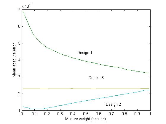
Figure 2: Dependence of the relative median absolute error from the mixture weight $\epsilon$.

To illustrate the dependence of the estimation error on the choice of the mixture weight $\epsilon$ for the three considered designs. We fix the number of agents $n=32$ and the sample size $N=1000$ and vary mixture probability $\epsilon$ between 0 an 1, exclusive. In Figure 2 we demonstrate the dependence of the median absolute error computed as the ratio of the median absolute error to estimated revenue. The figure demonstrates that for Designs 1 and 3, error decreases or remains constant as $\epsilon$ increases. This is consistent with our theoretical bound. On the other hand, for Design 2, after a small initial decrease, the error surprisingly increases with $\epsilon$. This increase is not directly captured by our theoretical bound. Intuitively, the auction A in Design 2 is much better for inferring the revenue of B than B itself, because the bid distribution it generates has high density on its entire range.

5 Applications to A/B testing

We now discuss applications of the inference approach we developed in Section 3.

5.1 Estimating revenues of novel mechanisms

Recall the setting of an ideal A/B test: an auction house running auction $A$ and wanting to determine the revenue of a novel mechanism $B$ mixes in the auction $B$ with some probability $\epsilon>0$. Suppose that in doing so, the auction house obtains $\epsilon N$ bids in response to the auction $B$ out of a total of $N$ bids, the revenue of $B$ can be estimated within an error bound of

$$\Theta\left(\frac{1}{\sqrt{\epsilon}}\right)\frac{\sup_{q}\{x_{B}^{\prime}(q)\}}{\sqrt{N}}.$$ (9)

In practice, however, instead of obtaining bids in response to $B$ alone, the seller obtains bids in response to the aggregate mechanism $C=(1-\epsilon)A+\epsilon B$. We can then use (5) to estimate the revenue of $B$. As a consequence of Theorem 3.4, and noting that for positions auctions with $n$ positions, $x_{C}^{\prime}(q)\leq n$ and $x_{B}^{\prime}(q)/x_{C}^{\prime}(q)\leq 1/\epsilon$ for all quantiles $q$, we obtain the following error bound.

Corollary 5.1.

The revenue of a rank based mechanism $B$ can be estimated from $N$ bids of a rank-based mechanism $C=(1-\epsilon)A+\epsilon B$ with absolute error bounded by

$$O(1)\sqrt{n\log n}\log(n/\epsilon)\,\,\frac{\sup_{q}\{x_{B}^{\prime}(q)\}}{\sqrt{N}}.$$ (10)

Relative to the ideal situation described above, our error bound has a better dependence on $\epsilon$ and a worse dependence on $n$. Note that when $\epsilon$ is very small, our error bound (10) may be smaller than the ideal bound in (9). This is not surprising: the ideal bound ignores information that we can learn about the revenue of $B$ from the $(1-\epsilon)N$ bids obtained when $B$ is not run.

When $B$ is a multi-unit auction, we obtain a better error bound using Theorem 3.3 which is closer to the ideal bound in (9).

Corollary 5.2.

The revenue of the highest-$k$-bids-win mechanism $B$ can be estimated from $N$ bids of a rank-based mechanism $C=(1-\epsilon)A+\epsilon B$ with absolute error bounded by

$$40\log(n/\epsilon)\,\,\frac{\sup_{q}\{x_{B}^{\prime}(q)\}}{\sqrt{N}}.$$ (11)

5.2 Universal B test

We now consider the problem of estimating all of the multi-unit revenues $P_{k}$ simultaneously from the bids of a single auction. What properties should the auction C have in order to enable this? The following definition formalizes this notion.

Definition 5.3.

An auction B is a universal B test if for any rank-based auction A, any $\epsilon>0$, and auction C defined by $x_{C}=(1-\epsilon)x_{A}+\epsilon x_{B}$; all of the multi-unit revenues $P_{1},\ldots,P_{n}$ can be estimated from bids of C with the dependence of the absolute error on $\epsilon$ bounded by $O(\log(1/\epsilon))$.

In Chawla et al. (6) we showed that it suffices to mix the $k$-unit auction for every $k$ into C with some small probability. In other words, the position auction B with position weights $w_{k}=1-k/n$ is a universal B test. We will now prove that in fact we can get similar results by mixing in just a few of the multi-unit auctions. In particular, in order to estimate $P_{k}$ accurately, it suffices to mix in a multi-unit auction with no more than $k$ units, and another one with no less than $k$ units. This gives us a more efficient universal B test for simultaneously inferring all of the multi-unit revenues (see Corollary 5.6).

Lemma 5.4.

The revenue of the highest-$k$-bids-win mechanism B can be estimated from $N$ bids of a rank-based all-pay auction C $=$ $(1-2\epsilon)$A $+\epsilon$B${}_{1}+\epsilon$B₂ where A is an arbitrary rank-based auction, and B₁ and B₂ are the highest-$k_{1}$-bids-win and highest-$k_{2}$-bids-win auctions respectively, with $k_{1}\leq k\leq k_{2}$. The absolute error of the estimate is bounded by

$$40(n+\log(1/\epsilon))\,\,\frac{\sup_{q}\{x_{k}^{\prime}(q)\}}{\sqrt{N}}.$$

Proof 5.5.

We begin by noting that for any $j$ and $k$ with $k\leq j$,

$$\frac{x^{\prime}_{k}(q)}{x^{\prime}_{j}(q)}=\frac{{j-1\choose k-1}}{{{n-1-k}\choose{n-1-j}}}\left(\frac{q}{1-q}\right)^{j-k}.$$

When $k\leq j$ and $q\geq 1/2$, this ratio is less than $2^{n}$. Likewise, we can show that when $k\geq j$ and $q\leq 1/2$, the ratio $\frac{x^{\prime}_{k}(q)}{x^{\prime}_{j}(q)}$ is less than $2^{n}$. Therefore, for any $q$, and C $=(1-2\epsilon)$A $+\epsilon$B${}_{1}+\epsilon$B₂ where B₁ and B₂ are the highest-$k_{1}$-bids-win and highest-$k_{2}$-bids-win auctions respectively, with $k_{1}\leq k\leq k_{2}$, we have

$$\frac{x^{\prime}_{k}(q)}{x^{\prime}_{C}(q)}\leq\frac{1}{\epsilon}2^{n}.$$

Next we note that $\sup_{q}x^{\prime}_{C}(q)\leq n$, and therefore, $\sup_{q:x_{k}^{\prime}(q)\geq 1}\frac{x_{C}^{\prime}(q)}{x_{k}^{\prime}(q)}\leq n$. Putting these quantities together with Theorem 3.3, we get that the absolute error in estimating $P_{k}$ from bids drawn from C is at most

$$\text{\bf E}_{\hat{b}}\!\left[|\hat{P_{k}}-P_{k}|\right] \leq\frac{40}{\sqrt{N}}\,\,\sup_{q}\{x_{k}^{\prime}(q)\}\,\,\left(n+\log 1/\epsilon\right).$$

Corollary 5.6.

Let B be the position auction with position weights $w_{1}=1$, $w_{k}=1/2$ for $1<k<n-1$, and $w_{n}=0$. Then $N$ bids from a mechanism C with $x_{C}=(1-\epsilon)x_{A}+\epsilon x_{B}$, where A is an arbitrary rank-based auction, can be used to simultaneously estimate all of the multi-unit revenues, and consequently all position auction revenues with absolute error bounded by

$$\frac{40n(n+\log(1/\epsilon))}{\sqrt{N}}.$$

5.3 Comparing revenues

We have considered the case where the empirical task was to recover the revenues for one mechanism ($y$) using the sample of bids responding to another mechanism ($x$). In many practical situations the empirical task is simply the verification of whether the revenue from a given mechanism is higher than the revenue from another mechanism. Or, equivalently, the task could be to verify whether one mechanism provides revenue which is a certain percentage above that of another mechanism. We now demonstrate that this is a much easier empirical task in terms of accuracy than the task of inferring the revenue.

Suppose that we want to compare the revenues of mechanisms $B_{1}$ and $B_{2}$ by mixing them in to an incumbent mechanism $A$, and running the composite mechanism $C=\epsilon B_{1}+\epsilon B_{2}+(1-2\epsilon)A$. Specifically, we would like to determine whether $P_{B_{1}}>\alpha P_{B_{2}}$ for some $\alpha>0$. Consider a binary classifier $\widehat{\gamma}$ which is equal to $1$ when $P_{B_{1}}>\alpha P_{B_{2}}$ and $0$ otherwise. Let $\gamma={\bf 1}\{P_{B_{1}}-\alpha\,P_{B_{2}}>0\}$ be the corresponding “ideal” classifier for the case where the distribution of bids from mechanism $C$ is known precisely. To evaluate the accuracy of the classifier, we need to evaluate the probability $\Pr(\widehat{\gamma}=1|\gamma=0)$, and likewise, $\Pr(\widehat{\gamma}=0|\gamma=1)$. The classifier will give the wrong output if the sampling noise in estimating $\hat{P}_{B_{1}}-\alpha\,\hat{P}_{B_{2}}$ is greater than $|P_{B_{1}}-\alpha\,P_{B_{2}}|$.

Our main result of this section says that keeping $\alpha$, the difference $|P_{B_{1}}-\alpha\,P_{B_{2}}|$, and the number of positions $n$ constant, the probability of incorrect output decreases exponentially with the number of bids $N$. See Appendix D for a proof.

Theorem 5.7.

Suppose that $N$ bids from a mechanism $C=\epsilon B_{1}+\epsilon B_{2}+(1-2\epsilon)A$ for arbitrary rank-based mechanisms $B_{1}$, $B_{2}$, and $A$, are used to estimate the classifier $\gamma={\bf 1}\{P_{B_{1}}-\alpha\,P_{B_{2}}>0\}$ that establishes whether the revenue of mechanism $B_{1}$ exceeds $\alpha$ times the revenue of mechanism $B_{2}$. Then the error rate of the binary classifier is bounded from above by

$$\exp\left(-O\left(\frac{Na^{2}}{\alpha^{2}n^{3}\log(n/\epsilon)}\right)\right),$$

where $a=|P_{B_{1}}-\alpha\,P_{B_{2}}|$. In other words, once the number of samples is polynomially large in $n$, the error rate decreases exponentially with the number of samples.

We obtain a similar error bound when our goal is to estimate which of $r$ different novel mechanisms obtains the most revenue, for any $r>1$:

Corollary 5.8.

Suppose that our goal is to determine which of $r$ position auctions, $B_{1},B_{2},\cdots,B_{r}$, obtains the most revenue while running incumbent mechanism $A$, by running each of the novel mechanisms with probability $\epsilon/r$. Then the error probability of the corresponding classifier constructed using $N$ bids from composite mechanism $C=\sum_{i=1}^{r}\epsilon/rB_{i}+(1-\epsilon)A$ is bounded from above by

$$r\exp\left(-O\left(\frac{Na^{2}}{n^{3}\log(rn/\epsilon)}\right)\right),$$

where $a$ is the absolute difference between the revenue obtained by the best two of the $r$ mechanisms.

Appendix A Inference for Auctions

The distribution of values, which is unobserved, can be inferred from the distribution of bids, which is observed. Once the value distribution is inferred, other properties of the value distribution such as its corresponding revenue curve, which is fundamental for optimizing revenue, can be obtained. In this section we describe the basic premise of the inference assuming that the distribution of bids known exactly.

The key idea behind the inference of the value distribution from the bid distribution is that the strategy which maps values to bids is a best response, by equation (1), to the distribution of bids. As the distribution of bids is observed, and given suitable continuity assumptions, this best response function can be inverted.

The value distribution can be equivalently specified by distribution function $F(\cdot)$ or value function $v(\cdot)$; the bid distribution can similarly be specified by the bid function $b(\cdot)$. For rank-based auctions (as considered by this paper) the allocation rule $x(\cdot)$ in quantile space is known precisely (i.e. it does not depend on the value function $v(\cdot)$). Assume these functions are monotone, continuously differentiable, and invertible.

Inference for first-price auctions

Consider a first-price rank-based auction with a symmetric bid function $b(q)$ and allocation rule $x(q)$ in BNE. To invert the bid function we solve for the bid that the agent with any quantile would make. Continuity of this bid function implies that its inverse is well defined. Applying this inverse to the bid distribution gives the value distribution.

The utility of an agent with quantile $q$ as a function of his bid $z$ is

$$u(q,z) =(v(q)-z)\,x(b^{-1}(z)).$$ (12)

Differentiating with respect to $$z$$ we get:

$$\tfrac{d}{dz}u(q,z) =-x(b^{-1}(z))+\big{(}v(q)-z\big{)}\,x^{\prime}(b^{-1}(z))\,\tfrac{d}{dz}b^{-1}(z).$$

Here $$x^{\prime} x q b(\cdot) \tfrac{d}{dz}u(q,z) 0 z=b(q)$$ is the derivative of with respect to the quantile . Because is in BNE, the derivative is at . Rarranging, we obtain:

$$v(q) =b(q)+\tfrac{x(q)\,b^{\prime}(q)}{x^{\prime}(q)}$$

Inference for all-pay auctions

We repeat the calculation above for rank-based all-pay auctions; the starting equation (12) is replaced with the analogous equation for all-pay auctions:

$$u(q,z) =v(q)\,x(b^{-1}(z))-z.$$ (13)

Differentiating with respect to $$z$$ we obtain:

$$\tfrac{d}{dz}u(q,z) =v(q)\,x^{\prime}(b^{-1}(z))\,\frac{d}{dz}b^{-1}(z)-1,$$

Again the first-order condition of BNE implies that this expression is zero at $$z=b(q)$$; therefore,

$$v(q) =\tfrac{b^{\prime}(q)}{x^{\prime}(q)}.$$

Known and observed quantities

Recall that the functions $x(q)$ and $x^{\prime}(q)$ are known precisely: these are determined by the rank-based auction definition. The functions $b(q)$ and $b^{\prime}(q)$ are observed. The calculations above hold in the limit as the number of samples from the bid distribution goes to infinity, at which point these obserations are precise.

Appendix B Inference for social welfare

We now consider the problem of estimating the social welfare of a rank-based auction using bids from another rank-based all-pay auction. Consider a rank-based auction with induced position weights $\boldsymbol{w}$. By definition, the expected per-agent social welfare obtained by this auction is as below, where $V_{k}$ is the expected value of the $k$th highest value agent, or the $k$th order statistic of the value distribution.

$$S_{\boldsymbol{w}}=\frac{1}{n}\sum_{k=1}^{n}w_{k}V_{k}$$

We note that the value order statistics, $V_{k}$, are closely related to the expected revenues of the multi-unit auctions. The $k$-unit second-price auction serves the top $k$ agents with probability $1$, and charges each agent the $k+1$th highest value. Its expected revenue is therefore $nP_{k}=kV_{k+1}$. We therefore obtain:

$$S_{\boldsymbol{w}}=w_{1}\frac{V_{1}}{n}+\sum_{k=1}^{n-1}w_{k+1}\,\frac{P_{k}}{k}$$

The methodology developed in the previous sections can be used to estimate the $P_{k}$’s in the above expression. The first order statistic of the values, $V_{1}$, cannot be directly estimated in this manner. Notate the expected value of an agent as

$$\mathcal{V}=\text{\bf E}_{q}\!\left[v(q)\right]=\frac{1}{n}\sum_{k=1}^{n}V_{k}$$

where $\mathcal{V}$ is the expected value of any one agent. Therefore, we can calculate the social welfare of the position auction with weights $\boldsymbol{w}$ as

$$S_{\boldsymbol{w}}=w_{1}\mathcal{V}-\sum_{k=2}^{n}(w_{1}-w_{k})\frac{V_{k}}{n}=w_{1}\mathcal{V}-\sum_{k=1}^{n-1}(w_{1}-w_{k+1})\,\frac{P_{k}}{k}$$ (14)

We now argue that $\mathcal{V}$ can be estimated at a good rate from the bids of another rank-based all-pay auction. Let $x$ denote the allocation rule of the auction that we run, and $b$ denote the bid distribution in BNE of this auction. Then we note that

$$\mathcal{V}=\text{\bf E}_{q}\!\left[v(q)\right]=\text{\bf E}_{q}\!\left[\frac{b^{\prime}(q)}{x^{\prime}(q)}\right]=\text{\bf E}_{q}\!\left[-\bar{Z}^{\prime}(q)b(q)\right]$$

where $\bar{Z}(q)=1/x^{\prime}(q)$. We might now try to directly apply Theorem 3.3 to bound the error in our estimate of $\mathcal{V}$. This does not work, as Lemma D.1 fails to hold for $\bar{Z}$. Instead, we can follow the argument in the proof of Theorem 3.4 and obtain the following lemma:

Lemma B.1.

The expected absolute error in estimating the expected value $\mathcal{V}$ using $N$ samples from the bid distribution for an all-pay position auction with allocation rule $x$ is bounded as below; Here $n$ is the number of positions in the position auction.

$$\text{\bf E}_{\hat{b}}\!\left[|\hat{\mathcal{V}}-\mathcal{V}|\right] \leq\tfrac{40}{\sqrt{N}}\sqrt{n\log n}\,\,\log\max\left\{\sup\nolimits_{q}x^{\prime}(q),\sup\nolimits_{q}\tfrac{1}{x^{\prime}(q)}\right\}$$

$$\quad+\tfrac{O(1)}{N}\sup\nolimits_{q}\{x^{\prime}(q)\}\,\,\sup\nolimits_{q}\left\{\tfrac{1}{x^{\prime}(q)}\right\}$$

As an example application of Lemma B.1, we adapt Corollary 5.6 to bound the error of from estimating the social welfare of any position auction that is mixed with the universal B test mechanism of Section 5.2. Other revenue estimation results can be similarly adapted to estimate social welfare.

Theorem B.2.

Let B be the position auction with position weights $w_{1}=1$, $w_{k}=1/2$ for $1<k<n-1$, and $w_{n}=0$. Then $N$ bids from a mechanism C with $x_{C}=(1-\epsilon)x_{A}+\epsilon x_{B}$, where A is an arbitrary rank-based auction, can be used to simultaneously estimate the per-agent social welfare of any rank-based mechanism with absolute error bounded by

$$\frac{40n\log n(n+\log(1/\epsilon))}{\sqrt{N}}+\frac{40\sqrt{n\log n}\log(n/\epsilon)}{\sqrt{N}}+O\left(\frac{n}{\epsilon N}\right)=O\left(\frac{n\log n(n+\log(1/\epsilon))}{\sqrt{N}}\right)+O\left(\frac{n}{\epsilon N}\right).$$

The theorem follows by combining Lemma B.1 with equation (14) and Corollary 5.6. In the statement of the theorem the error term corresponding to the $P_{k}$’s has an extra factor of $\log n$ (relative to the statement of Corollary 5.6) because the total weight of the multipliers for the terms in equation (14) can be as large as $\log n$.

Appendix C Inference methodology and error bounds for first-price auctions

While most of our analysis so far has focused on the case of all-pay auctions, our methodology and results extend as-is to first-price auctions as well. Here we sketch the differences between the two cases.

Recall that in a first-price auction, we can obtain the value distribution from the bid distribution as follows: $v(q)=b(q)+x(q)b^{\prime}(q)/x^{\prime}(q)$. Substituting this into the expression for $P_{y}$ we get:

$$P_{y}=\text{\bf E}_{q}\!\left[(1-q)y^{\prime}(q)b(q)+\frac{(1-q)y^{\prime}(q)x(q)b^{\prime}(q)}{x^{\prime}(q)}\right]=\text{\bf E}_{q}\!\left[(1-q)y^{\prime}(q)b(q)+Z_{y}(q)x(q)b^{\prime}(q)\right]$$

where, as before, $Z_{y}(q)=\frac{(1-q)y^{\prime}(q)}{x^{\prime}(q)}$.

Integrating the second expression by parts, we get

$$\int_{0}^{1}Z_{y}(q)x(q)b^{\prime}(q)\,dq = Z_{y}(q)x(q)b(q)|_{0}^{1}-\int_{0}^{1}(Z^{\prime}_{y}(q)x(q)+Z_{y}(q)x^{\prime}(q))b(q)\,dq$$

$$= -\int_{0}^{1}Z^{\prime}_{y}(q)x(q)b(q)\,dq-\int_{0}^{1}(1-q)y^{\prime}(q)b(q)\,dq$$

When we put this back in the expression for $P_{y}$ two of the terms cancel, and we get the following lemma.

Lemma C.1.

The per-agent revenue of an auction with allocation rule $y$ can be written as a linear combination of the bids in a first-pay auction:

$$P_{y}=\text{\bf E}_{q}\!\left[-x(q)Z^{\prime}_{y}(q)b(q)\right]$$

where $Z_{y}(q)=(1-q)\frac{y^{\prime}(q)}{x^{\prime}(q)}$ and $x(q)$ are known precisely.

As in the case of the all-pay auction format, we can write the error in $P_{y}$ as:

$$|\hat{P}_{y}-P_{y}| = \text{\bf E}_{q}\!\left[\left|-x(q)Z^{\prime}_{y}(q)(\widehat{b}(q)-b(q))\right|\right]$$

$$\leq E\left[\frac{\left(\log(1+Z_{y}(q))\right)^{\alpha}}{Z_{y}(q)}|Z^{\prime}_{y}(q)|\right]\sup\limits_{q}\left|x(q)\frac{Z_{y}(q)}{\left(\log(1+Z_{y}(q))\right)^{\alpha}}(\hat{b}(q)-b(q))\right|$$

With an appropriate choice of $\alpha$ we obtain the following theorem.

Theorem C.2.

The expected absolute error in estimating the revenue of a position auction with allocation rule $y$ using $N$ samples from the bid distribution for a first-pay position auction with allocation rule $x$ is bounded as below; Here $n$ is the number of positions in the two position auctions.

$$\text{\bf E}_{\hat{b}}\!\left[|\hat{P_{y}}-P_{y}|\right] \leq\frac{40}{\sqrt{N}}\sqrt{n\log n}\,\,\sup_{q}\{y^{\prime}(q)\}\,\,\log\max\left\{\sup_{q:y^{\prime}(q)\geq 1}\frac{x^{\prime}(q)}{y^{\prime}(q)},\sup_{q}\frac{y^{\prime}(q)}{x^{\prime}(q)}\right\}$$

$$+\frac{O(1)}{N}\sup_{q}\{x^{\prime}(q)\}\,\,\sup_{q}\left\{\frac{y^{\prime}(q)}{x^{\prime}(q)}\right\}.$$

When $y$ is the highest-$k$-bids-win allocation rule, the error improves to:

$$\text{\bf E}_{\hat{b}}\!\left[|\hat{P_{k}}-P_{k}|\right] \leq\frac{40}{\sqrt{N}}\,\,\sup_{q}\{x_{k}^{\prime}(q)\}\,\,\log\max\left\{\sup_{q:x_{k}^{\prime}(q)\geq 1}\frac{x^{\prime}(q)}{x_{k}^{\prime}(q)},\sup_{q}\frac{x_{k}^{\prime}(q)}{x^{\prime}(q)}\right\}.$$

Because the error bounds in Theorem C.2 are identical to those in Theorems 3.3 and 3.4, Lemma 5.4, Corollaries 5.1, 5.2, 5.6, and Theorems 5.7 and B.2 continue to hold when bids are drawn from a first-price auction.

Appendix D Missing proofs

Fact 1.

The maximum slope of the allocation rule $x$ of any $n$-agent position auction is bounded by $n$: $\sup_{q}x^{\prime}(q)\leq n$. The maximum slope of the allocation rule $x_{k}$ for the $n$-agent highest-$k$-bids-win auction is bounded by

$$\sup_{q}x_{k}^{\prime}(q)\in\left[\frac{1}{\sqrt{2\pi}},\frac{1}{\sqrt{\pi}}\right]\frac{n-1}{\sqrt{\min\{k-1,n-k\}}}=\Theta\left(\frac{n}{\sqrt{\min\{k,n-k\}}}\right).$$

Proof of Theorem 3.3. We will make use of the following lemma from Chawla et al. (6).

Lemma D.1 (Chawla et al. (6) ).

Let $x_{k}$ denote the allocation function of the $k$-highest-bids-win auction and $x$ be any convex combination over the allocation functions of the multi-unit auctions. Then the function $Z_{k}(q)=(1-q)\frac{x_{k}^{\prime}(q)}{x^{\prime}(q)}$ achieves a single local maximum for $q\in[0,1]$.

Recall that for $\alpha>0$ we can write

$$|\hat{P}_{k}-P_{k}|\leq E\left[\frac{\left(\log(1+Z_{k}(q))\right)^{\alpha}}{Z_{k}(q)}|Z^{\prime}_{k}(q)|\right]\sup\limits_{q}\left|\frac{Z_{k}(q)}{\left(\log(1+Z_{k}(q))\right)^{\alpha}}(\hat{b}(q)-b(q))\right|$$

We start by considering the first term. Lemma D.1 shows that $Z^{\prime}_{k}(\cdot)$ changes sign only once. Consider the region where the sign of $Z^{\prime}_{k}(\cdot)$ is constant and make the change of variable $t=Z_{k}(q)$. Recall that $Z_{k}^{*}=\sup_{q}Z_{k}(q)$ and we note that $\inf_{q}Z_{k}(q)\geq 0$. Then we can evaluate the first term as

$$E\left[\frac{\left(\log(1+Z_{k}(q))\right)^{\alpha}}{Z_{k}(q)}|Z^{\prime}_{k}(q)|\right]\leq 2\int^{Z_{k}^{*}}_{0}\frac{(\log\,(1+t))^{\alpha}}{t}\,dt$$

Note that for any $t>0$, $\log(1+t)\leq t$. Thus,

$$\int^{\delta}_{0}\frac{(\log\,(1+t))^{\alpha}}{t}\,dt<\frac{\delta^{\alpha}}{\alpha}$$

Now split the integral into two pieces as

$$\int^{Z_{k}^{*}}_{0}\frac{(\log\,(1+t))^{\alpha}}{t}\,dt=\int^{1}_{0}\frac{(\log\,(1+t))^{\alpha}}{t}\,dt+\int^{Z_{k}^{*}}_{1}\frac{(\log\,(1+t))^{\alpha}}{t}\,dt$$

We just proved that the first piece is at most $1/\alpha$. Now we upper bound the second piece and consider the integrand at $t\geq 1$. First, note that

$$(\log\,(1+t))^{\alpha}=\left(\log\,t+\log(1+\frac{1}{t})\right)^{\alpha}\leq\left(\log\,t+\frac{1}{t}\right)^{\alpha}\leq(\log\,t+1)^{\alpha}.$$

Thus, the integral behaves as

$$\int^{Z_{k}^{*}}_{1}\frac{(\log\,(1+t))^{\alpha}}{t}\,dt\leq\int^{Z_{k}^{*}}_{1}\frac{(\log\,(t)+1)^{\alpha}}{t}\,dt=\frac{1}{1+\alpha}(\log\,Z_{k}^{*}+1)^{1+\alpha}.$$

Thus, we just showed that

$$E\left[\frac{\left(\log(1+Z_{k}(q))\right)^{\alpha}}{Z_{k}(q)}|Z^{\prime}_{k}(q)|\right]\leq\frac{2}{\alpha}+\frac{2}{1+\alpha}(\log\,Z_{k}^{*}+1)^{1+\alpha},$$

which is at most $2(1+e)/\alpha$ for $\alpha<1/\log\,Z_{k}^{*}$.

Now consider the term

$$\sup\limits_{q}\left|\frac{Z_{k}(q)}{\left(\log(1+Z_{k}(q))\right)^{\alpha}}(\hat{b}(q)-b(q))\right|$$

Note that $\log(1+t)\geq\min\{1,t\}/2$. So the first term can be bounded from above as

$$\frac{Z_{k}(q)}{\left(\log(1+Z_{k}(q))\right)^{\alpha}}\leq 2^{\alpha}\max\left\{Z_{k}(q),\,(Z_{k}(q))^{1-\alpha}\right\}$$

The second term behaves as

$$(\hat{b}(q)-b(q))=-x^{\prime}(q)v(q)(\hat{G}(b(q))-G(b(q)))$$

where $G$ and $\hat{G}$ are the real and empirical bid distributions, respectively. We recall that $\text{\bf E}\!\left[\sup_{q}\left|\hat{G}(b(q))-G(b(q))\right|\right]\leq\frac{1}{2\sqrt{N}}$. Thus

$$\text{\bf E}\!\left[\sup\limits_{q}\left|\frac{Z_{k}(q)}{\left(\log(1+Z_{k}(q))\right)^{\alpha}}(\hat{b}(q)-b(q))\right|\right] \leq 2^{\alpha}\sup_{q}\left(\max\left\{x^{\prime}_{k}(q),\,(x^{\prime}_{k}(q))^{1-\alpha}(x^{\prime}(q))^{\alpha}\right\}\right)\frac{1}{2\sqrt{N}}$$

$$\leq 2^{\alpha}\sup_{q}\left(x^{\prime}_{k}(q)\right)\left(\underbrace{\max\left(1,\sup_{q:x^{\prime}_{k}(q)\geq 1}\frac{x^{\prime}(q)}{x^{\prime}_{k}(q)}\right)}_{=:\,A}\right)^{\alpha}\frac{1}{2\sqrt{N}}$$

Now we combine the two evaluations together and pick $\alpha=\min\{1/\log A,1/\log Z_{k}^{*}\}$, with $A$ defined as above, to obtain

$$\text{\bf E}\!\left[|\hat{P}_{k}-P_{k}|\right] \leq\frac{2(1+e)}{\alpha}2^{\alpha}A^{\alpha}\frac{1}{2\sqrt{N}}\sup_{q}\left(x^{\prime}_{k}(q)\right)$$

$$\leq\frac{20}{\sqrt{N}}\,\,\sup_{q}\{x_{k}^{\prime}(q)\}\,\,\max\left\{\log A,\log\sup_{q}\left\{\frac{x_{k}^{\prime}(q)}{x^{\prime}(q)}\right\}\right\}$$

∎

Proof of Lemma 3.5. We can write the function $\tilde{b}(i/N)$ as

$$\tilde{b}\left(\frac{i}{N}\right) =\frac{N!}{(i-1)!(N-i)!}\int G(t)^{i-1}(1-G(t))^{N-i}g(t)t\,dt$$

$$=\frac{N!}{(i-1)!(N-i)!}\int t^{i-1}(1-t)^{N-i}b(t)\,dt$$

Note that

$$\frac{N!}{(i-1)!(N-i)!}t^{i-1}(1-t)^{N-i}$$

is the density of the beta-distribution with parameters $\alpha=i$ and $\beta=N-i+1$. Denote this density $f(t;\alpha,\beta)$. Then we can write

$$\tilde{b}\left(\frac{i}{N}\right)=\int^{1}_{0}b(t)f(t;\alpha,\beta)\,dt.$$

Now let $q\in[i/N,\,(i+1)/N]$, and consider an expansion of $b(t)$ at $q$ such that

$$b(t)=b(q)+b^{\prime}(q)(t-q)+O((t-q)^{2})$$

Now we substitute this expansion into the formula for $\tilde{b}(\cdot)$ above to get

$$\tilde{b}\left(\frac{i}{N}\right)=b(q)+b^{\prime}(q)\int^{1}_{0}(t-q)f(t;\alpha,\beta)\,dt+O(\int^{1}_{0}(t-q)^{2}f(t;\alpha,\beta)\,dt)$$

The mean of the beta distribution is $\alpha/(\alpha+\beta)$ and the variance is $\alpha\beta/((\alpha+\beta)^{2}(\alpha+\beta+1))$. This means that

$$\tilde{b}\left(\frac{i}{N}\right)-b(q)=b^{\prime}(q)\left(\frac{i}{N+1}-q\right)+O\left(\frac{1}{N^{2}}\right).$$

Thus

$$\sup_{q\in[i/N,(i+1)/N]}\left|\tilde{b}\left(\frac{i}{N}\right)-b(q)\right|\leq\sup_{q}b^{\prime}(q)\frac{2}{N}+O\left(\frac{1}{N^{2}}\right).$$

Therefore, the expectation $\left|\hat{P}_{y}-\text{\bf E}\!\left[\hat{P}_{y}\right]\right|$ is at most $O(1)/N\,\sup_{q}\{x^{\prime}(q)\}\,\sup_{q}Z_{y}(q)$. ∎

Proof of Lemma 3.6. Fix $I$ and $\ell$, and note that the function $\tilde{b}$ is fixed (that is, it does not depend on the empirical bid sample). Then, the sum $\mathbf{T}_{i_{\ell},i_{\ell+1}}$ depends only on the empirical bid values $\widehat{b}(q)$ for quantiles in the interval $[i_{\ell}/N,i_{\ell+1}/N)$. By the definition of $I$, we know that the smallest $i_{\ell}$ bids in the sample are all smaller than $\tilde{b}((i_{\ell}-1)/N)\leq\tilde{b}(i_{\ell}/N)$, and the largest $N-i_{\ell+1}$ bids in the sample are all larger than $\tilde{b}(i_{\ell+1}/N)\geq\tilde{b}((i_{\ell+1}-1)/N)$. On the other hand, the empirical bids $\widehat{b}(q)$ for $q\in[i_{\ell}/N,i_{\ell+1}/N)$ lie within $[\tilde{b}(i_{\ell}/N),\tilde{b}((i_{\ell+1}-1)/N)]$. Therefore, conditioned on $i_{\ell}$ and $i_{\ell+1}$, the latter set of empirical bids is independent of the former set of empirical bids. ∎

Proof of Lemma 3.7 and Theorem 3.4. We will use Chernoff-Hoeffding bounds to bound the expectation of $\mathbf{T}_{0,N}$ over the bid sample, conditioned on $I$ and $\Delta=\sup_{q\in[0,1]}|\hat{G}(b(q))-G(b(q))|$. We first note that $\mathbf{T}_{0,N}$ has mean zero because for any integer $i\in[0,N]$, $\text{\bf E}_{\text{samples}}\!\left[\widehat{b}(i/N)\right]=\tilde{b}(i/N)$.

Next we note that the $\mathbf{T}_{i,j}$’s are bounded random variables. Specifically, let $Q$ be an interval of quantiles over which the difference $\widehat{b}(q)-\tilde{b}(q)$ does not change sign. Then, following the proof of Theorem 3.3, we can bound

$$|\mathbf{T}_{Q}| =\left|\int_{Q}Z^{\prime}_{y}(q)(\widehat{b}(q)-\tilde{b}(q))\,\text{d}q\right|$$

$$\leq 20\Delta\underbrace{\,\,\sup_{q}\{y^{\prime}(q)\}\,\,\log\max\left\{\sup_{q:y^{\prime}(q)\geq 1}\frac{x^{\prime}(q)}{y^{\prime}(q)},\sup_{q}\frac{y^{\prime}(q)}{x^{\prime}(q)}\right\}}_{=:\,S}.$$

Likewise, over an interval $Q$ where $Z^{\prime}_{y}$ does not change sign, we again get $|\mathbf{T}_{Q}|\leq 20\Delta S$ with $S$ defined as above. Moreover, for an interval $Q$ over which $Z^{\prime}_{y}$ changes sign at most $t$ times, we have

$$\int_{Q}|Z^{\prime}_{y}(q)(\widehat{b}(q)-\tilde{b}(q))|\,\text{d}q\leq t\cdot 20\Delta S.$$

Finally, noting that $Z_{y}$ is a weighted sum over the $n$ functions $Z_{k}$ defined for the $k$-unit auctions, and that by Lemma D.1 each $Z_{k}$ has a unique maximum, we note that $Z^{\prime}_{y}$ changes sign at most $2n$ times.

We now apply Chernoff-Hoeffding bounds to bound the probability that the sum $\sum_{\ell=0}^{\ell=k-1}\mathbf{T}_{i_{\ell},i_{\ell+1}}$ exceeds some constant $a$. With $\tau_{\ell}$ denoting the upper bound on $|\mathbf{T}_{i_{\ell},i_{\ell+1}}|$, this probability is at most

$$\text{exp}\left(-\frac{a^{2}}{\sum_{\ell}\tau_{\ell}^{2}}\right).$$

By our observations above, for all $\ell$, $\tau_{\ell}\leq 40\Delta S$, and $\sum_{\ell}\tau_{\ell}\leq\int_{0}^{1}|Z^{\prime}_{y}(q)(\widehat{b}(q)-\tilde{b}(q))|\,\text{d}q\leq 40n\Delta S$. Therefore, $\sum_{\ell}\tau_{\ell}^{2}\leq n(40\Delta S)^{2}$. We can now choose $a=\sqrt{n\log n}\,40\Delta S$ to make the above probability at most $1/n$.

Putting everything together, we get that conditioned on $I$ and $\Delta$, the expected value of $|\mathbf{T}_{0,N}|$ over the bid sample is at most $a+1/n\cdot 40n\Delta S=O(1)\sqrt{n\log n}\Delta S$. Since this bound is independent of $I$, the same bound holds when we remove the conditioning on $I$. The theorem now follows by plugging in the expected value of $\Delta$ from Lemma 2.2. ∎

Proof of Theorem 5.7. We need to bound the probability that the error in estimating $\hat{P}_{B_{1}}-\alpha\hat{P}_{B_{2}}$ is greater than $|P_{B_{1}}-\alpha\,P_{B_{2}}|$. This error can in turn be decomposed into the error in estimating $P_{B_{1}}$ and that in estimating $P_{B_{2}}$. Denote $a=|P_{B_{1}}-\alpha\,P_{B_{2}}|>0$. Then,

$$\Pr\left(|(\widehat{P}_{B_{1}}-\alpha\,\widehat{P}_{B_{2}})-(P_{B_{1}}-\alpha\,P_{B_{2}})|>a\right)\leq\Pr\left(|\widehat{P}_{B_{1}}-P_{B_{1}}|>a/2\right)+\Pr\left(|\widehat{P}_{B_{2}}-P_{B_{2}}|>a/2\alpha\right).$$

Let $x$ denote the allocation rule of the mechanism $C$ that we are running, and let $b$ be the corresponding bid function. Now, recall that for

$$\Delta=\sup_{q}|\widehat{G}(b(q))-G(b(q))|,\,\,\,\text{and }\,\,S=\sup_{q}\{x_{B_{1}}^{\prime}(q)\}\log\max\left\{\sup_{q:x^{\prime}_{B_{1}}(q)\geq 1}\frac{x^{\prime}(q)}{x_{B_{1}}^{\prime}(q)},\sup_{q}\frac{x_{B_{1}}^{\prime}(q)}{x^{\prime}(q)}\right\},$$

Equation (8), Lemma 3.5, and Lemma 3.7 together imply that (conditional on $\Delta$)

$$\Pr\left(|\widehat{P}_{B_{1}}-P_{B_{1}}|>a/2\right)\leq 2\exp\left(-\frac{1}{n(40\,\Delta\,S)^{2}}\left(\frac{a}{2}-O\left(\frac{n}{\epsilon N}\right)\right)^{2}\right).$$

Now recall that $S<n\log(n/\epsilon)$, and $\Delta<\text{constant}/\sqrt{N}$ with high probability (Lemma 2.2). As a result, we establish that for $a=\omega(n/\epsilon N)$,

$$\Pr\left(|\widehat{P}_{B_{1}}-P_{B_{1}}|>a/2\right)\leq\exp\left(-O\left(\frac{Na^{2}}{n^{3}\log(n/\epsilon)}\right)\right).$$

Likewise,

$$\Pr\left(|\widehat{P}_{B_{2}}-P_{B_{2}}|>a/2\alpha\right)\leq\exp\left(-O\left(\frac{Na^{2}}{\alpha^{2}n^{3}\log(n/\epsilon)}\right)\right).$$

∎

References

- Athey and Haile (2007) Athey, S. and Haile, P. A. 2007. Nonparametric approaches to auctions. Handbook of econometrics 6, 3847–3965.
- Baliga and Vohra (2003) Baliga, S. and Vohra, R. 2003. Market research and market design. Advances in Theoretical Economics 3, 1.
- Blum and Hartline (2005) Blum, A. and Hartline, J. D. 2005. Near-optimal online auctions. In Proceedings of the sixteenth annual ACM-SIAM symposium on Discrete algorithms. Society for Industrial and Applied Mathematics, 1156–1163.
- Brown and Morgan (2009) Brown, J. and Morgan, J. 2009. How much is a dollar worth? tipping versus equilibrium coexistence on competing online auction sites. Journal of Political Economy 117, 4, 668–700.
- Cesa-Bianchi et al. (2015) Cesa-Bianchi, N., Gentile, C., and Mansour, Y. 2015. Regret minimization for reserve prices in second-price auctions. IEEE Transactions on Information Theory 61, 1, 549.
- Chawla et al. (2014) Chawla, S., Hartline, J., and Nekipelov, D. 2014. Mechanism design for data science. In Proceedings of the fifteenth ACM conference on Economics and computation. ACM, 711–712.
- Chawla and Hartline (2013) Chawla, S. and Hartline, J. D. 2013. Auctions with unique equilibria. In Proceedings of the Fourteenth ACM Conference on Electronic Commerce. EC ’13. ACM, New York, NY, USA, 181–196.
- Cheng and Parzen (1997) Cheng, C. and Parzen, E. 1997. Unified estimators of smooth quantile and quantile density functions. Journal of statistical planning and inference 59, 2, 291–307.
- Cole and Roughgarden (2014) Cole, R. and Roughgarden, T. 2014. The sample complexity of revenue maximization. In Proceedings of the 46th Annual ACM Symposium on Theory of Computing. ACM, 243–252.
- Csörgö (1983) Csörgö, M. 1983. Quantile processes with statistical applications. SIAM.
- Csorgo and Revesz (1978) Csorgo, M. and Revesz, P. 1978. Strong approximations of the quantile process. The Annals of Statistics, 882–894.
- Edelman et al. (2007) Edelman, B., Ostrovsky, M., and Schwarz, M. 2007. Internet advertising and the generalized second-price auction: Selling billions of dollars worth of keywords. The American Economic Review 97, 1, 242–259.
- Fu et al. (2014) Fu, H., Haghpanah, N., Hartline, J., and Kleinberg, R. 2014. Optimal auctions for correlated buyers with sampling. In Proceedings of the fifteenth ACM conference on Economics and computation. ACM, 23–36.
- Goldberg et al. (2006) Goldberg, A. V., Hartline, J. D., Karlin, A. R., Saks, M., and Wright, A. 2006. Competitive auctions. Games and Economic Behavior 55, 2, 242–269.
- Gomes and Sweeney (2009) Gomes, R. and Sweeney, K. 2009. Bayes-nash equilibria of the generalized second price auction. In Proceedings of the 10th ACM conference on Electronic commerce. ACM, 107–108.
- Guerre et al. (2000) Guerre, E., Perrigne, I., and Vuong, Q. 2000. Optimal nonparametric estimation of first-price auctions. Econometrica 68, 3, 525–574.
- Hartline (2013) Hartline, J. D. 2013. Bayesian mechanism design. Foundations and Trends in Theoretical Computer Science 8, 3, 143–263.
- Kleinberg and Leighton (2003) Kleinberg, R. and Leighton, T. 2003. The value of knowing a demand curve: Bounds on regret for online posted-price auctions. In Foundations of Computer Science, 2003. Proceedings. 44th Annual IEEE Symposium on. IEEE, 594–605.
- Myerson (1981) Myerson, R. 1981. Optimal auction design. Mathematics of Operations Research 6, 58–73.
- Ostrovsky and Schwarz (2011) Ostrovsky, M. and Schwarz, M. 2011. Reserve prices in internet advertising auctions: A field experiment. In Proceedings of the 12th ACM Conference on Electronic Commerce. EC ’11. ACM, New York, NY, USA, 59–60.
- Paarsch and Hong (2006) Paarsch, H. J. and Hong, H. 2006. An introduction to the structural econometrics of auction data. Vol. 1. The MIT Press.
- Reiley (2006) Reiley, D. H. 2006. Field experiments on the effects of reserve prices in auctions: more magic on the internet. The RAND Journal of Economics 37, 1, 195–211.
- Segal (2003) Segal, I. 2003. Optimal pricing mechanisms with unknown demand. The American economic review 93, 3, 509–529.
- Varian (2007) Varian, H. 2007. Position auctions. International Journal of Industrial Organization 25, 6, 1163–1178.