Optimal quantization for a probability measure on a nonuniform stretched Sierpiński triangle

Abstract.

Quantization for a Borel probability measure refers to the idea of estimating a given probability by a discrete probability with support containing a finite number of elements. In this paper, we have considered a Borel probability measure $P$ on $\mathbb{R}^{2}$, which has support a nonuniform stretched Sierpiński triangle generated by a set of three contractive similarity mappings on $\mathbb{R}^{2}$. For this probability measure, we investigate the optimal sets of $n$-means and the $n$th quantization errors for all positive integers $n$.

1. Introduction

Optimal quantization is a fundamental problem in signal processing, data compression, and information theory. We refer to [GG, GN, Z2] for surveys on the subject and comprehensive lists of references to the literature; see also [AW, GKL, GL1, Z1]. For mathematical treatment of quantization, one is referred to Graf-Luschgy’s book (see [GL1]). Recently, Pandey and Roychowdhury introduced the concepts of constrained quantization and conditional quantization (see [PR1, PR2, PR4]). A quantization without a constraint is known as an unconstrained quantization, which, traditionally in the literature, is known as quantization. After the introduction of constrained quantization and then conditional quantization, the quantization theory is now much more enriched with huge applications in our real world. For some follow up papers in the direction of constrained quantization and conditional quantization, one can see [BCDR, BCDRV, HNPR, PR3, PR5]). On unconstrained quantization, there is a number of papers written by many authors; for example, one can see [DFG, DR, GG, GL, GL1, GL2, GL3, GN, KNZ, P, P1, R1, R2, R3, Z1, Z2].

Definition 1.1.

Let $P$ be a Borel probability measure on $\mathbb{R}^{2}$ equipped with a Euclidean metric $d$ induced by the Euclidean norm $\|\cdot\|$. Then, for $n\in\mathbb{N}$, the $n$th quantization error for $P$ is defined by

(1) $$V_{n}:=V_{n}(P)=\inf\Big{\{}\int\mathop{\min}\limits_{a\in\alpha}\|x-a\|^{2}dP(x):\alpha\subset\mathbb{R}^{2}\text{ and }1\leq\text{card}(\alpha)\leq n\Big{\}},$$

where $\text{card}(A)$ represents the cardinality of the set $A$.

We assume that $\int d(x,0)^{2}dP(x)<\infty$ to make sure that the infimum in (2) exists (see [AW, GKL, GL, GL1, PR1]). Such a set $\alpha$ for which the infimum occurs and contains no more than $n$ points is called an optimal set of $n$-means, or optimal set of $n$-quantizers. The collection of all optimal sets of $n$-means for a probability measure $P$ is denoted by $\mathcal{C}_{n}:=\mathcal{C}_{n}(P)$. If $\alpha$ is a finite set, in general, the error $\int\min_{a\in\alpha}\|x-a\|^{2}dP(x)$ is often referred to as the cost or distortion error for $\alpha$, and is denoted by $V(P;\alpha)$. Thus, $V_{n}:=V_{n}(P)=\inf\{V(P;\alpha):\alpha\subseteq\mathbb{R}^{2},1\leq\text{ card}(\alpha)\leq n\}$. It is known that for a continuous probability measure, an optimal set of $n$-means always has exactly $n$-elements (see [GL, PR1]). The number

$$\lim_{n\to\infty}\frac{2\log n}{-\log V_{n}(P)},$$

if it exists, is called the quantization dimension of the probability measure $P$. The quantization dimension measures the speed at which the specified measure of the error tends to zero as $n$ approaches infinity. Given a finite subset $\alpha\subset\mathbb{R}^{d}$, the Voronoi region generated by $a\in\alpha$ is defined by

$$M(a|\alpha)=\{x\in\mathbb{R}^{d}:\|x-a\|=\min_{b\in\alpha}\|x-b\|\}$$

i.e., the Voronoi region generated by $a\in\alpha$ is the set of all points $x$ in $\mathbb{R}^{d}$ such that $a$ is a nearest point to $x$ in $\alpha$, and the set $\{M(a|\alpha):a\in\alpha\}$ is called the Voronoi diagram or Voronoi tessellation of $\mathbb{R}^{d}$ with respect to $\alpha$. A Voronoi tessellation is called a centroidal Voronoi tessellation (CVT) if the generators of the tessellation are also the centroids of their own Voronoi regions with respect to the probability measure $P$. A Borel measurable partition $\{A_{a}:a\in\alpha\}$, where $\alpha$ is an index set, of $\mathbb{R}^{d}$ is called a Voronoi partition of $\mathbb{R}^{d}$ if $A_{a}\subset M(a|\alpha)$ for every $a\in\alpha$. Let us now state the following proposition (see [GG, GL]):

Proposition 1.2.

Let $\alpha$ be an optimal set of $n$-means and $a\in\alpha$. Then,

$(i)$ $P(M(a|\alpha))>0$, $(ii)$ $P(\partial M(a|\alpha))=0$, $(iii)$ $a=E(X:X\in M(a|\alpha))$, and $(iv)$ $P$-almost surely the set $\{M(a|\alpha):a\in\alpha\}$ forms a Voronoi partition of $\mathbb{R}^{d}$.

Let $\alpha$ be an optimal set of $n$-means and $a\in\alpha$, then by Proposition 1.2, we have

$$a=\frac{1}{P(M(a|\alpha))}\int_{M(a|\alpha)}xdP=\frac{\int_{M(a|\alpha)}xdP}{\int_{M(a|\alpha)}dP},$$

which implies that $a$ is the centroid of the Voronoi region $M(a|\alpha)$ associated with the probability measure $P$ (see also [DFG, R1]).

Let $P$ be a Borel probability measure on $\mathbb{R}$ given by $P=\frac{1}{2}P\circ S_{1}^{-1}+\frac{1}{2}P\circ S_{2}^{-1}$, where $S_{1}(x)=\frac{1}{3}x$ and $S_{2}(x)=\frac{1}{3}x+\frac{2}{3}$ for all $x\in\mathbb{R}$. Then, $P$ has support the classical Cantor set $C$. For this probability measure Graf and Luschgy gave an exact formula to determine the optimal sets of $n$-means and the $n$th quantization errors for all $n\geq 2$; they also proved that the quantization dimension of this distribution exists and is equal to the Hausdorff dimension $\beta:=\log 2/(\log 3)$ of the Cantor set, but the $\beta$-dimensional quantization coefficient does not exist (see [GL2]). The bounds of the above exact formula are given in [R2]. In [LR] for $n\geq 2$, L. Roychowdhury gave an induction formula to determine the optimal sets of $n$-means and the $n$th quantization errors for a Borel probability measure $P$ on $\mathbb{R}$, given by $P=\frac{1}{4}P\circ S_{1}^{-1}+\frac{3}{4}P\circ S_{2}^{-1}$ which has support the Cantor set generated by $S_{1}$ and $S_{2}$, where $S_{1}(x)=\frac{1}{4}x$ and $S_{2}(x)=\frac{1}{2}x+\frac{1}{2}$ for all $x\in\mathbb{R}$. In [R3], M. Roychowdhury gave an infinite extension of the result of Graf-Luschgy in [GL2]. In [CR1], Çömez and Roychowdhury gave an exact formula to determine the optimal sets of $n$-means and the $n$th quantization error for a Borel probability measure supported by a Cantor dust.

Let us now consider a set of three contractive similarity mappings $S_{1},S_{2},S_{3}$ on $\mathbb{R}^{2}$, such that $S_{1}(x_{1},x_{2})=\frac{1}{3}(x_{1},x_{2})$, $S_{2}(x_{1},x_{2})=\frac{1}{3}(x_{1},x_{2})+\frac{2}{3}(1,0)$, and $S_{3}(x_{1},x_{2})=\frac{1}{3}(x_{1},x_{2})+\frac{2}{3}(\frac{1}{2},\frac{\sqrt{3}}{2})$ for all $(x_{1},x_{2})\in\mathbb{R}^{2}$. The limit set of the iterated function system $\{S_{i}\}_{i=1}^{3}$ is a version of the Sierpiński triangle, which is constructed as follows: $(i)$ Start with an equilateral triangle; $(ii)$ delete the open middle third from each side of the triangle and join the endpoints of the adjacent sides to construct three smaller congruent equilateral triangles; $(iii)$ repeat step (ii) with each of the remaining smaller triangles. At each step the new triangles appear as radiated from the center of the triangle in the previous step towards the vertices. In order to distinguish it from the classical Sierpiński triangle, we will call it the stretched Sierpiński triangle. It is easy to see that the area and the circumference of a stretched Sierpiński triangle are zero, and it has the Hausdorff dimension one. Let $P=\frac{1}{3}\mathop{\sum}_{j=1}^{3}P\circ S_{j}^{-1}$. Then, $P$ is a unique Borel probability measure on $\mathbb{R}^{2}$ with support the stretched Sierpiński triangle generated by $S_{1},S_{2},S_{3}$. For this probability measure $P$, Çömez and Roychowdhury determined the optimal sets of $n$-means and the $n$th quantization errors for all $n\geq 2$. Further, they showed that although the quantization dimension exists, the quantization coefficient for the probability measure $P$ does not exist (see [CR2]).

In this paper, we have considered a set of three contractive similarity mappings $S_{1},S_{2},S_{3}$ on $\mathbb{R}^{2}$, such that $S_{1}(x_{1},x_{2})=\frac{1}{4}(x_{1},x_{2})$, $S_{2}(x_{1},x_{2})=\frac{1}{4}(x_{1},x_{2})+\frac{3}{4}(1,0)$, and $S_{3}(x_{1},x_{2})=\frac{1}{2}(x_{1},x_{2})+\frac{1}{2}(\frac{1}{2},\frac{\sqrt{3}}{2})$ for all $(x_{1},x_{2})\in\mathbb{R}^{2}$. In this case, we call the limit set, denoted by $S$, as a nonuniform stretched Sierpiński triangle generated by the contractive mappings $S_{1},S_{2},S_{3}$. The term ‘nonuniform’ is used to mean that the basic triangles at each level in the construction of the stretched Sierpiński triangle are not of equal shape. Let $P=\frac{1}{5}P\circ S_{1}^{-1}+\frac{1}{5}P\circ S_{2}^{-1}+\frac{3}{5}P\circ S_{3}^{-1}$. Then, $P$ is a unique Borel probability measure on $\mathbb{R}^{2}$ with support the nonuniform stretched Sierpiński triangle generated by $S_{1},S_{2},S_{3}$. For this probability measure $P$, in Theorem 3.10, we state and prove an induction formula to determine the optimal sets of $n$-means for all $n\geq 2$. Once the optimal sets are known, the corresponding quantization errors can easily be obtained. We also give some figures to illustrate the locations of the elements in the optimal sets (see Figure 1, Figure 2 and Figure 3). In addition, using the induction formula, we obtain some results and observations about the optimal sets of $n$-means which are given in Section 4; a tree diagram of the optimal sets of $n$-means for a certain range of $n$ is also given (see Figure 4).

2. Basic definitions and lemmas

In this section, we give the basic definitions and lemmas that will be instrumental in our analysis. By a string or a word $\omega$ over an alphabet $I:=\{1,2,3\}$, we mean a finite sequence $\omega:=\omega_{1}\omega_{2}\cdots\omega_{k}$ of symbols from the alphabet, where $k\geq 1$, and $k$ is called the length of the word $\omega$. A word of length zero is called the empty word and is denoted by $\emptyset$. By $I^{*}$, we denote the set of all words over the alphabet $I$ of some finite length $k$, including the empty word $\emptyset$. By $|\omega|$, we denote the length of a word $\omega\in I^{*}$. For any two words $\omega:=\omega_{1}\omega_{2}\cdots\omega_{k}$ and $\tau:=\tau_{1}\tau_{2}\cdots\tau_{\ell}$ in $I^{*}$, by $\omega\tau:=\omega_{1}\cdots\omega_{k}\tau_{1}\cdots\tau_{\ell}$ we mean the word obtained from the concatenation of $\omega$ and $\tau$. As defined in the previous section, the mappings $S_{i}:\mathbb{R}^{2}\to\mathbb{R}^{2}$ are the generating mappings of the nonuniform stretched Sierpiński triangle with similarity ratios $s_{i}$ for $1\leq i\leq 3$, respectively, and $P=\mathop{\sum}\limits_{i=1}^{3}p_{i}P\circ S_{i}^{-1}$ is the probability distribution, where $s_{1}=s_{2}=\frac{1}{4}$, $s_{3}=\frac{1}{2}$, $p_{1}=p_{2}=\frac{1}{5}$ and $p_{3}=\frac{3}{5}$. In short, the ‘nonuniform stretched Sierpiński triangle’ in the sequel will be referred to as ‘stretched Sierpiński triangle’. For $\omega=\omega_{1}\omega_{2}\cdots\omega_{k}\in I^{k}$, set $S_{\omega}:=S_{\omega_{1}}\circ S_{\omega_{2}}\circ\cdots\circ S_{\omega_{k}},\ s_{\omega}:=s_{\omega_{1}}s_{\omega_{2}}\cdots s_{\omega_{k}}\text{ and }p_{\omega}:=p_{\omega_{1}}p_{\omega_{2}}\cdots p_{\omega_{k}}$. Let $\triangle$ be the equilateral triangle with vertices $(0,0)$, $(1,0)$ and $(\frac{1}{2},\frac{\sqrt{3}}{2})$. The sets $\{\triangle_{\omega}:\omega\in I^{k}\}$ are just the $3^{k}$ triangles in the $k$th level in the construction of the stretched Sierpiński triangle. The triangles $\triangle_{\omega 1}$, $\triangle_{\omega 2}$ and $\triangle_{\omega 3}$ into which $\triangle_{\omega}$ is split up at the $(k+1)$th level are called the basic triangles of $\triangle_{\omega}$. The set $S:=\bigcap_{k\in\mathbb{N}}\bigcup_{\omega\in I^{k}}\triangle_{\omega}$ is the stretched Sierpiński triangle and equals the support of the probability measure $P$. For $\omega=\omega_{1}\omega_{2}\cdots\omega_{k}\in I^{k}$, let us write $c(\omega):=\#\{i:\omega_{i}=3,\,1\leq i\leq k\}$. Then, we have

$$P(\triangle_{\omega})=p_{\omega}=\frac{3^{c(\omega)}}{5^{|\omega|}}\text{ and }s_{\omega}=\frac{2^{c(\omega)}}{4^{|\omega|}}.$$

Let us now give the following lemma.

Lemma 2.1.

Let $f:\mathbb{R}\to\mathbb{R}^{+}$ be Borel measurable and $k\in\mathbb{N}$. Then,

$$\int f\,dP=\sum_{\omega\in I^{k}}p_{\omega}\int f\circ S_{\omega}\,dP.$$

Proof.

We know $P=\mathop{\sum}\limits_{i=1}^{3}p_{i}P\circ S_{i}^{-1}$, and so by induction $P=\mathop{\sum}\limits_{\omega\in I^{k}}p_{\omega}P\circ S_{\omega}^{-1}$, and thus the lemma is yielded. ∎

Let $S_{(i1)},\,S_{(i2)}$ be the horizontal and vertical components of the transformations $S_{i}$ for $1\leq i\leq 3$. Then, for any $(x_{1},x_{2})\in\mathbb{R}^{2}$ we have $S_{(11)}(x_{1})=\frac{1}{4}x_{1}$, $S_{(12)}(x_{2})=\frac{1}{4}x_{2}$, $S_{(21)}(x_{1})=\frac{1}{4}x_{1}+\frac{3}{4}$, $S_{(22)}(x_{2})=\frac{1}{4}x_{2}$, $S_{(31)}(x_{1})=\frac{1}{2}x_{1}+\frac{1}{4}$, and $S_{(32)}(x_{2})=\frac{1}{2}x_{2}+\frac{\sqrt{3}}{4}$. Let $X:=(X_{1},X_{2})$ be a bivariate random vector with distribution $P$. Let $P_{1},P_{2}$ be the marginal distributions of $P$, i.e., $P_{1}(A)=P(A\times\mathbb{R})=P\circ\pi_{1}^{-1}(A)$ for all $A\in\mathfrak{B}$, and $P_{2}(B)=P(\mathbb{R}\times B)=P\circ\pi_{2}^{-1}(B)$ for all $B\in\mathfrak{B}$, where $\pi_{1},\pi_{2}$ are two projection mappings given by $\pi_{1}(x_{1},x_{2})=x_{1}$ and $\pi_{2}(x_{1},x_{2})=x_{2}$ for all $(x_{1},x_{2})\in\mathbb{R}^{2}$. Here $\mathfrak{B}$ is the Borel $\sigma$-algebra on $\mathbb{R}$. Then $X_{1}$ has distribution $P_{1}$ and $X_{2}$ has distribution $P_{2}$.

The statement below provides the connection between $P$ and its marginal distributions via the components of the generating maps $S_{i}$. The proof is not difficult to see.

Lemma 2.2.

Let $P_{1}$ and $P_{2}$ be the marginal distributions of the probability measure $P$. Then,

• $P_{1}=\frac{1}{5}P_{1}\circ S_{(11)}^{-1}+\frac{1}{5}P_{1}\circ S_{(21)}^{-1}+\frac{3}{5}P_{1}\circ S_{(31)}^{-1}$ and

• $P_{2}=\frac{1}{5}P_{2}\circ S_{(12)}^{-1}+\frac{1}{5}P_{2}\circ S_{(22)}^{-1}+\frac{3}{5}P_{2}\circ S_{(32)}^{-1}$.

Lemma 2.3.

Let $E(X)$ and $V(X)$ denote the expected vector and the expected squared distance of the random variable $X$. Then,

$$E(X)=(E(X_{1}),\,E(X_{2}))=(\frac{1}{2},\frac{\sqrt{3}}{4})\text{ and }V:=V(X)=E\|X-(\frac{1}{2},\frac{\sqrt{3}}{4})\|^{2}=\frac{27}{176}$$

with $V(X_{1})=\frac{3}{44}$ and $V(X_{2})=\frac{15}{176}$.

Proof.

We have

$$E(X_{1}) =\int x_{1}dP_{1}=\frac{1}{5}\int x_{1}dP_{1}\circ S_{(11)}^{-1}+\frac{1}{5}\int x_{1}dP_{1}\circ S_{(21)}^{-1}+\frac{3}{5}\int x_{1}dP_{1}\circ S_{(31)}^{-1}$$

$$=\frac{1}{5}\int\frac{1}{4}x_{1}dP_{1}+\frac{1}{5}\int(\frac{1}{4}x_{1}+\frac{3}{4})dP_{1}+\frac{3}{5}\int(\frac{1}{2}x_{1}+\frac{1}{4})dP_{1},$$

which implies $E(X_{1})=\frac{1}{2}$ and similarly, one can show that $E(X_{2})=\frac{\sqrt{3}}{4}$. Now

$$E(X_{1}^{2}) =\int x_{1}^{2}\,dP_{1}=\frac{1}{5}\int x_{1}^{2}\,dP_{1}\circ S_{(11)}^{-1}+\frac{1}{5}\int x_{1}^{2}dP_{1}\circ S_{(21)}^{-1}+\frac{3}{5}\int x_{1}^{2}dP_{1}\circ S_{(31)}^{-1}$$

$$=\frac{1}{5}\int(\frac{1}{4}x_{1})^{2}dP_{1}+\frac{1}{5}\int(\frac{1}{4}x_{1}+\frac{3}{4})^{2}dP_{1}+\frac{3}{5}\int(\frac{1}{2}x_{1}+\frac{1}{4})^{2}dP_{1}$$

$$=\frac{1}{5}\int(\frac{1}{16}x_{1}^{2})\,dP_{1}+\frac{1}{5}\int(\frac{1}{16}x_{1}^{2}+\frac{3}{8}x_{1}+\frac{9}{16})dP_{1}+\frac{3}{5}\int(\frac{1}{4}x_{1}^{2}+\frac{1}{4}x_{1}+\frac{1}{16})dP_{1}$$

$$=\frac{14}{80}E(X_{1}^{2})+\frac{9}{40}E(X_{1})+\frac{12}{80}=\frac{14}{80}E(X_{1}^{2})+\frac{21}{80},$$

which implies $E(X_{1}^{2})=\frac{7}{22}$. Similarly, one can show that $E(X_{2}^{2})=\frac{3}{11}$. Thus, we see that $V(X_{1})=E(X_{1}^{2})-(E(X_{1}))^{2}=\frac{7}{22}-\frac{1}{4}=\frac{3}{44}$, and likewise $V(X_{2})=\frac{15}{176}$. Hence,

$$E\|X-(\frac{1}{2},\frac{\sqrt{3}}{3})\|^{2}=\iint_{\mathbb{R}^{2}}\Big{(}(x_{1}-\frac{1}{2})^{2}+(x_{2}-\frac{\sqrt{3}}{4})^{2}\Big{)}dP(x_{1},x_{2})$$

$$=\int(x_{1}-\frac{1}{2})^{2}dP_{1}(x_{1})+\int(x_{2}-\frac{\sqrt{3}}{4})^{2}dP_{2}(x_{2})=V(X_{1})+V(X_{2})=\frac{27}{176},$$

which completes the proof of the lemma. ∎

Let us now give the following note.

Note 2.4.

From Lemma 2.3, it follows that the optimal set of one-mean is the expected vector, and the corresponding quantization error is the expected squared distance $V$ of the random variable $X$. For words $\beta,\gamma,\cdots,\delta$ in $I^{\ast}$, by $a(\beta,\gamma,\cdots,\delta)$ we mean the conditional expected vector of the random variable $X$ given $\triangle_{\beta}\cup\triangle_{\gamma}\cup\cdots\cup\triangle_{\delta},$ i.e.,

(2) $$a(\beta,\gamma,\cdots,\delta)=E(X|X\in\triangle_{\beta}\cup\triangle_{\gamma}\cup\cdots\cup\triangle_{\delta})=\frac{1}{P(\triangle_{\beta}\cup\cdots\cup\triangle_{\delta})}\int_{\triangle_{\beta}\cup\cdots\cup\triangle_{\delta}}xdP.$$

For $\omega\in I^{k}$, $k\geq 1$, since $a(\omega)=E(X:X\in J_{\omega})$, using Lemma 2.1, we have

$$a(\omega)=\frac{1}{P(\triangle_{\omega})}\int_{\triangle_{\omega}}x\,dP(x)=\int_{\triangle_{\omega}}x\,dP\circ S_{\omega}^{-1}(x)=\int S_{\omega}(x)\,dP(x)=E(S_{\omega}(X))=S_{\omega}(\frac{1}{2},\frac{\sqrt{3}}{4}).$$

For any $(a,b)\in\mathbb{R}^{2}$, $E\|X-(a,b)\|^{2}=V+\|(\frac{1}{2},\frac{\sqrt{3}}{4})-(a,b)\|^{2}.$ In fact, for any $\omega\in I^{k}$, $k\geq 1$, we have $\int_{\triangle_{\omega}}\|x-(a,b)\|^{2}dP=p_{\omega}\int\|(x_{1},x_{2})-(a,b)\|^{2}dP\circ S_{\omega}^{-1},$ which implies

(3) $$\int_{\triangle_{\omega}}\|x-(a,b)\|^{2}dP=p_{\omega}\Big{(}s_{\omega}^{2}V+\|a(\omega)-(a,b)\|^{2}\Big{)}.$$

The expressions (2) and (3) are useful to obtain the optimal sets and the corresponding quantization errors with respect to the probability distribution $P$. Notice that with respect to the median passing through the vertex $(\frac{1}{2},\frac{\sqrt{3}}{2})$, the stretched Sierpiński triangle has the maximum symmetry, i.e., with respect to the line $x_{1}=\frac{1}{2}$ the stretched Sierpiński triangle is geometrically symmetric. Also, observe that if the two basic rectangles of similar geometrical shape lie on opposite sides of the line $x_{1}=\frac{1}{2}$, and are equidistant from the line $x_{1}=\frac{1}{2}$, then they have the same probability (see Figure 1, Figure 2 or Figure 3); hence, they are symmetric with respect to the probability distribution $P$ as well.

In the next section, we determine the optimal sets of $n$-means for all $n\geq 2$.

Figure 1. Optimal configuration of $n$ points for $1\leq n\leq 6$.

Figure 2. Optimal configuration of $n$ points for $n=7$.

Figure 3. Optimal configuration of $n$ points for $n=8$.

3. Optimal sets of $n$-means for all $n\geq 2$

In this section, let us first prove the following proposition.

Proposition 3.1.

The set $\alpha=\{a(1,2),a(3)\}$, where $a(1,2)=(\frac{1}{2},\frac{\sqrt{3}}{16})$ and $a(3)=(\frac{1}{2},\frac{3\sqrt{3}}{8})$, is an optimal set of two-means with quantization error $V_{2}=\frac{117}{1408}=0.0830966$.

Proof.

Let us consider the set of two points $\beta$ given by $\beta:=\{a(1,2),a(3)\}=\{(\frac{1}{2},\frac{\sqrt{3}}{16}),(\frac{1}{2},\frac{3\sqrt{3}}{8})\}$. Then, $\triangle_{1}\cup\triangle_{2}\subset M((a(1,2)|\beta)$ and $\triangle_{3}\subset M(a(3)|\beta)$, and so the distortion error due to the set $\beta$ is given by

$$\int\min_{b\in\beta}\|x-b\|^{2}dP=\mathop{\int}\limits_{\triangle_{1}\cup\triangle_{2}}\|x-a(1,2)\|^{2}dP+\mathop{\int}\limits_{\triangle_{3}}\|x-a(3)\|^{2}dP=\frac{117}{1408}=0.0830966.$$

Since $V_{2}$ is the quantization error for two-means, we have $V_{2}\leq 0.0830966$. Due to maximum symmetry of the stretched Sierpiński triangle with respect to the vertical line $x_{1}=\frac{1}{2}$, among all the pairs of two points which have the boundaries of the Voronoi regions oblique lines passing through the centroid $(\frac{1}{2},\frac{\sqrt{3}}{4})$, the two points which have the boundary of the Voronoi regions the vertical line $x_{1}=\frac{1}{2}$ will give the smallest distortion error. Let $(a,b)$ and $(c,d)$ be the centroids of the left and right half of the stretched Sierpiński triangle with respect to the line $x_{1}=\frac{1}{2}$. Then, writing $A:=\triangle_{1}\cup\triangle_{31}\cup\triangle_{331}\cup\triangle_{3331}\cup\cdots$ and $B:=\triangle_{2}\cup\triangle_{32}\cup\triangle_{332}\cup\triangle_{3332}\cup\cdots$, we have

$$(a,b)=E(X:X\in A)=(\frac{2}{7},0.433013),\text{ and }(c,d)=E(X:X\in B)=(\frac{5}{7},0.433013),$$

which yields the distortion error as

$$\int\min_{c\in\{(a,b),\,(c,d)\}}\|x-c\|^{2}dP=\int_{A}\|x-(a,b)\|^{2}dP+\int_{B}\|x-(c,d)\|^{2}dP=\frac{927}{8624}=0.107491.$$

Notice that $0.107491>V_{2}$, and so the line $x_{1}=\frac{1}{2}$ can not be the boundary of the two points in an optimal set of two-means. In other words, we can assume that the points in an optimal set of two-means lie on a vertical line. Let $\alpha:=\{(p,b_{1}),(p,b_{2})\}$ be an optimal set of two-means with $b_{1}\leq b_{2}$. Since the optimal points are the centroids of their own Voronoi regions, we have $\alpha\subset\triangle$. Moreover, by the properties of centroids, we have

$$(p,b_{1})P(M((p,b_{1})|\alpha))+(p,b_{2})P(M((p,b_{2})|\alpha))=(\frac{1}{2},\frac{\sqrt{3}}{4}),$$

which implies $p=\frac{1}{2}$ and $b_{1}P(M((p,b_{1})|\alpha))+b_{2}P(M((p,b_{2})|\alpha))=\frac{\sqrt{3}}{4}$. Thus, it follows that the two optimal points are $(\frac{1}{2},b_{1})$ and $(\frac{1}{2},b_{2})$, and they lie in the opposite sides of the point $(\frac{1}{2},\frac{\sqrt{3}}{4})$, and so we have $\alpha=\{(\frac{1}{2},b_{1}),(\frac{1}{2},b_{2})\}$ with $0<b_{1}\leq\frac{\sqrt{3}}{4}\leq b_{2}<\frac{\sqrt{3}}{2}$. If the Voronoi region of the point $(\frac{1}{2},b_{2})$ contains points from the region below the line $x_{2}=\frac{\sqrt{3}}{8}$, in other words, if it contains points from $\triangle_{1}$ or $\triangle_{2}$, we must have $\frac{1}{2}(b_{1}+b_{2})<\frac{\sqrt{3}}{8}$ implying $b_{1}<\frac{\sqrt{3}}{4}-b_{2}\leq 0$, which yields a contradiction. So, we can assume that the Voronoi region of $(\frac{1}{2},b_{2})$ does not contain any point below the line $x_{2}=\frac{\sqrt{3}}{8}$. Again, $E(X:X\in\triangle_{1}\cup\triangle_{2})=(\frac{1}{2},\frac{\sqrt{3}}{16})$ and $E(X:X\in\triangle_{3})=a(3)=(\frac{1}{2},\frac{3\sqrt{3}}{8})$, and so $\frac{\sqrt{3}}{16}\leq b_{1}\leq\frac{\sqrt{3}}{4}<\frac{3\sqrt{3}}{8}\leq b_{2}<\frac{\sqrt{3}}{2}$. Notice that $b_{1}\leq\frac{\sqrt{3}}{4}$ implies $\frac{1}{2}(b_{1}+b_{2})\leq\frac{1}{2}(\frac{\sqrt{3}}{4}+\frac{\sqrt{3}}{2})=\frac{3\sqrt{3}}{8}$, and so $\triangle_{33}\subset M((\frac{1}{2},b_{2})|\alpha)$ yielding $b_{2}\leq\frac{7\sqrt{3}}{16}$. Suppose that $\frac{\sqrt{3}}{4}\leq b_{2}\leq\frac{5\sqrt{3}}{16}$. Then, if $\frac{1}{4}\leq b_{1}\leq\frac{\sqrt{3}}{4}$,

$$\int\min_{c\in\alpha}\|x-c\|^{2}dP\geq\mathop{\int}\limits_{\triangle_{33}\cup\triangle_{313}\cup\triangle_{323}}\min_{\frac{\sqrt{3}}{4}\leq b_{2}\leq\frac{5\sqrt{3}}{16}}\|x-(\frac{1}{2},b_{2})\|^{2}dP+\mathop{\int}\limits_{\triangle_{1}\cup\triangle_{2}}\min_{\frac{1}{4}\leq b_{1}\leq\frac{\sqrt{3}}{4}}\|x-(\frac{1}{2},b_{1})\|^{2}dP$$

$$\geq 0.0937031>V_{2},$$

which is a contradiction, and if $\frac{\sqrt{3}}{16}\leq b_{1}\leq\frac{1}{4}$, then

$$\int\min_{c\in\alpha}\|x-c\|^{2}dP\geq\mathop{\int}\limits_{\triangle_{3}}\min_{\frac{\sqrt{3}}{4}\leq b_{2}\leq\frac{5\sqrt{3}}{16}}\|x-(\frac{1}{2},b_{2})\|^{2}dP+\mathop{\int}\limits_{\triangle_{1}\cup\triangle_{2}}\min_{\frac{\sqrt{3}}{16}\leq b_{1}\leq\frac{1}{4}}\|x-(\frac{1}{2},b_{1})\|^{2}dP$$

$$\geq 0.0901278>V_{2},$$

which leads to another contradiction. Thus, we see that $\frac{5\sqrt{3}}{16}\leq b_{2}\leq\frac{7\sqrt{3}}{16}$. We now show that $P$-almost surely the Voronoi region of $(\frac{1}{2},b_{1})$ does not contain any point from $\triangle_{3}$. For the sake of contradiction, assume that $P$-almost surely the Voronoi region of $(\frac{1}{2},b_{1})$ contains points from $\triangle_{3}$. Then, $\frac{1}{2}(b_{1}+b_{2})>\frac{\sqrt{3}}{4}$ which implies $b_{1}>\frac{\sqrt{3}}{2}-b_{2}\geq\frac{\sqrt{3}}{2}-\frac{5\sqrt{3}}{16}$, i.e., $\frac{3\sqrt{3}}{16}<b_{1}\leq\frac{\sqrt{3}}{4}$. Then,

$$\int\min_{c\in\alpha}\|x-c\|^{2}dP$$

$$\geq\mathop{\int}\limits_{\triangle_{33}}\|x-a(33)\|^{2}dP+\mathop{\int}\limits_{\triangle_{313}\cup\triangle_{323}}\|x-a(313,323)\|^{2}dP+\mathop{\int}\limits_{\triangle_{1}\cup\triangle_{2}}\min_{\frac{3\sqrt{3}}{16}<b_{1}\leq\frac{\sqrt{3}}{4}}\|x-(\frac{1}{2},b_{1})\|^{2}dP$$

$$\geq\frac{246219}{2816000}=0.0874357>V_{2},$$

which leads to a contradiction. Thus, we can assume that the Voronoi region of $(\frac{1}{2},b_{1})$ does not contain any point from $\triangle_{3}$ yielding $(\frac{1}{2},b_{1})=a(1,2)=(\frac{1}{2},\frac{\sqrt{3}}{16})$ and $(\frac{1}{2},b_{2})=a(3)=(\frac{1}{2},\frac{3\sqrt{3}}{8})$. Hence, the set $\alpha=\{a(1,2),a(3)\}$ is an optimal set of two-means with quantization error $V_{2}=\frac{117}{1408}=0.0830966$, which is the proposition. ∎

Remark 3.2.

The set $\alpha$ in the above proposition is a unique optimal set of two-means.

Let us now prove the following proposition.

Proposition 3.3.

Let $\alpha$ be an optimal set of three-means. Then $\alpha=\{a(1),a(2),a(3)\}$ and $V_{3}=\frac{189}{7040}=0.0268466$, where $a(1)=(\frac{1}{8},\frac{\sqrt{3}}{16})$, $a(2)=(\frac{7}{8},\frac{\sqrt{3}}{16})$, and $a(3)=(\frac{1}{2},\frac{3\sqrt{3}}{8})$. Moreover, the Voronoi region of the point $\alpha_{3}\cap\triangle_{i}$ does not contain any point from $\triangle_{j}$ for all $1\leq j\neq i\leq 3$.

Proof.

Let us consider the three-point set $\beta$ given by $\beta=\{a(1),a(2),a(3)\}$. Then, the distortion error is given by

$$\int\min_{a\in\alpha}\|x-a\|^{2}dP=\mathop{\sum}_{i=1}^{3}\mathop{\int}\limits_{\triangle_{i}}\|x-a(i)\|^{2}dP=\frac{189}{7040}=0.0268466.$$

Since $V_{3}$ is the quantization error for three-means, we have $V_{3}\leq 0.0268466$. Let $\alpha$ be an optimal set of three-means. As the optimal points are the centroids of their own Voronoi regions, we have $\alpha\subset\triangle$. Write $\alpha:=\{(a_{i},b_{i}):1\leq i\leq 3\}$. Since $(\frac{1}{2},\frac{\sqrt{3}}{4})$ is the centroid of the stretched Sierpiński triangle, we have

(4) $$\sum_{i=1}^{3}(a_{i},b_{i})P(M((a_{i},b_{i})|\alpha))=(\frac{1}{2},\frac{\sqrt{3}}{4}).$$

Suppose $\alpha$ does not contain any point from $\triangle_{3}$. Then, $b_{i}<\frac{\sqrt{3}}{4}$ for all $1\leq i\leq 3$ implying $\sum_{i=1}^{3}b_{i}P(M((a_{i},b_{i})|\alpha))<\frac{\sqrt{3}}{4}\sum_{i=1}^{3}P(M((a_{i},b_{i})|\alpha))=\frac{\sqrt{3}}{4}$, which contradicts (4). So, we can assume that $\alpha$ contains a point from $\triangle_{3}$. If $\alpha$ contains only one point from $\triangle\setminus\triangle_{3}$, due to symmetry, we can assume that the point lies on the line $x_{1}=\frac{1}{2}$, and so

$$\int\min_{c\in\alpha}\|x-c\|^{2}dP\geq\mathop{\int}\limits_{\triangle_{1}\cup\triangle_{2}}\min_{c\in\alpha}\|x-c\|^{2}dP\geq\mathop{\int}\limits_{\triangle_{1}\cup\triangle_{2}}\|x-a(1,2)\|^{2}dP$$

$$=\frac{423}{7040}=0.0600852>V_{3},$$

which leads to a contradiction. Similarly, we can show that if $\alpha$ does not contain any point from $\triangle\setminus\triangle_{3}$ a contradiction will arise. Thus, we conclude that $\alpha$ contains only one point from $\triangle_{3}$ and two points from $\triangle\setminus\triangle_{3}$. Due to the symmetry of the stretched Sierpiński triangle with respect to the line $x_{1}=\frac{1}{2}$, we can assume that the point of $\alpha\cap\triangle_{3}$ lies on the line $x_{1}=\frac{1}{2}$, and the two points of $\alpha\cap(\triangle\setminus\triangle_{3})$, say $(a,b)$ and $(c,d)$, are symmetrically distributed over the triangle $\triangle$ with respect to the line $x_{1}=\frac{1}{2}$. Let $(a,b)$ and $(c,d)$ lie to the left and right of the line $x_{1}=\frac{1}{2}$ respectively. Notice that $\triangle_{1}\subset M((a,b)|\alpha)$, $\triangle_{2}\subset M((c,d)|\alpha)$, and the Voronoi regions of $(a,b)$ and $(c,d)$ do not contain any point from $\triangle_{33}$.

If $P$-almost surely the Voronoi region of $(a,b)$ does not contain any point from $\triangle_{31}$, we have $(a,b)=a(1)=(\frac{1}{8},\frac{\sqrt{3}}{16})$. Notice that the point of $\triangle_{31}$ closest to $(\frac{1}{8},\frac{\sqrt{3}}{16})$ is $S_{31}(0,0)$. Suppose that $P$ almost surely the Voronoi region of $(a,b)$ contains points from $\triangle_{31}$. Then, for some $k>1$, may be large enough, we must have $\triangle_{1}\cup\triangle_{31^{k}}\subset M((a,b)|\alpha)$, where $1^{k}$ is the word obtained from $k$ times concatenation of $1$. Without any loss of generality, for calculation simplicity, take $k=4$. Then, due to symmetry, we have $\triangle_{1}\cup\triangle_{31111}\subset M((a,b)|\alpha)$, $\triangle_{2}\cup\triangle_{3222}\subset M((c,d)|\alpha)$. Write $A:=\triangle_{3}\setminus(\triangle_{31111}\cup\triangle_{32222})=\triangle_{33}\cup\mathop{\cup}\limits_{i=1}^{2}\triangle_{3i3}\cup\mathop{\cup}\limits_{i=1}^{2}\triangle_{3ii3}\cup\mathop{\cup}\limits_{i=1}^{2}\triangle_{3iii3}\cup\triangle_{312}\cup\triangle_{321}\cup\triangle_{3112}\cup\triangle_{3221}\cup\triangle_{31112}\cup\triangle_{32221}$. Then, the distortion error is

$$\int\min_{c\in\alpha}\|x-c\|^{2}dP=2\mathop{\int}\limits_{\triangle_{1}\cup\triangle_{31111}}\|x-a(1,31111)\|^{2}dP+\mathop{\int}\limits_{A}\|x-E(X:X\in A)\|^{2}dP$$

$$=\frac{30315288636117}{1128184938496000}=0.0268709>V_{3},$$

which leads to a contradiction. Thus, we can conclude that the Voronoi regions of $(a,b)$ and $(c,d)$ do not contain any point from $\triangle_{3}$. Hence, the optimal set of three-means is $\{a(1),a(2),a(3)\}$ and the quantization error is $V_{3}=\frac{189}{7040}=0.0268466$. By finding the perpendicular bisectors of the line segments joining the points in $\alpha_{3}$, we see that the perpendicular bisector of the line segments joining the points $\alpha_{3}\cap\triangle_{i}$ and $\alpha_{3}\cap\triangle_{j}$ does not intersect any of $\triangle_{i}$ or $\triangle_{j}$ for $1\leq i\neq j\leq 3$. Thus, the Voronoi region of the point $\alpha_{3}\cap\triangle_{i}$ does not contain any point from $\triangle_{j}$ for all $1\leq j\neq i\leq 3$. Hence, the proof of the proposition is complete. ∎

Proposition 3.4.

Let $\alpha_{n}$ be an optimal set of $n$-means for all $n\geq 3$. Then, $(i)$ $\alpha_{n}\cap\triangle_{i}\neq\emptyset$ for all $1\leq i\leq 3$, $(ii)$ $\alpha_{n}$ does not contain any point from $\triangle\setminus(\triangle_{1}\cup\triangle_{2}\cup\triangle_{3})$, and $(iii)$ the Voronoi region of any points in $\alpha_{n}\cap\triangle_{i}$ does not contain any point from $\triangle_{j}$ for all $1\leq j\neq i\leq 3$.

Proof.

Let $\alpha_{n}$ be an optimal set of $n$-means for $n\geq 3$. By Proposition 3.3, we see that the proposition is true for $n=3$. We now show that the proposition is true for $n\geq 4$. Consider the set of four points $\beta:=\{a(1),a(2),a(31,32),a(33)\}$. Since $V_{n}$ is the quantization error for $n$-means for $n\geq 4$, we have

$$V_{n}\leq V_{4}\leq\int\min_{b\in\beta}\|x-b\|^{2}dP=\frac{459}{28160}=0.0162997.$$

If $\alpha_{n}$ does not contain any point from $\triangle_{3}$, then

$$V_{n} \geq\mathop{\int}\limits_{\triangle_{33}}\min_{(a,b)\in\alpha}\|(x_{1},x_{2})-(a,b)\|^{2}dP\geq\|(\frac{1}{2},\frac{3\sqrt{3}}{8})-(\frac{1}{2},\frac{\sqrt{3}}{4})\|^{2}P(\triangle_{33})=\frac{27}{1600},$$

implying $V_{n}\geq\frac{27}{1600}=0.016875>V_{n}$, which leads to a contradiction. So, we can assume that $\alpha_{n}\cap\triangle_{3}\neq\emptyset$. If $\alpha_{n}\subset\triangle_{3}$, then

$$V_{n}\geq 2\int_{\triangle_{1}}\min_{(a,b)\in\alpha_{n}}\|(x_{1},x_{2})-(a,b)\|^{2}dP\geq 2\|S_{1}(\frac{1}{2},\frac{\sqrt{3}}{2})-S_{3}(0,0)\|^{2}P(\triangle_{1})=\frac{1}{40}=0.025>V_{n}.$$

which gives a contradiction. So, we can assume that $\alpha_{n}$ contains points below the horizontal line $x_{2}=\frac{\sqrt{3}}{4}$. If $\alpha_{n}$ contains only one point below the line $x_{2}=\frac{\sqrt{3}}{4}$, then due to symmetry, the point must lie on the line $x_{1}=\frac{1}{2}$, and so

$$V_{n}\geq 2\mathop{\int}\limits_{\triangle_{133}\cup\triangle_{131}}\|(x_{1},x_{2})-S_{3}(0,0)\|^{2}dP+\mathop{\int}\limits_{\triangle_{12}\cup\triangle_{21}}\|(x_{1},x_{2})-a(12,21)\|^{2}dP=0.0233299>V_{n},$$

which is a contradiction. So, we can assume that $\alpha_{n}$ contains at least two points below the line $x_{2}=\frac{\sqrt{3}}{4}$, and then due to symmetry between the two points, one point will belong to $\triangle_{1}$, and one point will belong to $\triangle_{2}$. Thus, we see that $\alpha_{n}\cap\triangle_{i}\neq\emptyset$ for all $1\leq i\leq 3$, which completes the proof of $(i)$. We now show that $\alpha_{n}$ does not contain any point from $\triangle\setminus(\triangle_{1}\cup\triangle_{2}\cup\triangle_{3})$. If $\alpha_{n}$ contains only one point from $\triangle\setminus(\triangle_{1}\cup\triangle_{2}\cup\triangle_{3})$, then due to symmetry the point must lie on the line $x_{1}=\frac{1}{2}$, but as $\alpha_{n}$ contains points from both $\triangle_{1}$ and $\triangle_{2}$, the Voronoi region of any point on the line $x_{1}=\frac{1}{2}$ can not contain any point from $\triangle_{1}\cup\triangle_{2}$, which leads to a contradiction. If $\alpha_{n}$ contains two points from $\triangle\setminus(\triangle_{1}\cup\triangle_{2}\cup\triangle_{3})$, then due to symmetry quantization error can be strictly reduced by moving one point to $\triangle_{1}$ and one point to $\triangle_{2}$. If $\alpha_{n}$ contains three or more points from $\triangle\setminus(\triangle_{1}\cup\triangle_{2}\cup\triangle_{3})$, by redistributing the points among $\triangle_{i}$ for $1\leq i\leq 3$, the quantization error can be strictly reduced. Thus, $\alpha_{n}$ does not contain any point from $\triangle\setminus(\triangle_{1}\cup\triangle_{2}\cup\triangle_{3})$ yielding the proof of $(ii)$. Since $n\geq 3$, for any $(a,b)\in\alpha_{n}\cap\triangle_{i}$, the Voronoi region of $(a,b)$ is contained in the Voronoi region of $\alpha_{3}\cap\triangle_{i}$, and by Proposition 3.3, the Voronoi region of $\alpha_{3}\cap\triangle_{i}$ does not contain any point from $\triangle_{j}$ for $1\leq j\neq i\leq 3$, we can say that the Voronoi region of the point from $\alpha_{n}\cap\triangle_{i}$ does not contain any point from $\triangle_{j}$ for $1\leq j\neq i\leq 3$ which is $(iii)$. Thus, the proof of the proposition is complete. ∎

The following lemma is also true here.

Lemma 3.5.

(see [CR2, Lemma 3.7]) Let $P=\mathop{\sum}\limits_{\omega\in I^{k}}\frac{1}{3^{k}}P\circ S_{\omega}^{-1}$ for some $k\geq 1$, and $\alpha$ be an optimal set of $n$-means for $P$. Then, $\{S_{\omega}(a):a\in\alpha\}$ is an optimal set of $n$-means for the image measure $P\circ S_{\omega}^{-1}$. The converse is also true: If $\beta$ is an optimal set of $n$-means for the image measure $P\circ S_{\omega}^{-1}$, then $\{S_{\omega}^{-1}(a):a\in\beta\}$ is an optimal set of $n$-means for $P$.

Proposition 3.6.

Let $\alpha_{n}$ be an optimal set of $n$-means for $n\geq 3$. Then, for $c\in\alpha_{n}$ either $c=a(\omega)$ or $c=a(\omega 1,\omega 2)$ for some $\omega\in I^{\ast}$.

Proof.

Let $\alpha_{n}$ be an optimal set of $n$-means for $n\geq 3$ and $c\in\alpha_{n}$. Then, by Proposition 3.4, we see that either $c\in\alpha_{n}\cap\triangle_{i}$ for some $1\leq i\leq 3$. Without any loss of generality, we can assume that $c\in\alpha_{n}\cap\triangle_{1}$. If $\text{card}(\alpha_{n}\cap\triangle_{1})=1$, then by Lemma 3.5, $S_{1}^{-1}(\alpha_{n}\cap\triangle_{1})$ is an optimal set of one-mean yielding $c=S_{1}(\frac{1}{2},\frac{\sqrt{3}}{4})=a(1)$. If $\text{card}(\alpha_{n}\cap\triangle_{1})=2$, then by Lemma 3.5, $S_{1}^{-1}(\alpha_{n}\cap\triangle_{1})$ is an optimal set of two-means, i.e., $S_{1}^{-1}(\alpha_{n}\cap\triangle_{1})=\{a(1,2),a(3)\}$ yielding $c=a(11,12)$ or $c=a(13)$. Similarly, if $\text{card}(\alpha_{n}\cap\triangle_{1})=3$, then $c=a(11),a(12)$, or $c=a(13)$. Let $\text{card}(\alpha_{n}\cap\triangle_{1})\geq 4$. Then, as similarity mappings preserve the ratio of the distances of a point from any other two points, using Proposition 3.4 again, we have $(\alpha_{n}\cap\triangle_{1})\cap\triangle_{1i}=\alpha_{n}\cap\triangle_{1i}\neq\emptyset$ for $1\leq i\leq 3$, and $\alpha_{n}\cap\triangle_{1}=\cup_{i=1}^{3}(\alpha_{n}\cap\triangle_{1i})$. Without any loss of generality, assume that $c\in\alpha_{n}\cap\triangle_{11}$. If $\text{card}(\alpha_{n}\cap\triangle_{11})=1$, then $c=a(11)$. If $\text{card}(\alpha_{n}\cap\triangle_{11})=2$, then $c=a(111,112)$ or $c=a(113)$. If $\text{card}(\alpha_{n}\cap\triangle_{11})=3$, then $c=a(111),a(112)$, or $c=a(113)$. If $\text{card}(\alpha_{n}\cap\triangle_{11})\geq 4$, then proceeding inductively in a similar way, we can find a word $\omega\in I^{\ast}$ with $11\prec\omega$, such that $c\in\alpha_{n}\cap\triangle_{\omega}$. If $\text{card}(\alpha_{n}\cap\triangle_{\omega})=1$, then $c=a(\omega)$. If $\text{card}(\alpha_{n}\cap\triangle_{\omega})=2$, then $c=a(\omega 1,\omega 2)$ or $a(\omega 3)$. If $\text{card}(\alpha_{n}\cap\triangle_{\omega})=3$, then $c=a(\omega 1),a(\omega 2)$, or $a(\omega 3)$. Thus, the proof of the proposition is yielded. ∎

Note 3.7.

Let $\alpha$ be an optimal set of $n$-means for some $n\geq 2$. Then, by Proposition 3.6, for $a\in\alpha$ we have $P$-almost surely, $M(a|\alpha)=\triangle_{\omega}$ if $a=a(\omega)$, and $M(a|\alpha)=\triangle_{\omega 1}\cup\triangle_{\omega 2}$ if $a=a(\omega 1,\omega 2)$. For $\omega\in I^{\ast}$, write

(5) $$E(\omega):=\mathop{\int}\limits_{\triangle_{\omega}}\|x-a(\omega)\|^{2}dP\text{ and }E(\omega 1,\omega 2):=\mathop{\int}\limits_{\triangle_{\omega 1}\cup\triangle_{\omega 2}}\|x-a(\omega 1,\omega 2)\|^{2}dP.$$

Let us now give the following lemma.

Lemma 3.8.

For any $\omega\in I^{\ast}$, let $E(\omega)$ and $E(\omega 1,\omega 2)$ be defined by (5). Then, $E(\omega 1,\omega 2)=\frac{47}{18}E(\omega 3)=\frac{47}{120}E(\omega)$, and $E(\omega 1)=E(\omega 2)=\frac{1}{12}E(\omega 3)=\frac{1}{80}E(\omega)$.

Proof.

By (3), we have

$$E(\omega 1,\omega 2)=\mathop{\int}\limits_{\triangle_{\omega 1}\cup\triangle_{\omega 2}}\|x-a(\omega 1,\omega 2)\|^{2}dP=\mathop{\int}\limits_{\triangle_{\omega 1}}\|x-a(\omega 1,\omega 2)\|^{2}dP+\mathop{\int}\limits_{\triangle_{\omega 2}}\|x-a(\omega 1,\omega 2)\|^{2}dP$$

$$=p_{\omega 1}(s_{\omega 1}^{2}V+\|a(\omega 1)-a(\omega 1,\omega 2)\|^{2})+p_{\omega 2}(s_{\omega 2}^{2}V+\|a(\omega 2)-a(\omega 1,\omega 2)\|^{2}).$$

Notice that

$$\|a(\omega 1)-a(\omega 1,\omega 2)\|^{2}=\|S_{\omega 1}(\frac{1}{2},\frac{\sqrt{3}}{4})-\frac{1}{2}\Big{(}S_{\omega 1}(\frac{1}{2},\frac{\sqrt{3}}{4})+S_{\omega 2}(\frac{1}{2},\frac{\sqrt{3}}{4})\Big{)}\|^{2}$$

$$= \frac{1}{4}\|S_{\omega 1}(\frac{1}{2},\frac{\sqrt{3}}{4})-S_{\omega 2}(\frac{1}{2},\frac{\sqrt{3}}{4})\|^{2}=\frac{1}{4}s_{\omega}^{2}\|S_{1}(\frac{1}{2},\frac{\sqrt{3}}{4})-S_{2}(\frac{1}{2},\frac{\sqrt{3}}{4})\|^{2}=\frac{9}{64}s_{\omega}^{2},$$

and similarly, $\|a(\omega 2)-a(\omega 1,\omega 2)\|^{2}=\frac{9}{64}s_{\omega}^{2}$. Thus, we obtain,

$$E(\omega 1,\omega 2)=p_{\omega 1}(s_{\omega 1}^{2}V+\frac{9}{64}s_{\omega}^{2})+p_{\omega 2}(s_{\omega 2}^{2}V+\frac{9}{64}s_{\omega}^{2})=p_{\omega}s_{\omega}^{2}V(p_{1}s_{1}^{2}+p_{2}s_{2}^{2})+\frac{9}{64}p_{\omega}s_{\omega}^{2}(p_{1}+p_{2})$$

yielding $E(\omega 1,\omega 2)=p_{\omega}s_{\omega}^{2}V(p_{1}s_{1}^{2}+p_{2}s_{2}^{2}+\frac{9}{160}\frac{1}{V})=p_{\omega}s_{\omega}^{2}V\frac{47}{120}=\frac{47}{120}E(\omega).$ Since $p_{1}=p_{2}$, $s_{1}=s_{2}$, we have $E(\omega 1)=p_{\omega 1}s_{\omega 1}^{2}V=\frac{1}{80}p_{\omega}s_{\omega}^{2}V=E(\omega 2)$. Again, $E(\omega 3)=p_{\omega 3}s_{\omega 3}^{2}V=E(\omega)p_{3}s_{3}^{2}=\frac{3}{20}E(\omega)$. Hence,

$$E(\omega 1,\omega 2)=\frac{47}{18}E(\omega 3)=\frac{47}{120}E(\omega)\text{ and }E(\omega 1)=E(\omega 2)=\frac{1}{12}E(\omega 3)=\frac{1}{80}E(\omega),$$

which is the lemma. ∎

The following lemma plays an important role in proving the main theorem of the paper.

Lemma 3.9.

Let $\omega,\tau\in I^{\ast}$. Then

$(i)$ $E(\omega)>E(\tau)$ if and only if $E(\omega 1,\omega 2)+E(\omega 3)+E(\tau)<E(\omega)+E(\tau 1,\tau 2)+E(\tau 3)$;

$(ii)$ $E(\omega)>E(\tau 1,\tau 2)$ if and only if $E(\omega 1,\omega 2)+E(\omega 3)+E(\tau 1,\tau 2)<E(\omega)+E(\tau 1)+E(\tau 2)$;

$(iii)$ $E(\omega 1,\omega 2)>E(\tau)$ if and only if $E(\omega 1)+E(\omega 2)+E(\tau)<E(\omega 1,\omega 2)+E(\tau 1,\tau 2)+E(\tau 3)$;

$(iv)$ $E(\omega 1,\omega 2)>E(\tau 1,\tau 2)$ if and only if $E(\omega 1)+E(\omega 2)+E(\tau 1,\tau 2)<E(\omega 1,\omega 2)+E(\tau 1)+E(\tau 2)$;

where for any $\omega\in I^{\ast}$, $E(\omega)$ and $E(\omega 1,\omega 2)$ are defined by (5).

Proof.

To prove $(i)$, using Lemma 3.8, we see that

$$LHS =E(\omega 1,\omega 2)+E(\omega 3)+E(\tau)=(\frac{47}{120}+\frac{3}{20})E(\omega)+E(\tau)=\frac{13}{24}E(\omega)+E(\tau),$$

$$RHS =E(\omega)+E(\tau 1,\tau 2)+E(\tau 3)=E(\omega)+\frac{13}{24}E(\tau).$$

Thus, $LHS<RHS$ if and only if $\frac{13}{24}E(\omega)+E(\tau)<E(\omega)+\frac{13}{24}E(\tau)$, which yields $E(\tau)<E(\omega)$. Thus $(i)$ is proved. Proceeding in the similar way, $(ii)$, $(iii)$ and $(iv)$ can be proved. Thus, the lemma is deduced. ∎

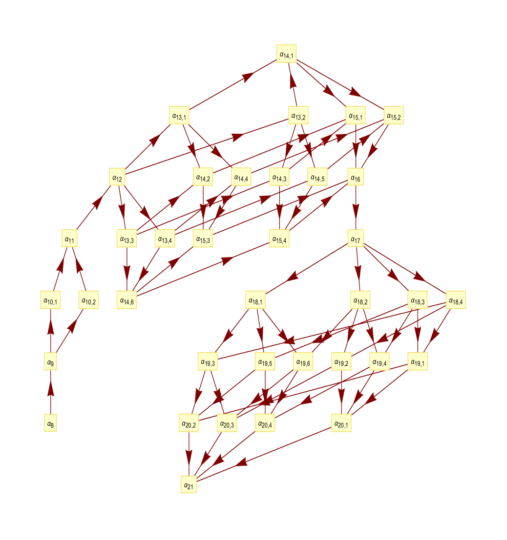
Figure 4. Tree diagram of the optimal sets from $\alpha_{8}$ to $\alpha_{21}$.

In the following theorem, we give the induction formula to determine the optimal sets of $n$-means for any $n\geq 2$.

Theorem 3.10.

For any $n\geq 2$, let $\alpha_{n}:=\{a(i):1\leq i\leq n\}$ be an optimal set of $n$-means, i.e., $\alpha_{n}\in\mathcal{C}_{n}:=\mathcal{C}_{n}(P)$. For $\omega\in I^{\ast}$, let $E(\omega)$ and $E(\omega 1,\omega 2)$ be defined by (5). Set

$$\tilde{E}(a(i)):=\left\{\begin{array}[]{ll}E(\omega)\text{ if }a(i)=a(\omega)\text{ for some }\omega\in I^{\ast},\\ E(\omega 1,\omega 2)\text{ if }a(i)=a(\omega 1,\omega 2)\text{ for some }\omega\in I^{\ast},\end{array}\right.$$

and $W(\alpha_{n}):=\{a(j):a(j)\in\alpha_{n}\text{ and }\tilde{E}(a(j))\geq\tilde{E}(a(i))\text{ for all }1\leq i\leq n\}$. Take any $a(j)\in W(\alpha_{n})$, and write

$$\alpha_{n+1}(a(j)):=\left\{\begin{array}[]{ll}(\alpha_{n}\setminus\{a(j)\})\cup\{a(\omega 1,\omega 2),a(\omega 3)\}\text{ if }a(j)=a(\omega),&\\ (\alpha_{n}\setminus\{a(j)\})\cup\{a(\omega 1),\,a(\omega 2)\}\text{ if }a(j)=a(\omega 1,\omega 2).\end{array}\right.$$

Then $\alpha_{n+1}(a(j))$ is an optimal set of $(n+1)$-means, and the number of such sets is given by

$$\text{card}\Big{(}\bigcup_{\alpha_{n}\in\mathcal{C}_{n}}\{\alpha_{n+1}(a(j)):a(j)\in W(\alpha_{n})\}\Big{)}.$$

Proof.

By Proposition 3.1 and Proposition 3.3, we know that the optimal sets of two- and three-means are $\{a(1,2),a(3)\}$ and $\{a(1),a(2),a(3)\}$. Notice that by Lemma 3.8, we know $E(1,2)>E(3)$. Hence, the theorem is true for $n=2$. For any $n\geq 2$, let us now assume that $\alpha_{n}$ is an optimal set of $n$-means. Let $\alpha_{n}:=\{a(i):1\leq i\leq n\}$. Let $\tilde{E}(a(i))$ and $W(\alpha_{n})$ be defined as in the hypothesis. If $a(j)\not\in W(\alpha_{n})$, i.e., if $a(j)\in\alpha_{n}\setminus W(\alpha_{n})$, then by Lemma 3.9, the error

$$\sum_{a(i)\in(\alpha_{n}\setminus\{a(j)\})}E(a(i))+E(\omega 1,\omega 2)+E(\omega 3)\text{ if }a(j)=a(\omega),$$

or

$$\sum_{a(i)\in(\alpha_{n}\setminus\{a(j)\})}E(a(i))+E(\omega 1)+E(\omega 2)\text{ if }a(j)=a(\omega 1,\omega 2),$$

obtained in this case is strictly greater than the corresponding error obtained in the case when $a(j)\in W(\alpha_{n})$. Hence, for any $a(j)\in W(\alpha_{n})$, the set $\alpha_{n+1}(a(j))$, where

$$\alpha_{n+1}(a(j)):=\left\{\begin{array}[]{ll}(\alpha_{n}\setminus\{a(j)\})\cup\{a(\omega 1,\omega 2),a(\omega 3)\}\text{ if }a(j)=a(\omega),&\\ (\alpha_{n}\setminus\{a(j)\})\cup\{a(\omega 1),\,a(\omega 2)\}\text{ if }a(j)=a(\omega 1,\omega 2).\end{array}\right.$$

is an optimal set of $(n+1)$-means, and the number of such sets is

$$\text{card}\Big{(}\bigcup_{\alpha_{n}\in\mathcal{C}_{n}}\{\alpha_{n+1}(a(j)):a(j)\in W(\alpha_{n})\}\Big{)}.$$

Thus, the proof of the theorem is complete. ∎

Remark 3.11.

Once an optimal set of $n$-means is known, by using (3), the corresponding quantization error can easily be calculated.

Using the induction formula given by Theorem 3.10, we obtain some results and observations about the optimal sets of $n$-means, which are given in the following section.

4. Some results and observations

First, we explain some notations that we are going to use in this section. Recall that the optimal set of one-mean consists of the expected vector of the random vector $X$, and the corresponding quantization error is its variance. Let $\alpha_{n}$ be an optimal set of $n$-means, i.e., $\alpha_{n}\in\mathcal{C}_{n}$, and then for any $a\in\alpha_{n}$, we have $a=a(\omega)$, or $a=a(\omega 1,\omega 2)$ for some $\omega\in I^{k}$, $k\geq 1$. For any $n\geq 2$, if $\text{card}(\mathcal{C}_{n})=k$, we write

$$\mathcal{C}_{n}=\left\{\begin{array}[]{ccc}\{\alpha_{n,1},\alpha_{n,2},\cdots,\alpha_{n,k}\}&\text{ if }k\geq 2,\\ \{\alpha_{n}\}&\text{ if }k=1.\end{array}\right.$$

If $\text{card}(\mathcal{C}_{n})=k$ and $\text{card}(\mathcal{C}_{n+1})=m$, then either $1\leq k\leq m$, or $1\leq m\leq k$ (see Table 1). Moreover, by Theorem 3.10, an optimal set at stage $n$ can contribute multiple distinct optimal sets at stage $n+1$, and multiple distinct optimal sets at stage $n$ can contribute one common optimal set at stage $n+1$; for example from Table 1, one can see that the number of $\alpha_{12}=1$, the number of $\alpha_{13}=4$, the number of $\alpha_{14}=6$, the number of $\alpha_{15}=4$, and the number of $\alpha_{16}=1$.

$n$	$\text{card}(\mathcal{C}_{n})$	$n$	$\text{card}(\mathcal{C}_{n})$	$n$	$\text{card}(\mathcal{C}_{n})$	$n$	$\text{card}(\mathcal{C}_{n})$	$n$	$\text{card}(\mathcal{C}_{n})$	$n$	$\text{card}(\mathcal{C}_{n})$
5	1	18	4	31	6	44	1	57	495	70	56
6	1	19	6	32	4	45	8	58	792	71	28
7	2	20	4	33	1	46	28	59	924	72	8
8	1	21	1	34	6	47	56	60	792	73	1
9	1	22	1	35	15	48	70	61	495	74	1
10	2	23	6	36	20	49	56	62	220	75	12
11	1	24	15	37	15	50	28	63	66	76	66
12	1	25	20	38	6	51	8	64	12	77	220
13	4	26	15	39	1	52	1	65	1	78	495
14	6	27	6	40	1	53	1	66	8	79	792
15	4	28	1	41	4	54	12	67	28	80	924
16	1	29	1	42	6	55	66	68	56	81	792
17	1	30	4	43	4	56	220	69	70	82	495

Table 1. Number of $\alpha_{n}$ in the range $5\leq n\leq 82$.

By $\alpha_{n,i}\rightarrow\alpha_{n+1,j}$, it is meant that the optimal set $\alpha_{n+1,j}$ at stage $n+1$ is obtained from the optimal set $\alpha_{n,i}$ at stage $n$, similar is the meaning for the notations $\alpha_{n}\rightarrow\alpha_{n+1,j}$, or $\alpha_{n,i}\rightarrow\alpha_{n+1}$, for example from Figure 4:

$$\left\{\alpha_{12}\to\alpha_{13,1},\alpha_{12}\to\alpha_{13,2},\alpha_{12}\to\alpha_{13,3},\alpha_{12}\to\alpha_{13,4}\right\},$$

$$\{\left\{\alpha_{13,1}\to\alpha_{14,1},\alpha_{13,1}\to\alpha_{14,2},\alpha_{13,1}\to\alpha_{14,4}\right\},\left\{\alpha_{13,2}\to\alpha_{14,1},\alpha_{13,2}\to\alpha_{14,3},\alpha_{13,2}\to\alpha_{14,5}\right\},$$

$$\left\{\alpha_{13,3}\to\alpha_{14,2},\alpha_{13,3}\to\alpha_{14,3},\alpha_{13,3}\to\alpha_{14,6}\right\},\left\{\alpha_{13,4}\to\alpha_{14,4},\alpha_{13,4}\to\alpha_{14,5},\alpha_{13,4}\to\alpha_{14,6}\right\}\}.$$

Moreover, we see that

$$\alpha_{6} =\{a(1),a(2),a(31),a(32),a(333),a(331,332)\}\text{ with }V_{6}=\frac{3537}{563200}=0.00628018;$$

$$\alpha_{7,1} =\{a(1),a(23),a(21,22),a(31),a(32),a(333),a(331,332)\};$$

$$\alpha_{7,2} =\{a(13),a(11,12),a(2),a(31),a(32),a(333),a(331,332)\}$$

$$\qquad\qquad\text{ with }V_{7}=\frac{1521}{281600}=0.00540128;$$

$$\alpha_{8} =\{a(13),a(11,12),a(23),a(21,22),a(31),a(32),a(333),a(331,332)\}$$

$$\qquad\qquad\text{ with }V_{8}=\frac{2547}{563200}=0.00452237;$$

$$\alpha_{9} =\{a(13),a(11,12),a(23),a(21,22),a(31),a(32),a(333),a(331),a(332)\}$$

$$\qquad\qquad\text{ with }V_{9}=\frac{9171}{2816000}=0.00325675;$$

$$\alpha_{10,1} =\{a(13),a(11,12),a(23),a(21),a(22),a(31),a(32),a(333),a(331),a(332)\};$$

$$\alpha_{10,2} =\{a(13),a(11),a(12),a(23),a(21,22),a(31),a(32),a(333),a(331),a(332)\}$$

$$\qquad\qquad\text{ with }V_{10}=\frac{7191}{2816000}=0.00255362;$$

$$\alpha_{11} =\{a(13),a(11),a(12),a(23),a(21),a(22),a(31),a(32),a(333),a(331),a(332)\}$$

$$\qquad\qquad\text{ with }V_{11}=\frac{5211}{2816000}=0.0018505;$$

and so on.

Remark 4.1.

By Theorem 3.10, we see that to obtain an optimal set of $(n+1)$-means, one needs to know an optimal set of $n$-means. Unlike the probability distribution supported by the classical stretched Sierpiński triangle (see [CR2]), for the probability distribution supported by the nonuniform stretched Sierpiński triangle considered in this paper, to obtain the optimal sets of $n$-means a closed formula is not known yet.

Declaration

Conflicts of interest. We do not have any conflict of interest.

Data availability: No data were used to support this study.

Code availability: Not applicable

Authors’ contributions: Each author contributed equally to this manuscript.

References

- [AW] E.F. Abaya and G.L. Wise, Some remarks on the existence of optimal quantizers, Statistics & Probability Letters, Volume 2, Issue 6, December 1984, Pages 349-351.
- [BW] J.A. Bucklew and G.L. Wise, Multidimensional asymptotic quantization theory with th power distortion measures, IEEE Transactions on Information Theory, 1982, Vol. 28 Issue 2, 239-247.
- [BCDR] P. Biteng, M. Caguiat, T. Dominguez, and M.K. Roychowdhury, Conditional quantization for uniform distributions on line segments and regular polygons, arXiv:2402.08036 [math.PR]
- [BCDRV] P. Biteng, M. Caguiat, D. Deb, M.K. Roychowdhury, and B. Villanueva, Constrained quantization for a uniform distribution, arXiv:2401.01958 [math.DS].
- [CR1] D. Çömez and M.K. Roychowdhury, Quantization for uniform distributions of Cantor dusts on , Topology Proceedings, Volume 56 (2020), Pages 195-218.
- [CR2] D. Çömez and M.K. Roychowdhury, Quantization for uniform distributions on stretched Sierpiński triangles, Monatshefte für Mathematik, Volume 190, Issue 1, 79-100 (2019).
- [DFG] Q. Du, V. Faber and M. Gunzburger, Centroidal Voronoi Tessellations: Applications and Algorithms, SIAM Review, Vol. 41, No. 4 (1999), pp. 637-676.
- [DR] C.P. Dettmann and M.K. Roychowdhury, Quantization for uniform distributions on equilateral triangles, Real Analysis Exchange, Vol. 42(1), 2017, pp. 149-166.
- [GG] A. Gersho and R.M. Gray, Vector quantization and signal compression, Kluwer Academy publishers: Boston, 1992.
- [GKL] R.M. Gray, J.C. Kieffer and Y. Linde, Locally optimal block quantizer design, Information and Control, 45 (1980), pp. 178-198.
- [GL] S. Graf and H. Luschgy, Foundations of quantization for probability distributions, Lecture Notes in Mathematics 1730, Springer, Berlin, 2000.
- [GL1] A. György and T. Linder, On the structure of optimal entropy-constrained scalar quantizers, IEEE transactions on information theory, vol. 48, no. 2, February 2002.
- [GL2] S. Graf and H. Luschgy, The Quantization of the Cantor Distribution, Math. Nachr., 183 (1997), 113-133.
- [GL3] S. Graf and H. Luschgy, Quantization for probability measures with respect to the geometric mean error, Math. Proc. Camb. Phil. Soc. (2004), 136, 687-717.
- [GN] R.M. Gray and D.L. Neuhoff, Quantization, IEEE Transactions on Information Theory, Vol. 44, No. 6, October 1998, 2325-2383.
- [H] J. Hutchinson, Fractals and self-similarity, Indiana Univ. J., 30 (1981), 713-747.
- [HMRT] J. Hansen, I. Marquez, M.K. Roychowdhury, and E. Torres, Quantization coefficients for uniform distributions on the boundaries of regular polygons, Statistics & Probability Letters, Volume 173, June 2021, 109060.
- [HNPR] C. Hamilton, E. Nyanney, M. Pandey, and M.K. Roychowdhury, Conditional constrained and unconstrained quantization for a uniform distribution on a hexagon, arXiv:2401.10987 [math.PR].
- [KNZ] M. Kesseböhmer, A. Niemann and S. Zhu, Quantization dimensions of compactly supported probability measures via Rényi dimensions, Trans. Amer. Math. Soc. (2023).
- [LR] L. Roychowdhury, Optimal quantization for nonuniform Cantor distributions, Journal of Interdisciplinary Mathematics, Vol 22 (2019), pp. 1325-1348.
- [P] D. Pollard, Quantization and the Method of -Means, IEEE Transactions on Information Theory, 28 (1982), 199-205.
- [P1] K. Pötzelberger, The quantization dimension of distributions, Math. Proc. Cambridge Philos. Soc., 131 (2001), 507-519.
- [PR1] M. Pandey and M.K. Roychowdhury, Constrained quantization for probability distributions, arXiv:2305.11110 [math.PR].
- [PR2] M. Pandey and M.K. Roychowdhury, Constrained quantization for the Cantor distribution, arXiv:2306.16653 [math.DS].
- [PR3] M. Pandey and M.K. Roychowdhury, Constrained quantization for a uniform distribution with respect to a family of constraints, arXiv:2309:11498 [math.PR].
- [PR4] M. Pandey and M.K. Roychowdhury, Conditional constrained and unconstrained quantization for probability distributions, arXiv:2312:02965 [math.PR].
- [PR5] M. Pandey and M.K. Roychowdhury, Constrained quantization for the Cantor distribution with a family of constraints, arXiv:2401.01958[math.DS].
- [RR] J. Rosenblatt and M.K. Roychowdhury, Uniform distributions on curves and quantization, Commun. Korean Math. Soc. 38 (2023), No. 2, pp. 431-450.
- [R1] M.K. Roychowdhury, Quantization and centroidal Voronoi tessellations for probability measures on dyadic Cantor sets, Journal of Fractal Geometry, 4 (2017), 127-146.
- [R2] M.K. Roychowdhury, Least upper bound of the exact formula for optimal quantization of some uniform Cantor distributions, Discrete and Continuous Dynamical Systems- Series A, Volume 38, Number 9, September 2018, pp. 4555-4570.
- [R3] M.K. Roychowdhury, Optimal quantization for the Cantor distribution generated by infinite similitudes, Israel Journal of Mathematics 231 (2019), 437-466.
- [Z1] P.L. Zador, Asymptotic Quantization Error of Continuous Signals and the Quantization Dimension, IEEE Transactions on Information Theory, 28 (1982), 139-149.
- [Z2] R. Zam, Lattice Coding for Signals and Networks: A Structured Coding Approach to Quantization, Modulation, and Multiuser Information Theory, Cambridge University Press, 2014.