A New Overview of Secular Period Changes of RR Lyrae stars in M5

Abstract

Secular period variations, $\beta=\dot{P}$, in 76 RR Lyrae stars in the globular cluster M5 are analysed using our most recent CCD $V$ photometry and the historical photometric database available in the literature since 1889. This provides a time baseline of up to 118 years for these variables. The analysis was performed using two independent approaches: first, the classical $O-C$ behaviour of the time of maximum light, and second, via a grid $(P,\beta)$, where the solution producing the minimum scatter in the phased light curve is chosen. The results of the two methods agree satisfactorily. This allowed a new interpretation of the nature of the period changes in many RR Lyrae stars in M5. It is found that in $96\%$ of the stars studied no irregular or stochastic variations need to be claimed, but that $66\%$ of the population shows steady period increases or decreases, and that $34\%$ of the periods seem to have been stable over the last century.

The lack of systematic positive or negative period variations in RR Lyrae stars in other globular clusters is addressed, and the paradigm of period changes being a consequence of stellar evolution is discussed in terms of chemical variations near the stellar core and of multiple stellar populations. In M5 we found a small positive average value of $\beta$ and a small surplus of RRab stars with a period increase. Nevertheless, in M5 we have been able to isolate a group of likely evolved stars that systematically show positive, and in some cases large, period change rates.

1 Introduction

Secular period changes in the RR Lyrae stars (RRLs) of NGC 5904 (M5, or C1516+022 in the IAU nomenclature) ($\alpha=15^{\mbox{\scriptsize h}}18^{\mbox{\scriptsize m}}33.2^{\mbox{\scriptsize s}}$, $\delta=+02\degr 04\arcmin 51.7\arcsec$, J2000; $l=3.85\degr$, $b=+46.80\degr$), have been measured since the pioneering work of Oosterhoff (1941), and in the following seven decades several authors have tackled the problem of estimating the period change rates in pursuit of measurable indications of the stellar evolution on the horizontal branch (HB) accross the instability strip (IS) (Coutts & Sawyer-Hogg 1969, Kukarkin & Kukarkina 1971, Storm et al. 1991, Reid 1996, Szeidl et al. 2011). Photometric studies of M5 are numerous, as are time-series data of its variable stars since 1889 (Bailey 1917), leading to a wealth of resources available for the study of secular period variations.

The most recent and complete study to date of the period variations in the RRLs in M5 was published by Szeidl et al. (2011) (herafter SZ11), who employed a new approach to the $O-C$ method that uses complete light curves rather than a single specific phase. They reported period changes for 86 stars, using a time baseline of about 100 years for the majority of them. While many stars were found to have a uniform period increase or decrease, several very intriguing cases of irregular period variations emerged in that study which are difficult to confront with theoretical expectations. In the present study we have added our most recent CCD time-series of M5 (Arellano Ferro et al. 2016a, hereafter AF16) that extends the time baseline, in many cases, to about 118 years, which have allowed us to re-interpret some of the $O-C$ diagrams, particularly the ones of those peculiar stars.

The present paper is organised as follows; in $\S$ 3 we summarise the previous studies of period changes in M5 and the available data collections in the literature. In $\S$ 4 the methods employed in this work to calculate period change rates are described, the results are reported and a brief discussion of particular cases is included. $\S$ 5 contains a discussion on the lack of systematic period change rates as a consequence of several effects, other than simple evolution, that influence the stellar structure and chemistry and hence the period change rates. A summary of our results and conclusions is given in $\S$ 6.

2 Observations

The most recent $V$ CCD time-series used in this paper to substantially extend the time baseline in many cases to about 118 years, was performed on 11 nights between February 29, 2012 and April 09, 2014 with the 2.0 m telescope at the Indian Astronomical Observatory (IAO), Hanle, India, and have been reported by AF16. A total of 392 images obtained in the Johnson-Kron-Cousins $V$ filter are used here for the purpose of the present analysis. For a full description of observations and the reduction procedure, the reader is referred to AF16.

Table 1: Sources of photometric data and times of maximum light in the RR Lyrae stars of M5.

Authors	years	band	notes
Bailey (1917)	1889-1912	$pg$	1
Shapley (1927)	1917	$pg$	2
Oosterhoff (1941)	1932-35	$pg$	3
Coutts & Sawyer-Hogg (1969)	1936-66	$pg$
Szeidl et al (2011)	1952-1963	$pg$
Szeidl et al (2011)	1971-1993	$pg$
Kukarkin & Kukarkina (1971)			4
Cohen & Gordon (1987)	1986	$B,i$
Storm et al. (1991)	1987	CCD $V$
Cohen & Matthews (1992)	1989	CCD $V$
Brocato et al. (1996)	1989	CCD $V$
Reid (1996)	1991-92	CCD $V$
Kaluzny et al. (1999)	1997	CCD $V$
Present work	2012-14	CCD $V$

1. Times of maximum light were calculated by Kukarkin & Kukarkina (1971), 2: Light curves and times of maximum in Coutts & Sawyer-Hogg (1969) and Coutts (1971). 3: Times of maximum in Coutts & Sawyer-Hogg (1969). 4: No new data are provided but it is a source of times of maximum light.

Table 2: Observed times of maximum light $O$ for RR Lyrae stars in M5 and the corresponding $O-C$ residuals calculated with the given ephemerides for each variable. The sources of either the times of maximum light or the data employed to calculate the times of maximum are coded in column 4 as follows: KK (listed by Kukarkin & Kukarkina 1971); hWil (calculated in this work from Mount Wilson 1917 data published by Coutts & Sawyer-Hogg 1969); hDDO (calculated in this work from DDO data published by Coutts & Sawyer-Hogg 1969); CSH (listed by Coutts & Sawyer-Hogg 1969 from Oosterhoff’s 1941 data); COU (listed by Coutts 1971 from Mount Wilson 1917 data); hOOS (calculated in this work from Oosterhoff’s 1941 data); STO (calculated in this work from data by Storm et al. (1991); BRO (calculated in this work from data by Brocato et al. 1996); KAL (calculated from data by Kaluzny et al. 1999), B24, A49, L24 and P40 (calculated from the data in Table 1 of SZ11); COH (calculated in this work from data by Cohen & Sarajedini 2012); AF16 (calculated from data by AF16). This is an extract from the full table, which is only available with the electronic version of the article (see Supporting Information).

Variable	$P_{0}(days)$	$E_{0}$ (HJD)
V1	0.567513	2456504.1766
$O$ (HJD)	$(O-C)$	No. of Cycles	source
240 0000.+	days
13715.5848	+0.6066	–82004.	KK
16250.4334	+0.5714	–77146.	KK
19535.6214	+0.5443	–70850.	KK
21350.3764	+0.4988	–67372.	KK
21375.9511	+0.5069	–67323	hWil
21424.9782	+0.4883	–67229.	COU
27563.8074	+0.4078	–55464	CSH
27610.2469	+0.4092	–55375.	KK
33858.6369	+0.3190	–43400	hDDO
34154.497	+0.3228	–42833.	B24
36762.3805	+0.2774	–37835.	KK
38071.5434	+0.2613	–35326.	KK
39065.5396	+0.2457	–33421.	KK
39942.1631	+0.2458	–31741.	KK
41007.6310	+0.2144	–29699.	A48
42126.8660	+0.2013	–27554.	L24
42954.4190	+0.1890	–25968.	P40
50578.7717	+0.0878	–11356.	KAL
56063.2547	–0.0059	–845.	AF16
56504.1766	0.0	0.	AF16
56757.2390	–0.0077	+485.	AF16

3 Previous studies of RR Lyrae secular period variations in M5

M5 is one of the most observed globular clusters, and observations since 1889 available in the literature are summarised in Table 1. Including our observations, the baseline spans 118 years, allowing for a detailed analysis of secular period changes of the variables in this cluster. We have digitized all available data listed in Table 1 and, since these older data may be useful for future studies, but time-consuming to put together, we have uploaded them onto the Strasbourg Astronomical Data Center (CDS).

The first-ever study of period variations of RRLs in M5 was performed by Oosterhoff (1941) who, with a time baseline of about 40 years and despite having only three epochs available, 1895-97, 1917 and 1934, was able to detect the period variations in 43 RRab stars (RRc stars were not studied) and to conclude that there was no statistical evidence for preferential period increases in M5. Coutts & Sawyer-Hogg (1969) revisited the cluster adding some 40 years to the time baseline and also concluded that no systematic period variations in the cluster could be argued and that the small period change rates found by them might not necessarily be the result of stellar evolution. To establish this, and considering the time spent by a star on the HB as RR Lyrae, they estimated that the time baseline needed to be extended yet another 30 years. Kukarkin & Kukarkina (1971) extended the period changes analysis for 51 stars adding observations of the Crimean Station of the Sternberg Astronomical Institute including data from 1952 and 1958-1968. They did not publish their observations but listed series of times of maximum light for all the stars in their sample and offered $O-C$ diagrams. They concluded that 27 stars have period increases, 14 period decreases and for 9 the period remains constant. Further period analyses were carried out by Storm et al. (1991) for 10 stars and by Reid (1996) for 30 variables, extending their data time baselines to the 1980s. The most recent and complete analysis of period changes in M5 was published by SZ11, who used a time baseline of about 100 years and supplemented the available data with archival data for the years 1952-1993 not included before. One of the most striking results of this study based on a large sample of 86 RRLs is the large number of variables exhibiting irregular period variations: 50% of the RRc and 34% of the RRab according to these authors. To explain such period variations would be a challenge for the theory of stellar pulsation and evolution across the IS. SZ11 also concluded that there are no preferential period increases or decreases, hence no preferential evolution to the red or to the blue. In the present paper we analyse the period secular variations in a sample of 76 RRLs using two independent methods and revisit the discussion of whether the period variations are the consequence of stellar evolution alone in the HB.

4 Present approaches to the period change rate calculation

We have analysed the period changes in the population of RRLs in M5 by two methods; a) via the classical $O-C$ diagrams constructed from a fixed given ephemeris to predict the times of maximum light and compare them with the observed ones. These diagrams suggest simple period adjustments if the $O-C$ residuals describe a straight line, or allow the determination of the period change rate $\beta=\dot{P}$, if the residuals describe a parabola or a higher order polynomial. b) Searching on a grid $(P,\beta)$, for the pair that produces the light curve with the minimum dispersion. These approaches are described in detail in $\S$ 4.1 and $\S$ 4.2 respectively.

Table 3: New periods and period change rates for RR Lyrae stars in M5. Numbers in parentheses in column 7 are the uncertainties in the last decimal place and correspond to the uncertainty in coefficient $A_{2}$ in eq. 9. Values of $\beta_{0}$ in boldface are the recommended by our analysis.

Variable	Variable	$P_{0}$	$E_{0}$	$E_{0}+A_{0}$	$P_{0}+A_{1}$	$\beta_{0}$	$\beta_{0}$	$P_{0}$	notes
Star ID	Type	(AF16)	(+2 450 000)	(+2 450 000)		$(O-C)$	$(P,\beta)$	$(P,\beta)$
		(days)	(HJD)	(HJD)	(days)	(d Myr-1)	(d Myr-1)	(days)
V1	RRab Bl	0.521794	6757.2390	6757.2354	0.52178651	–0.001(3)	+0.02	0.521787	$b$
V3	RRab	0.600189	6029.2645	6029.2694	0.60018771	+0.040(9)	0.0	0.600186
V4	RRab Bl	0.449647	6046.2142	6046.2148	0.44964950	–0.084(23)	–2.31	0.449556	$a$
V5	RRab	0.545853	6061.3453	6061.3512	0.54584759	–0.306(12)	–	–
V6	RRab	0.548828	5989.4522	5989.4478	0.54882336	–0.113(13)	–0.07	0.548826
V7	RRab	0.494413	5989.4323	5989.4383	0.49441262	+0.227(3)	+0.25	0.494415
V8	RRab Bl	0.546251	5989.3293	5989.3665	0.54625752	+0.474(50)	+0.12:	0.546240	$a$
V9	RRab	0.698899	6063.4105	6063.4203	0.69889415	–0.030(13)	–0.04	0.698893
V11	RRab	0.595897	6046.2751	6046.2751	0.59589193	+0.009(8)	0.0	0.595893	$b$
V12	RRab	0.467699	6046.2434	6046.2467	0.46769709	–0.230(3)	–0.28	0.467695
V13	RRab Bl	0.513133	6046.2579	6046.2299	0.51312442	+0.018(55)	+0.08	0.513127	$b$
V14	RRab Bl	0.487156	6063.2014	6063.2048	0.48715409	–	–	–	$a$
V15	RRc	0.336765	6061.4425	6061.4579	0.33677029	–0.043(1)	+0.03	0.336768	$a$
V16	RRab	0.647632	6029.1907	6756.4814	0.64763260	+0.064(11)	+0.11	0.647635
V17	RRab	0.601390	6312.5181	6312.5207	0.60138522	–0.204(8):	–	–	$a$
V18	RRab Bl	0.463961	6757.2450	6757.2504	0.46395054	–0.007(29)	–	–	$b$
V19	RRab Bl	0.469999	6046.2639	6046.2800	0.4699988	+0.111(4)	–	–	$a$
V20	RRab	0.609473	5987.4631	5987.4773	0.60947601	–0.021(6)	–0.06	0.609473	$b$
V24	RRab Bl	0.478439	6029.3187	6029.3310	0.47843694	–0.327(11)	–	–	$a$
V25	RRab	0.507525	5987.3835	5087.3861	0.50756321	+0.933(94)	+4.01	0.507685	$a$
V26	RRab Bl	0.622561	5989.4356	5989.4459	0.62256400	–0.001(20)	0.0	0.622564	$b$
V27	RRab	0.470322	6063.3866	6063.3959	0.47033603	–0.301(6)	$-$	–
V28	RRab Bl	0.543877	6312.5122	–	–	–	–0.16:	0.543922	$a$
V30	RRab	0.592178	5987.4673	5987.4708	0.59217587	–0.007(21)	0.0	0.592176	$b$
V31	RRc bump	0.300580	6046.2639	6046.2466	0.30058184	–0.012(1)	–0.05	0.300580	$a$
V32	RRab	0.457785	5989.4255	5989.4275	0.45778643	–0.004(4)	–	–	$b$
V33	RRab	0.501481	5989.3506	5989.3502	0.50148223	+0.068(7)	+0.09	0.501481
V34	RRab	0.56810	6061.2497	6061.2499	0.56814325	0.003(9)	0.0	0.568145	$b$
V35	RRc bump	0.308217	6063.2209	–	–	–	–	–	$a$
V36	RRab	0.627725	6061.1878	6061.1759	0.62772336	+0.038(12)	–	–	$a$
V37	RRab	0.488801	6029.3187	6029.3184	0.48880064	+0.089(3)	+0.12	0.488802
V38	RRab	0.470422	6504.2422	6504.2582	0.47042828	–0.018(49)	–	–	$a,b$
V39	RRab	0.589037	6063.3327	6063.3305	0.58904270	+0.081(6)	+0.11	0.589044
V40	RRc Bl	0.317327	6063.1929	6063.2066	0.31732968	–0.005(5)	–0.01	0.317329	$b$
V41	RRab	0.488572	6061.3027	6061.3054	0.48856722	–0.078(12)	–0.04	0.488569	$a$
V43	RRab	0.660226	6029.2970	6757.4952	0.66022986	+0.023(11)	0.0	0.660229
V44	RRc	0.329599	5987.4916	5987.4848	0.32960270	+0.006(12)	0.0	0.329603	$b$
V45	RRab Bl	0.616636	6061.3946	6061.3870	0.61663865	+0.027(5)	+0.01	0.616638
V47	RRab	0.539730	6757.2200	6312.4917	0.53972813	0.022(12)	0.0	0.539728	$b$
V52	RRab	0.501541	6029.2645	6029.2705	0.50154260	+0.044(23):	–	–	$a$
V53	RRc	0.373519	5987.5209	5987.5172	0.37351709	0.0	–	–	$a,b$
V54	RRab	0.454115	5989.3176	5989.3192	0.45411516	+0.045(7)	–	–	$a$
V55	RRc Bl	0.328903	6504.1925	6504.1933	0.32890264	+0.058(8)	+0.07	0.328903
V56	RRab Bl	0.534690	6061.3186	6029.2424	0.53469980	+0.166(16)	+0.20	0.534701	$a$
V57	RRc	0.284697	6046.2434	6046.2467	0.28469423	–0.094(14)	–0.01	0.284689
V59	RRab	0.542025	6061.2807	6061.2820	0.54202707	+0.016(3)	–0.03	0.542024
V60	RRc bump	0.285236	6504.1518	6504.1550	0.28523571	–0.018(6)	–0.04	0.285235
V61	RRab	0.568642	6061.4250	6061.4286	0.56864272	+0.266(5)	+0.25	0.568642
V62	RRc bump	0.281417	5989.3176	5989.3057	0.28142735	+0.200(9)	–	–	$a$
V63	RRab Bl	0.497686	6756.3534	6046.1731	0.49768368	+0.065(9)	+0.06	0.497683
V64	RRab	0.544489	6062.1833	6062.1804	0.54449142	–0.161(27)	–0.13	0.544493
V65	RRab Bl	0.480664	5989.4389	5989.4474	0.48067521	+0.214(7):	–	0.480672	$a,b$
V74	RRab	0.453984	6061.3915	6061.3934	0.45398467	–0.119(3)	–0.12	0.453985
V77	RRab	0.845158	6061.3518	6061.3484	0.84514463	+0.340(21)	+0.32	0.845145
V78	RRc	0.264820	5989.5204	5989.5341	0.26481743	–0.003(3)	0.0	0.264817	$b$
V79	RRc	0.333139	6046.2326	6046.2411	0.33313845	–0.012(4)	–	–	$b$
V80	RRc	0.336542	6046.2751	6046.2843	0.33654488	+0.123(7)	–	–	$a$

^a: There is a comment for this star in $\S$ 4.4. A colon after the value of $\beta$ indicates particularly uncertain values.
^b: All these stars display a linear $O-C$ diagram and in fact $\beta$ is not significantly different from zero. Therfore, we recommend a value of $\beta$ = 0.0

Table 3: Continued

Variable	Variable	$P_{0}$	$E_{0}$	$E_{0}+A_{0}$	$P_{0}+A_{1}$	$\beta_{0}$	$\beta_{0}$	$P_{0}$	notes
Star ID	Type	(AF16)	(+2 450 000)	(+2 450 000)		$(O-C)$	$(P,\beta)$	$(P,\beta)$
		(days)	(HJD)	(HJD)	(days)	(d Myr-1)	(d Myr-1)	(days)
V81	RRab	0.557271	6504.2422	6504.2393	0.55726945	–0.562(9)	–	–
V82	RRab	0.558435	6063.2014	6063.2038	0.55843655	–0.051(91)	–0.23	0.558433	$b$
V83	RRab	0.553307	6061.4320	6061.4372	0.55330724	–0.008(6)	–	–	$b$
V85	RRab Bl	0.527535	6061.3804	6061.3804	0.52752587	–0.234(12)	+0.71	0.527537	$a$
V86	RRab	0.567513	6504.1925	6504.1916	0.56751027	–0.065(9)	–	–	$a$
V87	RRab	0.738421	6061.2186	6061.2050	0.73842323	+0.369(14)	+0.35	0.738423
V88	RRc	0.328090	5989.5102	5989.5271	0.32808564	–0.024(21)	–0.45	0.328080	$b$
V89	RRab	0.558443	6063.1970	6063.1985	0.55844471	+0.060(58)	–0.04	0.558445
V90	RRab	0.557168	6061.3518	6061.3482	0.55716550	+0.114(8)	+0.10	0.557165
V91	RRab	0.584945	6063.4183	6063.4085	0.58494285	+0.011(27)	0.0	0.584943	$b$
V92	RRab Bl	0.463388	6061.1878	6061.1781	0.46338677	+0.025(19)	–0.87:	0.463351	$a,b$
V93	RRab	0.552300	5987.4505	–	–	–	–	–	$a$
V94	RRab	0.531327	6061.2497	6061.2475	0.53132796	0.0	–	–	$a,b$
V95	RRc bump	0.290832	6061.3613	–	0.29083223	0.0	+2.15	0.290833	$a,b$
V96	RRab	0.512255	6312.48	–	0.512255	0.0	+0.04	0.512255	$a,b$
V97	RRab Bl	0.544656	5987.3747	5987.3660	0.54464622	–0.134(35)	+0.85:	0.544654	$a$
V98	RRc	0.306360	6063.4216	6063.4111	0.30636289	+0.022(14)	–	–	$a$
V99	RRc Bl	0.321336	6061.2186	6061.2059	0.32134529	+0.159(28)	–0.03	0.321344	$a$
V100	RRc	0.294365	6504.1849	9395.2457	0.29436548	0.0	–	–	$a,b$

^a: There is a comment for this star in $\S$ 4.4. A colon after the value of $\beta$ indicates particularly uncertain values.
^b: All these stars display a linear $O-C$ diagram and in fact $\beta$ is not significantly different from zero. Therfore, we recommend a value of $\beta$ = 0.0

4.1 The $O-C$ method

The observed minus the calculated ($O-C$) residuals of a given feature in the light curve, as an indication of miscalculations or authentic variations of the pulsation or orbital period, using a single given phase of the light curve as a reference, is a standard approach that has been in use for many decades for example in Cepheids, RR Lyrae and contact binary stars (e.g. Arellano Ferro et al. 1997; Coutts & Sawyer-Hogg 1969; Reid 1996; Lee et al. 2011). It is convenient to select a feature that facilitates the accurate determination of the phase. For RRab stars a good selection is the time of maximum brightness, which is well constrained, as opposed to the longer-lasting time of minimum or mean light. To predict the time of maximum one adopts an ephemeris of the form

$$C=E_{0}+P_{0}N,$$ (1)

where $E_{0}$ is an adopted origin or epoch, $P_{0}$ is the period at $E_{0}$ and $N$ is the number of cycles elapsed between $E_{0}$ and $C$. An initial estimate of the number of cycles between the observed time of maximum $O$ and the reference $E_{0}$ is simply,

$$N=\left\lfloor\frac{(O-E_{0})}{P_{0}}\right\rfloor,$$ (2)

where the incomplete brackets indicate the rounding down to the nearest integer. However, we must note that if the time between $E_{0}$ and the observed time of maximum $O$ is much larger than the period, and the period change rate is large enough, the $O-C$ difference can exceed one or more cycles and then one must correct for these extra cycles to obtain a correct $O-C$ diagram. This exercise may prove difficult if there are large gaps in the time-series but is rather straightforward otherwise, as is the present case of M5.

A plot of the number of cycles $N$ vs $O-C$, usually referred to as an $O-C$ diagram, and its appearance evidence a secular variation of the period (mostly parabolic but a higher order is also possible) or the fact that the period $P_{0}$ used in the ephemerides is wrong, which produces a linear $O-C$ diagram.

Let us assume the intitial model a cubic distribution of the $O-C$ residuals as function of time, represented by the number of cycles $N$ elapsed relative to the initial epoch $E_{0}$. The linear and quadratic cases are then particular solutions of this more general representation:

$$O-C=A_{0}+A_{1}N+A_{2}N^{2}+A_{3}N^{3},$$ (3)

or,

$$O=(E_{0}+A_{0})+(P_{0}+A_{1})N+A_{2}N^{2}+A_{3}N^{3}.$$ (4)

From eq.4 it is clear that $E_{0}+A_{0}$ is the corrected epoch for a given fit and that $P_{0}+A_{1}$ is the corrected period at that epoch.

Taking the derivative allows us to calculate the period at any given $N$,

$$P(N)=\frac{dO}{dN}=(A_{1}+P_{0})+2A_{2}N+3A_{3}N^{2},$$ (5)

and,

$$\beta\equiv\dot{P}=\frac{dP}{dt}=2A_{2}\frac{dN}{dt}+6A_{3}N\frac{dN}{dt}.$$ (6)

Since the time elapsed to a given epoch is the period times the number of cycles, $t=PN$, then $\beta$ at a given epoch $N$ and its secular variation $\dot{\beta}$ can be written respectively as

$$\beta=\frac{2A_{2}}{P}+\frac{6A_{3}N}{P},$$ (7)

and

$$\dot{\beta}=\frac{6A_{3}}{P^{2}}-\frac{\beta}{P^{2}}(2A_{2}+6A_{3}N).$$ (8)

Eq. 8 represents the variation of period change rate at a given time $N$. For $N=0$ and $P=P_{0}$ we get,

$$\beta=\beta_{0}=\frac{2A_{2}}{P_{0}},$$ (9)

and

$$\dot{\beta_{0}}=\frac{6A_{3}}{P_{0}^{2}}-\frac{4A_{2}^{2}}{P_{0}^{3}}.$$ (10)

If we set $A_{2}=A_{3}=0$ in eq. 4 we would be dealing with the linear case were the original estimate of the period $P_{0}$ should be corrected to $P_{0}+A_{1}$.

We have used the available data in the literature since 1889 to build up a collection of as many times of maximum light of as many RRLs as possible. Some authors have already published times of maximum for some variables in M5 (e.g. Coutts 1971, Kukarkin & Kukarkina 1971), and in these cases we have adopted their values. For other authors, we have used the published photometric data to estimate the times of maximum. When necessary we have transformed Julian days into heliocentric Julian days. The complete collection of the times of maximum for each star is given in Table 2, of which we show here just a small portion since the full table is only available in electronic form. To calculate the $O-C$ residuals as described above, we adopted for each studied variable the ephemerides given by AF16 in their table 3, and also listed in columns 3 and 4 of the present Table 3.

The resulting $O-C$ diagrams are shown in Fig. 1 for every variable with observed times of maximum. For stars numbered above V100 we have not found published photometry in the literature, thus the times of maximum light reported in Table 2 are those that we have calculated from the data available in AF16; although this limitation inhibits any period change analysis at present, we publish those times of maximum for the benefit of any possible future analysis. Therefore, Table 3 and Fig. 1 include only up to variable V100.

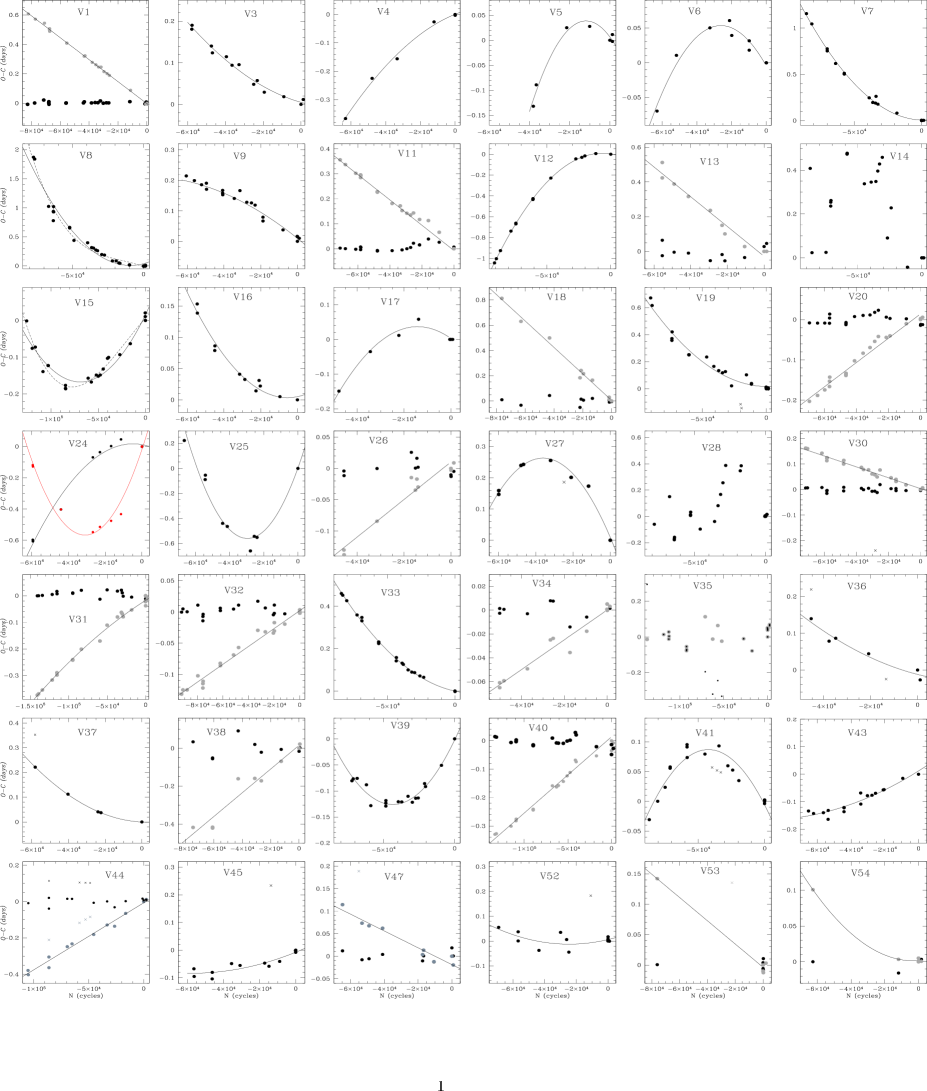
Figure 1: $O-C$ diagrams. For stars with linear distributions we have plotted with gray symbols the distribution using the ephemerides listed by AF16 (columns 3 and 4 in Table 3) and with black symbols the distribution after the refined ephemerides (columns 5 and 6 in Table 3). Those $O-C$ residuals plotted with an X symbol were not considered in the fits.

Figure 1: Continued

4.2 The $(P,\beta)$ grid approach

When studying the period variations of variable stars it is common that the available data do not span long enough or that the number of times of maximum light is small, making it difficult to approach the problem via the classical $O-C$ residuals analysis. Alternatively, we have recently used recently the approach introduced by Kains et al. (2015) to calculate $\beta$ for a sample of RRLs in NGC 4590 and also employed for NGC 6229 (Arellano Ferro et al. 2015b); we briefly summarise this method here. The period change can be represented as,

$$P(t)=P_{0}+\beta(t-E),$$ (11)

where $\beta$ is the period change rate, and $P_{0}$ is the period at the epoch $E$. The number of cycles at time $t$ elapsed since the epoch $E$ is:

$$N_{E}=\int_{E}^{t}\frac{dx}{P(x)}=\frac{1}{\beta}{\rm ln}[1+\frac{\beta}{P_{0}}(t-E)],$$ (12)

hence the phase at time $t$ can be calculated as

$$\phi(t)=N_{E}-{\left\lfloor N_{E}\right\rfloor}.$$ (13)

Then we construct a grid $(P,\beta)$ with values in steps of $10^{-6}d$ and 0.01 d Myr^-1 in $P$ and $\beta$ respectively, around a given starting period $P_{0}$, and examine the light curve dispersions for each pair. We choose as a solution the one that produces the minimum dispersion of all the data sets phased simultaneously. Since the penalty for increasing dispersion depends on the number of data, this method works best for variable stars with many observations, as it can otherwise find many local minima in the grid. We also note that when a solution with $\beta$=0 was among the 10 light curves with the least dispersion, we adopted this solution, corresponding to a simple period adjustment.

A comparison and a discussion of the grid results with the ones from the $O-C$ method and those obtained by SZ11 are given in $\S$ 4.4.

4.3 Phasing of the light curves with secular period change

Figure 2: Three selected examples of light curve phasing with ephemerides including the secular period variation parameters described in $\S$ 4.1 and given in Table 3 (top panels). In the bottom panels the light curves were phased with a constant period ephemerides, which makes evident the lack of proper phasing of the several data sets involved (see $\S$ 4.3 for a discussion).

Once a period change rate has been calculated, a natural test is to phase the light curve given the new ephemeris. For the sake of brevity we do not plot all the stars in Table 3 but show three representative examples in Fig. 2. In the lower panels we show the light curve of all available data phases with a constant period ephemeris (columns 3 and 4 in Table 3). The upper panels show the light curve phase with the period change ephemerides (columns 5, 6 and 7 in Table 3) according to eqs. 4, 5 and 6. V12 is an RRab star for which the value of $\beta$ found by the $O-C$ and the grid method agree and the new phasing is correct. For the RRab V81 the grid method failed in finding an optimal solution. The $O-C$ approach finds a period change rate that phases well the available data. For the RRc V62 the grid method did not converge and although the $\beta$ value from the $O-C$ approach improves the light curve phasing, it does not produce a perfectly phased light curve for all the data sets. We believe this is a reflection of the scatter and uncertainties inherent to the $O-C$ diagram. The grid method is very sensitive to the dispersion of the light curves involved in the calculation and hence in some instances we could not derive a convincing value of $\beta$. In Table 3 we mark with a colon those values of $\beta$ that we consider to be particularly uncertain.

4.4 Discussion on the period changes and individual cases

From the $O-C$ diagrams in Fig.1 it is clear that the majority of the stars display either a linear or a quadratic distribution. The linear cases imply a constant period whose appropriate value is estimated by requiring that the slope of the line be zero. The refined ephemerides are given in columns 5 and 6 of Table 3 as $E_{0}+A_{0}$ and $P_{0}+A_{1}$ (see eq. 4). These linear cases are all labelled $b$ in the last column of Table 3 and for homogeneity we calculated their $\beta$ by adjusting a parabola to the $O-C$ distribution; as can be seen in all these cases $\beta$ is not significantly different from zero, hence we conclude that their period has remained constant for the last century. For a few stars whose apparent linear solution depends on a very low number of points, we have adopted $\beta$=0, but have refrained from performing any further statistics (e.g. V53, V94, V95, V96 and V100). Similarly, some quadratic solutions based on a low number of epochs are listed in Table 3 as a reference but they are not highlighted since a solution can easily change by adopting a slightly different number of cycles, see the explicit examples of V85 and V97 in Fig. 1. The boldface highlighted values of $\beta$ in Table 3 are our recommended values as they are better estimated and produce a good phasing of the combined light curves. The uncertainties given in parentheses after the $(O-C)$ results were calculated from the uncertainty of coefficient $A_{2}$ following eq. 9 and neglecting the period uncertainty. The resulting $P$ and $\beta$ from the grid approach ($\S$ 4.2) are listed in column 8. The $(P,\beta)$ method is a useful independent check on the values found with the $(O-C)$ method. However, because it relies on the comparison of the string length of phased light curves, rather than on a standard goodness-of-fit statistic, it is difficult to obtain rigorous estimates of the uncertainties associated with the values of $\beta$ yielded by the $(P,\beta)$ method. Such estimates are possible, but require detailed Monte Carlo simulations that are beyond the scope of this study.

Except for a few cases with an unclear solution, mostly due to the scarcity of times of maximum light or, in three cases (V14, V28 and V35) due to an irregular distribution of the $O-C$ residuals, all the stars studied here show either a smooth period change or the period appears to be constant over the last century. We found three cases where the $O-C$ residuals are best represented by a cubic equation, implying a secular variation of the period change rate $\beta$ (V8, V15 and V80). We do not confirm the irregular period variations reported by SZ11 in at least one third of the stars studied by both teams. We attribute this to the fact that in long time baseline data sets and for stars with short periods, like RRLs, the $O-C$ residuals can easily exceed one or two cycles and then the number of cycles might be miscounted. We have paid special attention to the proper counting of cycles elapsed since the reference epoch in the adopted ephemerides and we could always, or almost always, make the residuals to be consistent with a linear or a parabolic distribution, which in turn are easier to understand on evolutionary grounds than the stochastic oscillations in the $O-C$ diagrams.

In what follows we compare the resulting values of $\beta$ obtained from the two approaches described in $\S$ 4.1 and $\S$ 4.2, and subsequently with the results of SZ11. Finally, we will highlight and comment on some individual peculiar cases.

4.4.1 $O-C$ vs $(P,\beta)$

In Fig. 3 the $\beta$ values from the $O-C$ and $(P,\beta)$ approaches are compared. We were able to estimate $\beta$ by the two independent methods for 38 stars. The agreement of the two methods is generally very good, within 0.05 d Myr^-1 for 32 stars, between 0.08 and 0.13 d Myr^-1 for 3 stars, and there are 3 outliers; V8 in the plot plus V4 and V25 not shown in the figure. For 26 stars the $O-C$ diagrams suggest a constant period which could be refined by fitting a straight line and then calculating $P_{0}+A_{1}$ (see eq. 5), these have a label $b$ in the notes column of Table 3. For some of these stars (V1, V13, V20, V40 and V96) the $(P,\beta)$ approach also suggested a small period change rate. These stars are plotted with green symbols in Fig. 3. We call attention to those stars with discrepant values of $\beta$ from the two approaches (V82, V85, V88, V95, V97, V99). These stars either show prominent Blazhko amplitude modulations (AF16), and/or have very few epochs (Fig. 1) or have a strong bump near the maximum light (V95, V99); see their light curves in AF16); all these circumstances act against a good determination of the period change rate. We have not plotted in Fig. 1 those stars with sparse data. Further comments on these stars are found in $\S$ 4.4.3.

4.4.2 Comparison with SZ11

An overall comparison with the results of SZ11 and a discussion of some specific discrepant cases are of interest and they will be addressed below. The comparison is graphically displayed in Fig. 4.

There are 80 stars in common in Table 3 and SZ11. For 27 of them our $\beta$ values agree within 0.03 d Myr^-1 and for 7 the differences are between 0.05 and 0.18 d Myr^-1. These cases are plotted with filled circles in Fig. 4. We also note that for 13 stars for which our $O-C$ approach suggested a clear period variation, SZ11 do not report a value of $\beta$ generally because their $O-C$ diagrams show an irregular variation. We have found that in the majority of these cases a proper counting of cycles leads to a homogeneous parabolic $O-C$ distribution and hence to a clear value of $\beta$. To show the range of $\beta$ implied by these stars, we have plotted them as open symbols in Fig. 4. Likewise for 7 stars we found a linear $O-C$ distribution instead of the irregular one of SZ11.

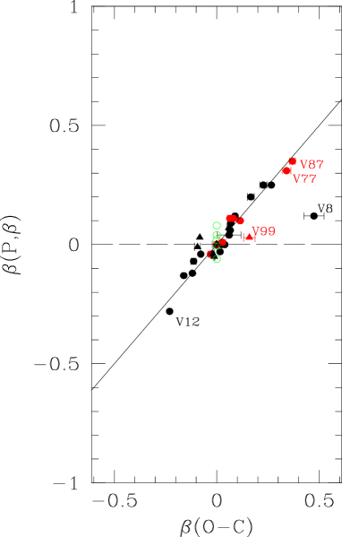
Figure 3: Comparison of period change rates $\beta$ (in d Myr^-1) from the $O-C$ approach described in $\S$ 4.1 and the grid $(P,\beta)$ method of $\S$ 4.2. Circles and triangles represent RRab and RRc stars respectively. Red circles represent evolved stars identified by AF16 (see text for a discussion). Error bars on $\beta(O-C)$ values are drawn only when they are noticeably bigger than the symbol size. Open green symbols are those stars with a constant period ($\beta=0$) according to the $O-C$ approach, but probably in most cases due to the presence of strong Blazhko and/or scattered and scarce data, a non-zero value of $\beta$ was found by the grid $(P,\beta)$ approach. See $\S$ 4.4 for a discussion of individual stars.

For 10 stars, both SZ11 and us found no significant secular period variations, i.e. $\beta\sim 0.$ These are not represented in Fig. 4 and most of them are the ones with straight $O-C$ residuals distribution in Fig. 1.

4.4.3 Comments on individual peculiar cases

The following individual cases deserve specific comments:

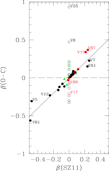
Figure 4: Comparison of period change rates $\beta$ from SZ11 and the $O-C$ approach in the present paper for stars in common. Circles and triangles represent RRab and RRc stars respectively. Red circles represent evolved stars according to the amplitude-period diagram of AF16 (see $\S$ 5 for a discussion). Open symbols are used for star with a value of $\beta$ in the present work but not calculated by SZ11, mostly because they were found by SZ11 with a peculiar $O-C$ residuals distribution; they are plotted at $\beta(\rm{SZ11})=0$.

V4, V17, V19, V24, V25, V27, V52, V56, V62, V65, V80, V85, V98. For these stars SZ11 found a peculiar $O-C$ distribution. Contrary to this we found a clear parabolic distribution indicating a smooth secular period variation. We attribute this difference to the counting of cycles that, if it is not properly made, may cause that the $O-C$ diagram can show peculiar deformations.

V11, V18, V38, V40, V47, V88, V92. These are the stars with a linear distribution of the $O-C$ residuals in Fig. 1 but found with an irregular distribution by SZ11.

V1, V13, V20, V30, V32, V34, V78, V79, V83, V91. For these stars both SZ11 and this work agree that their period is not undergoing a secular variation.

V8, V15, V80. These stars show a period increase in both the present work and in SZ11. We found that their $O-C$ diagrams admit a parabola or a third degree polynomial, which implies a variable period change rate. A similar result is found by SZ11 for V8 but no value of $\beta$ is reported. We were not able to find a good phasing for V8 with the $(P,\beta)$ approach thus its value of $\beta$ in Table 3 is marked with a colon.

V4, V25. The very large values of $\beta$, $-2.31$d Myr^-1 for V4 and $+4.01$d Myr^-1 for V25, determined by the $(P,\beta)$ method (not shown in Fig. 3) are at odds with those obtained by the $O-C$ method. These two stars show very clear and prominent Blazhko amplitude and phase modulations (see the light curves in AF16) which make the determination of the period change, by both the $(O-C)$ and $(P,\beta)$ methods very uncertain.

V14, V35. These are examples of irregular $O-C$ diagrams according to SZ11. Our $O-C$ distribution confirms this. We found no way to reconcile the residuals with a homogeneous variation. The RRab V14 is also a Blazhko variable and the RRc V35 displays a prominent bump near maximum light which has probably influenced the historical determinations of the times of maximum light. Some evidence of Blazhko modulations have also been found in V35 (see the light curves in AF16). Depending on the cycle counting, especially in data from around the 1960’s, one could interpret the $O-C$ diagram as having a constant period, in agreement with the result of SZ11, or as having an abrupt period change at that time (gray and black dots in Fig. 3 respectively). It is interesting to note that the $(P,\beta)$ approach suggests $\beta$=+1.750, a very large value which may be a spurious result driven by the presence of the bump and the Blazhko modulations. Other regions of the P-$\beta$ plane were explored in search of other possible solutions but no convincing phasing was found.

V24. We found a $O-C$ distribution similar to the one of SZ11. It can be approximated by an upward parabola (red in Fig. 4), in this case the resulting value of $\beta$ (+0.868 d Myr^-1) would be the largest in M5, similar to the case of V25. We note however that through an appropriate count of cycles one could accomodate a downward parabola (black in Fig. 4) with a negative value of $\beta$ ($-0.327$ d Myr^-1). The $(P,\beta)$ method failed to find a convergent solution for this star. Thus, we are not conclusive about the period variations of this star.

V28. As for V14 and V35 we could not reconcile our $O-C$ diagram with a homogeneus period change but found an irregular distribution. SZ11 found a neat $O-C$ diagram that would be consistent with a period decrease, they reported $\beta$= -0.236 d Myr^-1. The $(P,\beta)$ approach leads to $\beta$= -0.16 d Myr^-1 in reasonable agreement with SZ11. V28 has a very strong amplitude Blazhko modulation (AF16) which apparently has altered the times of maximum sufficiently to produce the irregular $O-C$ diagram.

V31. Although this star was found by SZ11 to have a constant period, we found that a very gentle downward parabola can be admitted, as opposed to a tilted straight line, which corresponds to a mild period decrease with $\beta=-0.012$ d Myr^-1.

V36. No period variation was found by SZ11. Our $O-C$ diagram might also admit a small period increase with $\beta=+0.03$ d Myr^-1 represented by a soft upward parabola.

V38. This apparently constant period star has a scattered $O-C$ diagram probably due to its Blazhko nature detected by Jurcsik et al. (2011).

V41. We, like SZ11, find a downward parabola and a very similar value of $\beta$. However we note that we had to ignore three maxima from Kukarkin & Kukarkina (1971) that seemed discordant.

V62, V65. Both $O-C$ diagrams of SZ11 and ours in Fig 4 show small discrepancies about the parabola of these otherwise period-increasing stars. SZ11 do not report a value of $\beta$. In fact V65 could also be interpreted as a constant period variable if the four oldest data points were shifted one cycle downwards (segmented line in Fig. 1).

V53, V54, V85, V86, V92-V100. These stars have very few observed times of maximum light, and consequently the $O-C$ solutions are not always clear and often depend on one or two points, e.g. see the cases of V85 and V86 where the removal of one datum can change the solution from quadratic to linear. For V92 and V97 we were unable to find a proper phasing of the data by the $(P,\beta)$ approach and the reported $\beta$ are marked with a colon. In Table 3 and Fig. 1 we have suggested likely solutions for these stars, however inconsistencies with SZ11 should not be either surprising or significant. These stars will not be included in the overall period change statistics of the cluster. V53 and V86 were not included by SZ11.

We note that despite these adverse circumstances one of the competing solutions produce a reasonable phasing of the light curve, as can be seen in Fig.

Further comments on V82, V85, V88, V95, V97, V99. It has been pointed out in $\S$ 4.4.1 that data on these stars are sparse, and that they show either prominent Blazhko modulations and/or a bump near the maximum light (AF16), hence it is difficult to be conclusive on their secular period behaviour. In Fig. 5 the light curves phased with the two competing results are displayed. In spite that one of the solutions produces a reasonable phasing, we warn that these cases should be considered as marginal until more data become available.

Figure 5: Phasing of the light curves of stars with discrepant values of $\beta$ values from the $(O-C)$ (top panels) and the $(P,\beta)$ (bottom panels) approaches. One of the competing solutions seems to produce a proper phasing of the light curve. Refer to $\S$ 4.4.3 for a discussion.

5 Period changes and evolution in the HB

It is clear that as stars evolve across the instability strip, their pulsation period should increase if evolution is to the red and decrease if evolution is to the blue. However, it is also understood now that evolution is most likely not the only reason for period variations and stochastic variations have also been proposed (Balazs-Detre & Detre 1965). In fact several authors have found irregular and complicated $O-C$ diagrams (e.g. SZ11, Jurcsik et al. 2001), which indeed would be difficult to reconcile with evolution exclusively. Sweigart & Renzini (1979) suggested that mixing events in the core of a star at the HB may alter the hydrostatic structure and pulsation period and that a small transfer of helium inwards at the semiconvective zone, near the convective core boundary, can be responsible for period changes, either positive, negative, or irregular. However, we note that at least in the case of M5, there is no need to claim for irregular period variations since an improper counting of cycles, particularly in long time baseline sets of times of maximum light, may be responsible for those apparent irregularities, with the probable exception of V14 and V35.

It has been in the interest of several authors in the past to infer evolutionary properties accross the instability strip by searching for preferential directions of evolution as indicated by the secular period changes in RRLs. A preferential period variation through the IS, in either direction, seems however to be improbable. There are several reasons for this. Growing evidence of several stellar populations coexisting in a given globular cluster have been put forward in recent years, both theoretically and observationally as well as on spectroscopic (Carretta et al. 2010; Gratton et al. 2012) and photometric (e.g. Piotto et al. 2007, Sbordone et al. 2011, Alonso-García et al. 2015) grounds. The presence of multiple populations, and their role in the structure of the IS at the horizontal branch, have recently been discussed by Jang et al. (2014) and Jang & Lee (2015) in connection with the origin of the Oosterhoff types dichotomy. They conclude that RRab-type stars in OoII clusters belong to a second generation with the helium abundance $Y$ slightly increased and carbon, nitrogen, and oxigen (CNO) noticeably enhanced which produce more luminous and redder stars, therefore with longer periods; in OoI clusters the RRab stars are members of the less luminous first generation. However, this scenario, that aims to explain the Oosterhoff dichotomy, does not account for the non-preferential distribution of increasing and decreasing periods in a given globular cluster. Thorough and extensive investigations on the secular period change rates, $\beta$, in a few clusters have been carried out and the averages are not significantly different from zero; for M3 Corwin & Carney (2001) found an overall average of +0.004$\pm$0.335 for 37 RRLs and also Jurcsik et al. (2012) found a small positive value of about +0.01 for some 54 RRLs. For M15 Silbermann & Smith (1995) found an average of +0.06$\pm$0.24 for 27 RRLs and excluding the double mode or RRd pulsators also Smith & Wesselink (1977) found an average of +0.11$\pm$0.36; for NGC 4590 Kains et al. (2015) found an average of +0.02$\pm$0.57 for 14 stars; NGC 7006 Wehlau, Slawson & Nemec (1999) found +0.03$\pm$0.14 for stars; for M28 Wehlau et al. (1986) found -0.06$\pm$0.29 for 11 stars; for M14 Wehlau & Froelich (1994) found +0.04$\pm$0.43 for 35 stars. The case with the largest positive average $\beta$ is $\omega$ Cen (Jurcsik et al. 2001 their table 6) for which we calculate +0.170$\pm$0.561. All the above cited uncertainties correspond to the standard deviation of the mean. The case of IC4499 (Kunder et al. 2011) comes a bit as a surprise since the average +0.29$\pm$0.60 from 39 stars (their Table 1 without three extreme cases) is found despite of not having a very blue HB ($\cal L$=+0.11). Also, in all the above studies no significant differences were found in the average values of $\beta$ for the population of RRab and RRc stars.

On theoretical grounds, Lee (1991) demonstrated that in globular clusters with blue HB morphologies, the average rate of period change $\beta$ would become increasingly large but it will be small on average for the RRLs in globular clusters with reddest HB’s (see his figure 4). An updated version of this correlation, provided by Catelan & Smith (2015) (their figure 6.16), supplemented with new theoretical calculations and more empirical results confirms the trend. However, on empirical grounds the trend of increasing $\beta$ with very blue HB types is driven primarily by $\omega$ Cen [a peculiar cluster with a large star-to-star spread of heavy element abundances as pointed out by Catelan & Smith (2015) and Valcarce & Catelan (2011)], but also by M3 and M28, and (to some extent) M22. Further studies of secular period variations in globular cluters with (very) blue HB types are strongly encouraged, as this would enable a better investigation of the possible connection between period change rates and evolution along the HB.

For M5 several authors have concluded that the averages of period changes do not show significantly preferential increasing or decreasing periods (e.g. Reid 1996, Coutts & Sawyer-Hogg 1969, SZ11). SZ11 found an overall average of -0.006$\pm$0.162 for 55 stars. From our Table 3 we can see that out of the 76 stars studied, constant periods are evident in 18 RRab and 8 RRc while parabolic or cubic secular variations are observed in 37 RRab and 9 RRc stars. Of the remaining four stars, in one (V93) the solution depends on one point, and the other three are irregular (V14, V28 and V35). Thus, 66% of the studied population has secular period variations, and 34% shows periods that seem to have been stable over the last century. According to the $O-C$ results in Table 3, we see that among the RRab stars 23 have $\beta>0$, 15 have $\beta<0$ and 19 have $\beta=0$ for a total average +0.026$\pm$0.210. For the RRc stars 6 have $\beta>0$, 4 $\beta<0$ and 8 $\beta=0$ for an average of +0.023$\pm$0.073. Thus, we find small positive average values for $\beta$ in the RRLs of M5 and there seems to be a small surplus of RRab stars with increasing periods.

Furthermore, while it is true that other sources of period change noise, such as stochastic processes, and/or with mixing events in the stellar core, are superposed on evolutionary period variations, it is of fundamental interest to isolate stars with evidence that suggests they are in an advanced stage of evolution, and to determine whether they are subject of systematic larger positive period change rates. Based on their distribution on the log $P-A_{V}$ plane, AF16 identified a dozen RRab stars likely to be in an advanced evolutionary stage and found them consistently more luminous than the rest of the RRLs. These are the stars V9, V11, V16, V17, V20, V26, V39, V45, V77, V86, V87 and V90 and are ploted in Figs. 3 and 4 with red colour. We can see that the agreement between the values of $\beta$ found in this work and those of SZ11 is very good, except for V17 and V86 that were not included by SZ11. Also we note from Figs. 3 and 4, that there is a clear trend for positive values of $\beta$ in these stars, as expected if they are indeed advanced in their evolution towards the AGB. Among these evolved stars, three stand out for their large positive $\beta$, V77 (+0.340 d Myr^-1), V87 (+0.369 d Myr^-1) and V90 (+0.114 d Myr^-1) (confirmed by the grid results), and are the clearest cases of evolved stars displaying large increasing period rates. We conclude that in this group of RRab stars their period increase rate and their advanced evolutionary stage are connected.

On the other hand, the stars with most extreme positive values of $\beta$, V8 (+0.474 d Myr^-1) and V25 (+0.933 d Myr^-1) were not noticed by AF16 as probable evolved stars, and although V25 has been identified as being a blended star (Arellano Ferro et al. 2015a), a circumstance that should not affect the $O-C$ diagram, the large period increase rates are well established. Other stars with large positive values of $\beta$ and without other evidences of advanced evolution are V7 (+0.474 d Myr^-1) and V61 (+0.266 d Myr^-1). The origin of the period change in these stars may be more connected with stochastic processes and/or with mixing events in the stellar core as described above.

The existence of large negative values of $\beta$ should not be surprising. Depending on the mass and chemical composition on the ZAHB, the evolutionary tracks can have blue loops into the IS (e.g. Caputo et al. 1978; Jang & Lee 2015) and enhancement of $Y$ and CNO also causes the evolutionary tracks to appear redder and more luminous (Jang & Lee 2015) making stars with negative $\beta$ to appear as more evolved. We remind that, as discussed by Silva Aguirre et al. (2008), approximately 22% of the pre-ZAHB stars may fall in the IS and present RR Lyrae-like pulsations and about 76% of them are predicted to have negative $\beta$ values of the order of $-0.3$ d Myr^-1 although more extreme values, say inferior than $-0.8$ d Myr^-1, are possible.

Employing the grid of HB evolutionary tracks of Dorman (1992) for [Fe/H]=$-1.48$ and masses of 0.60 to 0.66 $M_{\odot}$, Jurcsik et al. (2001) calculated period change rates accross the IS to be between -0.026 and +0.745 d Myr^-1. These values are in agreement with what we calculated for the majority of the RRLs stars in M5. However, in cases with extreme values of positive or negative $\beta$, evolution may play only a partial role in the period secular variations, except probably in stars with independent evidence that they are more advanced on their way to the AGB.

There are examples in the literature of RRLs with very large period change rates which would be difficult to explain exclusively by evolutionary arguments; the RRab V104 (-19.796 d Myr^-1), the RRc stars V160 (-10.18 d Myr^-1) and V123 (+5.474 d Myr^-1) and the RR Lyrae-like stars V48 (+15.428 d Myr^-1) and V92 (+13.941 d /Myr) in $\omega$ Cen (Jurcsik et al. 2001); the RRab star V29 (-17.8 d Myr^-1) in NGC 6981 (Bramich et al. 2016); the RRc stars V14 (+8.26 d Myr^-1) and V18 (+4.0 d Myr^-1) in NGC 6333 (Arellano Ferro et al. 2016b). In M5 we find V4 (–2.31 d Myr^-1) and V25 (–0.93 d Myr^-1). Other processes must be at play in these cases.

It is thus clear that the RR Lyrae instability strip can be populated by stars of different ages, chemical compositions and evolving both to the blue or to the red. This assertion, combined with the fact that stochastic processes related to the semiconvention zone can also produce variations in the pulsation period, indicate that no systematics trends in the period changes in a given cluster are to be found. Exceptions may be those globular clusters with very blue HB structures, according to theoretical predictions (Lee 1991, Catelan & Smith 2015), and efforts towards detail period change analysis in these clusters should be encouraged. After these considerations it is striking to note, however, that there are stars that manage to mantain a stable period for over a hundred years: in M5 we identified 26 of them in the sample of 76 stars studied, i.e. 34%, and that a few stars in this cluster with evidence of advanced evolution indeed show large positive period change rates.

6 Summary

Pulsation period changes have been analysed via the times of maximum light for 76 RR Lyrae stars in M5. Archival data were collected from the literature that span up to 118 years for many of the sample stars. No signs of irregular or stochastic variations were found in the large majority of the stars but instead they have either a remarkably stable period or a secular period change that can be represented by a parabolic $O-C$ diagram. The only exceptions are V14, V28 and V35 for which their $O-C$ diagrams are irregular and we were unable to find a more simple solution.

The collection of times of maximum assembled in this work is published in electronic format for the sake of possible future analyses.

We have also used an alternative method first introduced by Kains et al. (2015) in which a grid $(P,\beta)$ is built to allow the selection of the solution that minimizes the dispersion in the phased light curve. The values of $\beta$ found by the grid method and those from the $O-C$ approach give very consistent results, generally within $\pm$0.05 d Myr^-1. Also the comparison with the values of $\beta$ of SZ11 for the stars in common is very good.

Other than stellar evolution, the existence of stochastic effects influencing the structure of the star in the IS may produce variations of the pulsational period. This fact, and the existence of multiple stellar generations with a range in chemical compositions in the cluster, make that evolution accross the IS occurs both to the red and to the blue and that neither increasing nor decreasing periods are significantly more frequent. This scenario is consistent with theoretical expectations for globular clusters without blue HB morphologies. Most likely the observed period variations are not the result of a single cause. Nevertheless, in M5 we have been able to isolate a group of likely evolved stars that show systematically positive, and in some cases large, rates of period change.

References

- [] Alonso-García, J., Catelan, M., Amigo, P., Cortés, C., Kuehn, C. A., Grundahl, F., López, G., Salinas, R., Smith, H. A., Stetson, P. B., Sweigart, A. V., Valcarce, A. A. R., Zoccali, M., 2015, Mem.S.A.It., 86, 203
- [] Arellano Ferro, A., Luna, L., Bramich, D. M., Giridhar, S., Ahumada, J. A., Muneer, S., 2016a, ApSS, 351, 175A (AF16)
- [] Arellano Ferro, A., Bramich, D. M., Giridhar, S., Luna, A., Muneer, S., 2015a, IBVS 6137
- [] Arellano Ferro, A., Bramich, D.M., Figuera Jaimes, R., and 37 co-authors, 2016b, MNRAS, erratum, 458, 1188
- [] Arellano Ferro, A., Mancera Piña, P. E., Bramich, D. M., Giridhar, s., Ahumada, J. A., Kains, N., K. Kuppuswamy, 2015b, MNRAS, 452, 727
- [] Arellano Ferro, A., Rosenzweig, P., Rojo Arellano, E., in Astronomical Time Series, Eds. D. Maoz, A. Sternberg, and E.M. Leibowitz, 1997 (Dordrecht: Kluwer), p. 235.
- [] Bailey, S. I., 1917, Harvard Ann, 78, 99
- [] Balazs-Detre, J., Detre, L. 1965, in The Position of Variable Stars in the Hertzsprung-Russell Diagram, Veroff. der Remeis-Sternwarte Bamberg IV, No. 40, 184
- [] Bramich, D.M., Figuera Jaimes, R., Giridhar, S., Arellano Ferro, A., 2016 MNRAS, erratum
- [] Brocato, E., Castellani, V., Ripepi, V. 1996, AJ, 111, 809
- [] Carretta, E., Bragaglia, A., Gratton, R.G., Recio-Blanco, A., Lucatello, S., D’orazi, V., Cassisi, S., 2010, A&A, 516, A55
- [] Catelan, M., Smith, H. A., 2015, , ed. Wyley-VCH
- [] Cohen, J.G., Gordon, G.A., 1987, ApJ, 318, 215
- [] Cohen, J.G., Matthews, K., 1992, PASP, 104, 1205
- [Cohen] Cohen, R. E., Sarajedini, A. 2012, MNRAS, 419, 342
- [] Corwin, T. M., Carney, B. W., 2001, AJ, 122, 3183
- [] Coutts, C. M., 1971, Pub. David Dunlap Obs., 3, 79
- [] Coutts, C. M., Sawyer-Hogg, H., Pub. David Dunlap Obs., 1969, 3, 3
- [] Dorman, B., 1992, ApJS, 81, 221
- [] Gratton, R.G., Carretta, E. Bragaglia, A., 2012, A&AR, 20, 50
- [] Jang, S., Lee, Y-W., 2015, ApJS, 218, 31
- [] Jang, S., Lee, Y-W., Joo, S-J., Na, Ch., 2014, MNRAS, 443, L15
- [] Jurcsik, J., Clement, C., Geyer, E. H., Domsa, I., 2001, AJ, 121, 951
- [] Jurcsik, J., Hajdu, G., Szeidl, B., et al. 2012, MNRAS, 419, 2173
- [1] Kains, N., Arellano Ferro, A., Figuera Jaimes, R. and 31 authors, 2015, A&A, 578, A128
- [] Kaluzny, J., Thompson, I. B., Krzeminski, W., Pych, W., 1999, A&A, 350, 469
- [] Kunder, A., Walker, A., Stetson, P. B., Bono, G., Nemec, J. M., de Propris, R., Monelli, M., Cassisi, S., Andreuzzi, G., Dall’Ora, M., Di Cecco, A., Zoccali, M., 2011, AJ, 141, 15
- [] Kukarkin, B.V., Kukarkina, N.P., 1971, Perem. Zvezdy Prilozh, 1, 1
- [] Lee, Y.-W., 1991, ApJ, 367, 524
- [] Lee, J. Woo., Lee, Ch.-U.; Kim, S.-L., Kim, H.-I.; Park, J.-H., 2011, PASP, 123, 34
- [] Oosterhoff, P. Th., 1941, Leiden Ann., 17, Part 4
- [] Piotto, G., Bedin, L. R., Anderson, J., King, I. R., Cassisi, S., Milone, A. P., Villanova, S., Pietrinferni, A., Renzini, A., 2007, ApJ, 661, L53
- [] Reid, N., 1996, MNRAS, 278, 367
- [] Sbordone, L., Salaris, M., Weiss, A., Cassisi, S., 2011, A&A, 534, 9
- [] Shapley, H., 1927, Harvard Bull, 851, 15
- [] Silbermann, N. A., Smith, H. A., 1995, AJ, 109, 111
- [] Silva-Aguirre, V., Catelan, M., Weiss, A., Valcarce, A.A.R., 2008, A&A, 489, 1201
- [] Smith, H.A., Wesselink, A.J., 1977, A&A, 56, 135
- [] Storm, J., Carney, B. W., Beck, J. A., 1991, PASP, 103, 1264
- [] Sweigart, A.V., Renzini, A., 1979, A&A, 71, 66
- [] Szeidl, B., Hurta, Zs., Jurcsick, J., Clement, C., Lovas, M., 2011, MNRAS, 411, 1744 (SZ11)
- [] Valcarce, A.A.R., Catelan, M., 2011, A&A, 533, A120
- [] Wehlau, A., Froelich, N., 1994, AJ, 108, 134
- [] Wehlau, A., Sawyer Hogg, H., Moorhead, R., Rice, P., 1986, AJ, 91, 1340
- [] Wehlau, A., Slawson, R.W., Nemec, J.M., 1999, AJ, 117, 286