Transient response from Unruh-DeWitt detector along Rindler trajectory in polymer quantization

Abstract

If an Unruh-DeWitt detector operates for an infinite proper time along the trajectory of a uniformly accelerated observer in Fock space then induced transition rate of the detector is proportional to Planck distribution. For a realistic detector which operates only for a finite period, the instantaneous transition rate contains both transient and non-transient terms. In particular, the non-transient term contains a residue evaluated at the pole of the two-point function. We show here by considering a massless scalar field that unlike in Fock quantization, the short-distance two-point function contains no pole in polymer quantization, the quantization techniques used in loop quantum gravity. Consequently, corresponding transition rate of the Unruh-DeWitt detector contains only transient terms. Thus, the result presented here provides an alternative evidence for absence of Unruh effect in polymer quantization which was shown earlier by the authors using methods of Bogoliubov transformation and Kubo-Martin-Schwinger condition.

I Introduction

The Fock vacuum state with respect to a uniformly accelerating observer, behaves as a thermal state of a given temperature which is proportional to the magnitude, say $a$, of the acceleration 4-vector. This phenomena is referred as Unruh effect Fulling (1973); Unruh (1976); Crispino et al. (2008); De Bièvre and Merkli (2006); Takagi (1986); Longhi and Soldati (2011); Davies (1975). The corresponding temperature is called Unruh temperature given by $T=a/2\pi k_{B}$ where $k_{B}$ is the Boltzmann constant. This result follows from the application of standard quantum field theory techniques in a curved background Birrell and Davies (1984).

The existence of Unruh effect can be seen using many different methods. Firstly, one can use the method of Bogoliubov transformations. There one computes expectation value of number density operator for the accelerated observer in the Fock vacuum state. The corresponding expression turns out to be a blackbody distribution at Unruh temperature. In this method it appears explicitly that Unruh effect depends on the contributions from trans-Planckian modes as observed by an inertial observer. This aspect makes the Unruh effect to be a potentially interesting phenomena to explore and understand the implications of possible Planck-scale physics Nicolini and Rinaldi (2011); Padmanabhan (2010); Agullo et al. (2008); Chiou (2016); Alkofer et al. (2016). In other words, the Unruh effect provides a probing window for many candidate theories of quantum gravity. Usually these theories predict large modifications for the trans-Planckian modes. While this approach is conceptually simpler but in order to arrive at the result one is required to use rather sophisticated regularization techniques to handle field theoretical divergences. Therefore, one is led to pursue other methods of derivation to ensure that the result is not an artifact of the employed regularization tools.

An alternative method which is often employed to verify the existence of Unruh effect, is to compute the response function of the so-called Unruh-DeWitt detector that moves along the trajectory of the accelerated observer DeWitt (1980); Hinton (1983); Schlicht (2004); Louko and Satz (2006); Unruh and Wald (1984); Louko (2014); Sriramkumar and Padmanabhan (1996); Agullo et al. (2010); Fewster et al. (2015). This method essentially relies on the concepts of Einstein $A$ and $B$ coefficients that are used to describe the spontaneous and induced emission or absorption in statistical physics. In particular, one considers a two-level quantum mechanical system as a detector which weakly couples to the surrounding matter field. The transition probability between the energy levels which is referred as the response function of the detector, is then used to conclude about the nature of the surrounding environment. It turns out that the response function depends on the properties of two-point function of the matter field. Given that the Unruh effect receives explicit contributions from trans-Planckian modes in the method of Bogoliubov transformations, it is compelling to check whether these contributions can also affect the corresponding response function. In this article, we compute the response function of a Unruh-DeWitt detector in the context of the so called polymer quantization of scalar matter field which couples weakly to the detector.

Polymer quantization or loop quantization Ashtekar et al. (2003); Halvorson (2004) is used as a quantization method in loop quantum gravity Ashtekar and Lewandowski (2004); Rovelli (2004); Thiemann (2007). It is known to differ from the Schrödinger quantization method in multiple ways when applied to a mechanical system. Firstly, it comes with a new dimension-full parameter other than Planck constant $\hbar$. In the context of full quantum gravity, this new scale essentially corresponds to Planck length $l_{p}$. Secondly, in the kinematical Hilbert space which is non-separable, one cannot define both position and momentum operators simultaneously but only one of them. Due to the non-separability of kinematical Hilbert space, the Stone-von Neumann uniqueness theorem is also not applicable. These aspects make polymer quantization unitarily inequivalent to Schrödinger quantization Ashtekar et al. (2003), allowing a different set of results, in principle, from polymer quantization.

In the section II, we briefly study the trajectory of a uniformly accelerated observer in Minkowski spacetime and the properties of Rindler metric as seen by the accelerated observer. In the section III, we review the basic ideas behind Einstein $A$ and $B$ coefficients. In the section IV, we consider a massless scalar field in the canonical approach which is convenient for application of polymer quantization. We study the properties of the Unruh-DeWitt detector in the section V. Subsequently, we study the short and long distance behaviour of the two-point function in Fock and polymer quantization. Then we compute the corresponding response functions. In Fock quantization, induced transition rate of the detector contains both transient and non-transient terms. In particular, non-transient term is proportional to Planck distribution and it contains a residue computed at the pole of the corresponding two-point function. On the other hand, we show that the two-point function has no pole in polymer quantization. Consequently, the corresponding residue which is non-zero in Fock quantization vanishes in polymer quantization. So the transition rate in polymer quantization contains only transient terms. The result as shown here, provides an alternative evidence to the earlier reported results where it is shown using method of Bogoliubov transformation Hossain and Sardar (2016) as well as using Kubo-Martin-Schwinger (KMS) condition Hossain and Sardar (2015) that Unruh effect is absent in polymer quantization.

II Rindler Observer

With respect to a uniformly accelerated observer, a section of Minkowski spacetime can be described by the so-called Rindler metric. In conformal Rindler coordinates $\bar{x}^{\alpha}=(\tau,\xi,y,z)\equiv(\tau,\vec{\xi})$, the Rindler metric can be expressed as Rindler (1966)

$$ds^{2}=e^{2a\xi}\left(-d\tau^{2}+d\xi^{2}\right)+dy^{2}+dz^{2}\equiv g_{\alpha\beta}d\bar{x}^{\alpha}d\bar{x}^{\beta}~{},$$ (1)

where we have used the natural units ($c=\hbar=1$). The parameter $a$ is the magnitude of acceleration 4-vector. Minkowski metric with respect to an inertial observer with Cartesian coordinates $x^{\mu}=(t,x,y,z)\equiv(t,\mathbf{x})$ is $ds^{2}=\eta_{\mu\nu}dx^{\mu}dx^{\nu}=-dt^{2}+dx^{2}+dy^{2}+dz^{2}$. The coordinates of Rindler observer i.e. the uniformly accelerated observer, is related with the coordinates of the inertial observer as

$$t=\frac{1}{a}e^{a\xi}\sinh a\tau~{},~{}~{}~{}x=\frac{1}{a}e^{a\xi}\cosh a\tau~{},$$ (2)

where we have assumed that Rindler observer moves along $+ve$ x-axis with respect to the inertial observer. Therefore, $y$ and $z$ coordinates are the same for both observers. It follows from the equation (2) that only a wedge-shaped section of Minkowski spacetime is covered by Rindler spacetime. The wedge-shaped section is often referred as Rindler wedge.

III Einstein A and B Coefficients

The working principle behind Unruh-DeWitt detector can be understood in terms of the so-called Einstein A and B coefficients of statistical physics. Let us consider a two-level atomic system of energy $E_{1}$ and $E_{2}$ which is in contact with a heat bath of spectral energy density $u({\omega})$ such that $\omega\equiv E_{2}-E_{1}>0$. The probability of transition from the level $2$ to the level $1$ per unit time, per unit atom is postulated to be

$$R_{2\to 1}=A+B~{}u({\omega})~{},$$ (3)

where $A$ and $B$ are the Einstein coefficients. The coefficient $A$ represents the transition rate for the spontaneous emission whereas the coefficient $B$ represents the same for the induced emission. On the other hand, transition probability per unit time, per unit atom from the level $1$ to the level $2$ is postulated to contain only the induced term as

$$R_{1\to 2}=B~{}u({\omega})~{}.$$ (4)

If the system is in equilibrium with the heat bath and number of particles in the energy levels $1$, $2$ are $N_{1}$, $N_{2}$ respectively, then the detailed balance relation implies

$$N_{1}R_{1\to 2}=N_{2}R_{2\to 1}~{}.$$ (5)

On the other hand, particles numbers would satisfy Boltzmann distribution law i.e. $N_{2}/N_{1}=\exp(-\omega/k_{B}T)$. So if the ratio of the Einstein coefficients is taken to be $A/B=\omega^{3}/\pi^{2}$, then it precisely leads to Planck distribution formula for spectral energy density of blackbody radiation

$$u({\omega})=\frac{\omega^{3}}{\pi^{2}}\frac{1}{e^{\omega/k_{B}T}-1}~{}.$$ (6)

Clearly, the induced transition rate of the two-level system in equilibrium can be used to conclude about the thermal nature of the surrounding environment. In particular, the equation (4) implies that if the induced transition rate from the level $1$ to the level $2$ is proportional to Planck formula for mean energy $\epsilon_{\omega}$ of a given mode with angular frequency $\omega$ i.e.

$$R_{1\to 2}~{}\propto~{}\epsilon_{\omega}=\frac{\omega}{e^{\omega/k_{B}T}-1}~{}.$$ (7)

then surrounding environment must be a thermal radiation at a temperature $T$. We note that only the ratio of the Einstein coefficients is relevant here but not their absolute values.

IV Massless scalar field

In order to study the response function of the Unruh-DeWitt detector, we consider here a massless scalar field $\Phi(x)$ in Minkowski spacetime that weakly couples to the detector. The corresponding scalar field dynamics is described by the action

$$S_{\Phi}=\int d^{4}x\left[-\frac{1}{2}\sqrt{-\eta}\eta^{\mu\nu}\partial_{\mu}\Phi(x)\partial_{\nu}\Phi(x)\right]~{}.$$ (8)

In the canonical formulation, the dynamics of the scalar field can be equivalently described by the field Hamiltonian

$$H_{\Phi}=\int d^{3}\mathbf{x}\left[\frac{\Pi^{2}}{2\sqrt{q}}+\frac{\sqrt{q}}{2}q^{ab}\partial_{a}\Phi\partial_{b}\Phi\right]~{},$$ (9)

where $q_{ab}$ is the metric on spatial hyper-surfaces labeled by $t$. Poisson bracket between the field $\Phi=\Phi(t,\mathbf{x})$ and its conjugate field momentum $\Pi=\Pi(t,\mathbf{x})$ is

$$\{\Phi(t,\mathbf{x}),\Pi(t,\mathbf{y})\}=\delta^{3}(\mathbf{x}-\mathbf{y})~{},$$ (10)

where $\delta^{3}(\mathbf{x}-\mathbf{y})$ is the Dirac delta.

IV.1 Fourier modes

It is convenient to use Fourier space for studying dynamics of a massless free scalar field. Here we define Fourier modes for the scalar field and its conjugate field momentum as

$$\Phi=\frac{1}{\sqrt{V}}\sum_{\mathrm{k}}\tilde{\phi}_{\mathrm{k}}(t)e^{i\mathrm{k}\cdot\mathbf{x}},~{}\Pi=\frac{1}{\sqrt{V}}\sum_{\mathrm{k}}\sqrt{q}~{}\tilde{\pi}_{\mathrm{k}}(t)e^{i\mathrm{k}\cdot\mathbf{x}},$$ (11)

where $V=\int d^{3}\mathbf{x}\sqrt{q}$ is the spatial volume. The space being non-compact, the spatial volume would normally diverge for Minkowski spacetime. Therefore, it is often convenient to use a fiducial box of finite volume so that one can avoid dealing with such divergent quantity. Kronecker delta and Dirac delta then can be expressed as $\int d^{3}\mathbf{x}\sqrt{q}~{}e^{i(\mathrm{k}-\mathrm{k}^{\prime})\cdot\mathbf{x}}=V\delta_{\mathrm{k},\mathrm{k}^{\prime}}$ and $\sum_{\mathrm{k}}e^{i\mathrm{k}\cdot(\mathbf{x}-\mathbf{y})}=V\delta^{3}(\mathbf{x}-\mathbf{y})/\sqrt{q}$. The field Hamiltonian (9) can be expressed as $H_{\Phi}=\sum_{\mathrm{k}}\mathcal{H}_{\mathrm{k}}$, where Hamiltonian density for the $\mathrm{k}-$th Fourier mode is

$$\mathcal{H}_{\mathrm{k}}=\frac{1}{2}\tilde{\pi}_{-\mathrm{k}}\tilde{\pi}_{\mathrm{k}}+\frac{1}{2}|\mathrm{k}|^{2}\tilde{\phi}_{-\mathrm{k}}\tilde{\phi}_{\mathrm{k}}~{}.$$ (12)

Poisson brackets between these Fourier modes and their conjugate momenta are given by

$$\{\tilde{\phi}_{\mathrm{k}},\tilde{\pi}_{-\mathrm{k}^{\prime}}\}=\delta_{\mathrm{k},\mathrm{k}^{\prime}}~{}.$$ (13)

In order to satisfy the reality condition of the scalar field $\Phi$, one usually redefines the complex-valued modes $\tilde{\phi}_{\mathrm{k}}$ and momenta $\tilde{\pi}_{\mathrm{k}}$ in terms of the real-valued functions $\phi_{\mathrm{k}}$ and $\pi_{\mathrm{k}}$ such that corresponding Hamiltonian density and Poisson brackets become

$$\mathcal{H}_{\mathrm{k}}=\frac{1}{2}\pi_{\mathrm{k}}^{2}+\frac{1}{2}|\mathrm{k}|^{2}\phi_{\mathrm{k}}^{2}~{}~{}~{};~{}~{}~{}\{\phi_{\mathrm{k}},\pi_{\mathrm{k}^{\prime}}\}=\delta_{\mathrm{k},\mathrm{k}^{\prime}}~{}.$$ (14)

This is the standard Hamiltonian for a system of decoupled harmonic oscillators. We may express the energy spectrum of these Fourier modes as $\hat{\mathcal{H}}_{\mathrm{k}}|n_{\mathrm{k}}\rangle=E_{n}^{(\mathrm{k})}|n_{\mathrm{k}}\rangle$. Using the vacuum state of each mode $|0_{\mathrm{k}}\rangle$, we can express the vacuum state of the scalar field as $|0\rangle=\Pi_{\mathrm{k}}\otimes|0_{\mathrm{k}}\rangle$.

V Unruh-DeWitt Detector

Unruh-Dewitt detector is considered to be a point-like quantum mechanical system having two internal energy levels. These system of detectors interact weakly with the scalar field through a linear coupling which is treated as perturbative interaction to the detectors. If we denote the Hamiltonian operator of an unperturbed detector by $\hat{H}_{0}$ then we may express the energy eigenvalue equation of the detector as

$$\hat{H}_{0}|g\rangle=\omega_{g}|g\rangle~{}~{};~{}~{}\hat{H}_{0}|e\rangle=\omega_{e}|e\rangle~{},$$ (15)

where $|g\rangle$ and $|e\rangle$ represent the ground state and the excited state respectively. We may denote the energy gap between the levels as

$$\omega\equiv\left(\omega_{e}-\omega_{g}\right)>0~{}.$$ (16)

The interaction term in the Hamiltonian of Unruh-DeWitt detector is taken to be of the form

$$\hat{H}_{int}(\tau)=\lambda~{}\hat{m}(\tau)\hat{\Phi}(x(\tau))~{},$$ (17)

where $\lambda$ denotes the coupling constant and $\hat{m}(\tau)$ is the monopole moment operator of the detector. The world line $x^{\mu}(\tau)$ of the detector is parametrized using the proper time $\tau$. Therefore, the total Hamiltonian of the detector becomes

$$\hat{H}=\hat{H}_{0}+\hat{H}_{int}~{}.$$ (18)

Given the nature of the Hamiltonian, it is convenient to work in the so-called ‘interaction picture’ of quantum mechanics. In particular, by defining interaction state $|\psi_{\tau}\rangle_{I}$ in terms of Schrödinger state $|\psi_{\tau}\rangle_{S}$ as

$$|\psi_{\tau}\rangle_{I}\equiv e^{i\hat{H}_{0}\tau}|\psi_{\tau}\rangle_{S}~{}~{};~{}~{}\hat{H}_{I}\equiv e^{i\hat{H}_{0}\tau}\hat{H}_{int}e^{-iH_{0}\tau}~{},$$ (19)

one can express the time evolution of the detector state as $|\psi_{\tau_{f}}\rangle_{I}=U(\tau_{f},\tau_{i})|\psi_{\tau_{i}}\rangle_{I}$ where the evolution operator is given by

$$U(\tau_{f},\tau_{i})=1-i\int_{\tau_{i}}^{\tau_{f}}d\tau^{\prime}U(\tau^{\prime},\tau_{i})\hat{H}_{I}(\tau^{\prime})~{}.$$ (20)

We may denote the combined state of the detector and the scalar field at a given proper time $\tau$ as

$$|\psi,\Theta;\tau\rangle\equiv|\psi_{\tau}\rangle_{I}\otimes|\Theta_{\tau}\rangle~{},$$ (21)

where $|\Theta_{\tau}\rangle$ denotes the state for the scalar field. Therefore, the transition amplitude for the combined system going from the state $|g,\Theta_{i};0\rangle$ to the $|e,\Theta_{f};\tau\rangle$ can be written as

$$\mathcal{A}=-i\lambda\int_{0}^{\tau}d\tau^{\prime}\langle e,\Theta_{f};\tau|\hat{m}_{I}(\tau^{\prime})\hat{\Phi}(x(\tau^{\prime}))|g,\Theta_{i};0\rangle~{},$$ (22)

where $\hat{m}_{I}(\tau)$ is the monopole moment operator in the interaction picture. The corresponding probability of transition then becomes

$$P_{|g,\Theta_{i};0\rangle\to|e,\Theta_{f};\tau\rangle}=|\mathcal{A}|^{2}~{}.$$ (23)

We are interested here in considering the induced transition of the detector which is initially at the ground state $|g\rangle$ and the scalar field is in its vacuum state i.e. $|\Theta_{i}\rangle=|0\rangle$. Then transition probability of the detector being at the excited state $|e\rangle$ at a later time $\tau$ for all possible field state is

$$P_{\omega}(\tau,0)\equiv P_{|g;0\rangle\to|e;\tau\rangle}=\sum_{\{|\Theta_{f}\rangle\}}P_{|g,\Theta_{i};0\rangle\to|e,\Theta_{f};\tau\rangle}~{}.$$ (24)

It is now straightforward to express the transition probability (24) in the form of

$$P_{\omega}(\tau,0)=A_{0}F_{\omega}(\tau,0)~{},$$ (25)

where $A_{0}=\lambda^{2}|\langle e|\hat{m}(0)|g\rangle|^{2}$. $A_{0}$ depends on the internal structure of the detector system. The function $F_{\omega}(\tau,0)$ is known as the response function of the detector and is defined as

$$F_{\omega}(\tau,0)=\int_{0}^{\tau}\int_{0}^{\tau}d\tau^{\prime}d\tau^{\prime\prime}e^{-i\omega(\tau^{\prime\prime}-\tau^{\prime})}~{}G(\tau^{\prime\prime},\tau^{\prime})~{},$$ (26)

where $G(\tau^{\prime\prime},\tau^{\prime})$ is the two-point function of the scalar field and is given by

$$G(\tau^{\prime\prime},\tau^{\prime})=G(\tau^{\prime\prime}-\tau^{\prime})=\langle 0|\hat{\Phi}(x(\tau^{\prime\prime}))\hat{\Phi}(x(\tau^{\prime}))|0\rangle~{}.$$ (27)

We may recall that only the ratio of the Einstein coefficients can be determined but not their absolute values. We shall use this freedom to scale the response function of the detector such that proportionality constant between the induced transition rate and the mean energy per mode, as in equation (7), becomes identity. Using equation (25) we define the instantaneous transition rate, after being scaled by the chosen factor, as

$$R_{\omega}(\tau,0)\equiv\left(\frac{2\pi}{A_{0}}\right)\frac{dP_{\omega}}{d\tau}=2\pi\int_{-\tau}^{\tau}d\tau^{\prime}e^{-i\omega\tau^{\prime}}G(\tau^{\prime})~{},$$ (28)

which can be further expressed as

$$R_{\omega}(\tau,0)=R_{\omega}^{0}+\Delta R_{\omega}(\tau)~{}.$$ (29)

Here $R_{\omega}^{0}$ represents time independent i.e. non-transient part of the induced transition rate and its expression is given by

$$R_{\omega}^{0}=2\pi\int_{-\infty}^{\infty}d\tau^{\prime}e^{-i\omega\tau^{\prime}}G(\tau^{\prime})~{}.$$ (30)

On the other hand $\Delta R_{\omega}(\tau)$ represent time-dependent i.e. transient part of the induced transition rate and its expression is

$$\Delta R_{\omega}(\tau)=-2\pi\int_{\tau}^{\infty}d\tau^{\prime}\left[e^{-i\omega\tau^{\prime}}G(\tau^{\prime})+e^{i\omega\tau^{\prime}}G(-\tau^{\prime})\right]~{}.$$ (31)

Clearly, $\Delta R_{\omega}(\tau)\to 0$ as the time of observation increases i.e. $\tau\to\infty$.

We should emphasize here that the definition of instantaneous transition rate (28) presumes the so-called sharp switching of the Unruh-DeWitt detector. While sharp switching of the detector is used quite widely in the literature, it has certain key weaknesses. This issue has been studied in Satz (2007); Langlois (2006); Louko and Satz (2006) and it is shown that one could overcome these weaknesses by considering either a spatially extended detector or a smooth switching function without affecting the main result regarding Unruh effect.

VI Two-point function

It is evident from the equation (28) that induced transition rate of the Unruh-DeWitt detector is fully determined once the properties of the two-point function is known. In terms of the Fourier modes (11), the general form of such a two-point function can be written as

$$G(x,x^{\prime})=\langle 0|\hat{\Phi}(x)\hat{\Phi}(x^{\prime})|0\rangle=\frac{1}{V}\sum_{\mathrm{k}}D_{\mathrm{k}}(t,t^{\prime})e^{i{\mathrm{k}}\cdot(\mathbf{x}-\mathbf{x}^{\prime})},$$ (32)

where the matrix element $D_{\mathrm{k}}(t,t^{\prime})$ is given by

$$D_{\mathrm{k}}(t,t^{\prime})=\langle 0_{\mathrm{k}}|e^{i\hat{\mathcal{H}}_{\mathrm{k}}t}\hat{\phi}_{\mathrm{k}}e^{-i\hat{\mathcal{H}}_{\mathrm{k}}t}e^{i\hat{\mathcal{H}}_{\mathrm{k}}t^{\prime}}\hat{\phi}_{\mathrm{k}}e^{-i\hat{\mathcal{H}}_{\mathrm{k}}t^{\prime}}|0_{\mathrm{k}}\rangle.$$ (33)

We should note that due to the chosen definition of Fourier modes (11), the Hamiltonians and the corresponding Poisson brackets (14) are independent of the fiducial volume. Therefore, we can easily remove the fiducial box by taking the limit $V\to\infty$. This essentially replaces the sum $\frac{1}{V}\sum_{\mathrm{k}}$ by an integration $\int\frac{d^{3}\mathrm{k}}{(2\pi)^{3}}$ in the expression of the two-point function (32) as

$$G(x,x^{\prime})=\int\frac{d^{3}\mathrm{k}}{(2\pi)^{3}}~{}D_{\mathrm{k}}(t,t^{\prime})~{}e^{i{\mathrm{k}}\cdot(\mathbf{x}-\mathbf{x}^{\prime})}~{}.$$ (34)

Using energy spectrum of the Fourier modes and by expanding the state $\hat{\phi}_{\mathrm{k}}|0_{\mathrm{k}}\rangle$ in the basis of energy eigenstates as $\hat{\phi}_{\mathrm{k}}|0_{\mathrm{k}}\rangle=\sum_{n}c_{n}|n_{\mathrm{k}}\rangle$, the matrix element $D_{\mathrm{k}}(t,t^{\prime})$ formally becomes

$$D_{\mathrm{k}}(t-t^{\prime})\equiv D_{\mathrm{k}}(t,t^{\prime})=\sum_{n}|c_{n}|^{2}e^{-i\Delta E_{n}(t-t^{\prime})},$$ (35)

where $\Delta E_{n}\equiv E_{n}^{(\mathrm{k})}-E_{0}^{(\mathrm{k})}$ and $c_{n}=\langle n_{\mathrm{k}}|\hat{\phi}_{\mathrm{k}}|0_{\mathrm{k}}\rangle$. Given the matrix element $D_{\mathrm{k}}(t-t^{\prime})$ depends only on magnitude $|\mathrm{k}|$, one can carry out the angular integration using polar coordinates, to reduce the two-point function (34) as

$$G(x,x^{\prime})=G_{+}-G_{-}~{},$$ (36)

where

$$G_{\pm}=\frac{i}{4\pi^{2}|\Delta\mathbf{x}|}\int dk~{}kD_{k}(\Delta t)~{}e^{\mp ik|\Delta\mathbf{x}|}~{},$$ (37)

with $k=|\mathrm{k}|$, $\Delta\mathbf{x}=\mathbf{x}-\mathbf{x}^{\prime}$ and $\Delta t=t-t^{\prime}$ Hossain and Sardar (2015).

VII Fock quantization

In Fock quantization of the scalar field, Fourier modes which are represented by the equation (14), are essentially quantized using Schrödinger quantization method. The corresponding energy spectrum and the coefficients $c_{n}$ (35) are given by

$$E^{n}_{\mathrm{k}}=\left(n+\frac{1}{2}\right)|\mathrm{k}|~{}~{};~{}~{}\Delta E_{n}=n|\mathrm{k}|~{}~{};~{}~{}c_{n}=\frac{\delta_{1,n}}{\sqrt{2|\mathrm{k}|}}~{}.$$ (38)

The two-point function (36) then reduces to its standard form for the Fock space

$$G(x,x^{\prime})=\frac{1}{4\pi^{2}\left[-(\Delta t-i\delta)^{2}+|\Delta\mathbf{x}|^{2}\right]}~{},$$ (39)

where $\Delta x^{2}=-\Delta t^{2}+|\Delta\mathbf{x}|^{2}$ is Lorentz invariant spacetime interval and $\delta$ is a small, positive parameter that is introduced as the standard integral regulator.

VII.1 Detector response along inertial trajectory

In order to illustrate the nature of the transient response of the Unruh-DeWitt detector, for simplicity, we consider a detector which is located at a fixed position in an inertial frame i.e. its world line is given by $x_{d}^{\mu}(\tau)=(\tau,x_{0},y_{0},z_{0})$ where proper time $\tau$ is defined as $\Delta\tau^{2}=-\Delta x^{2}$. Along the world line of the detector the two-point function becomes

$$G(\tau)\equiv G(x_{d}(\tau),x_{d}(0))=-\frac{1}{4\pi^{2}(\tau-i\delta)^{2}}~{}.$$ (40)

One would get the same two-point function even for a detector which moves with a uniform velocity.

We can compute the non-transient part of the transition rate $R_{\omega}^{0}$ (30) by closing the contour in the lower half of the complex plane. We note that the two-point function (40) has a pole at $\tau=i\delta$ and the contour does not enclose the pole. Therefore, the non-transient part of the transition rate vanishes i.e.

$$R_{\omega}^{0}=0~{}.$$ (41)

The transient part $\Delta R_{\omega}(\tau)$ can also be computed in a straightforward manner as

$$\Delta R_{\omega}(\tau)=\frac{\omega}{\pi}\left[\frac{\cos(\omega\tau)}{\omega\tau}+\left\{\mathrm{Si}(\omega\tau)-\frac{\pi}{2}\right\}\right]~{},$$ (42)

where $\mathrm{Si}(\omega\tau)$ is the sine integral function which goes to $\pi/2$ as $\tau\to\infty$. Clearly, the induced transition rate of an Unruh-DeWitt detector is non-vanishing even along an inertial trajectory if the observation is made for a finite period. However, as expected, such a response of the detector decays out as the time of observation increases. Therefore, in order to conclude about thermal nature of the surrounding environment, one must look at the non-transient part of induced transition rate of the detector.

VII.2 Detector response along Rindler trajectory

We now consider an Unruh-DeWitt detector which moves along a Rindler trajectory given by $x_{d}^{\mu}(\tau)=(\sinh(a\tau)/a,\cosh(a\tau)/a,0,0)$. For convenience, we define a new variable $\eta=e^{a\tau}$. It leads the time interval $\Delta t$ and spatial separation $|\Delta\mathbf{x}|$ to become

$$\Delta t=\frac{(\eta^{2}-1)}{2a\eta}~{}~{},~{}~{}|\Delta\mathbf{x}|=\frac{(\eta-1)^{2}}{2a\eta}~{},$$ (43)

and the corresponding two-point function to become

$$G(\eta)=-\frac{a^{2}~{}\eta}{4\pi^{2}\left(\eta-1-i\delta\right)^{2}}~{}.$$ (44)

The non-transient part of the transition rate (30) then becomes

$$R_{\omega}^{0}=\frac{2\pi}{a}\int_{0}^{\infty}d\eta~{}\eta^{-1-i\omega/a}G(\eta)\equiv\int_{0}^{\infty}d\eta f(\eta)~{},$$ (45)

which may also be expressed as

$$R_{\omega}^{0}=-\frac{a}{2\pi}\int_{0}^{\infty}d\eta\frac{\eta^{-i\omega/a}}{\left(\eta-1-i\delta\right)^{2}}~{}.$$ (46)

We note that integrand $f(\eta)$ has a pole of second order at $\eta=1+i\delta$ and it is a multi-valued function of complex variable $\eta$.

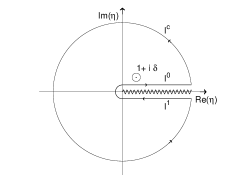
Figure 1: Contour used to evaluate $R_{\omega}^{0}$

Following the contour in the complex plane as shown in FIG. 1, we express the contour integral as

$$\oint d\eta f(\eta)=I^{0}+I^{1}+I^{c}=(2\pi i)~{}\mathrm{Res}[f(\eta)]_{|\eta=1+i\delta}~{},$$ (47)

where $\mathrm{Res}[f(\eta)]_{|\eta=1+i\delta}$ denotes the residue of the function $f(\eta)$ evaluated at the pole $\eta=(1+i\delta)$. Using the properties that $I^{c}=0$ and $I^{1}=-e^{2\pi\omega/a}~{}I^{0}$, non-transient part of the transition rate can be expressed as

$$R_{\omega}^{0}=I^{0}=\frac{-(2\pi i)\mathrm{Res}[f(\eta)]_{|\eta=1+i\delta}}{e^{2\pi\omega/a}-1}~{}.$$ (48)

The evaluated residue at the pole of the two-point function in Fock space

$$\mathrm{Res}[f(\eta)]_{|\eta=1+i\delta}=\frac{i\omega}{2\pi}~{},$$ (49)

leads the induced transition rate to become

$$R_{\omega}^{0}=\frac{\omega}{e^{2\pi\omega/a}-1}~{}.$$ (50)

In other words, the induced transition rate $R_{\omega}^{0}$ is precisely equal to the standard expression for mean energy per mode of a system in thermal equilibrium at the Unruh temperature $T=a/2\pi k_{B}$.

The transient part $\Delta R_{\omega}$ can be computed easily by considering reasonably large but finite time of observation as

$$\Delta R_{\omega}({\tau})\approx\frac{e^{-a\tau}}{\pi\left(1+\omega^{2}/a^{2}\right)}\left[a\cos(\omega\tau)-\omega\sin(\omega\tau)\right].$$ (51)

The transient terms decays out exponentially as the time of observation increases.

We summarize two key inputs that are required to arrive at the equation (50). Firstly, to ensure $I^{c}=0$ the function $f(\eta)$ should have sufficient fall-off as $\eta\to\infty$ so that Jordan’s lemma is applicable i.e. $\lim_{\eta\to\infty}|f(\eta)|=\lim_{\eta\to\infty}|G(\eta)/\eta|=0$. Secondly, in order to have a non-zero residue, the function $f(\eta)$ should have at least one pole within the region enclosed by the contour. It is evident from the equation (46), the short-distance singular nature of the Fock space two-point function is a key requirement to ensure non-vanishing residue. In other words, the pole of two-point function $G(\eta)$ at ($\eta-1)=i\delta$ plays the crucial role for the existence of the Unruh effect.

VIII Polymer quantization

In order to perform the so-called polymer quantization of scalar field, we follow the approach as suggested here Hossain et al. (2010) and was followed up later to study Unruh effect Hossain and Sardar (2016, 2015). In this approach, one quantizes the system of Fourier modes using polymer quantization instead of Schrödinger quantization as used in Fock space. As mentioned earlier, Polymer quantization or loop quantization is a quantization technique that is used in loop quantum gravity and it comes with a new dimension-full parameter say $l_{\star}$ along with Planck constant $\hbar$. In full quantum gravity, the parameter $l_{\star}$ would be analogous to Planck length.

The energy spectrum of the $\mathrm{k}-$th oscillator mode in polymer quantization are given by Hossain et al. (2010)

$$\frac{E_{\mathrm{k}}^{2n}}{|\mathrm{k}|}=\frac{1}{4g}+\frac{g}{2}~{}A_{n}(g)~{},~{}\frac{E_{\mathrm{k}}^{2n+1}}{|\mathrm{k}|}=\frac{1}{4g}+\frac{g}{2}B_{n+1}(g)~{},$$ (52)

where $n\geq 0$, $A_{n}$, $B_{n}$ are Mathieu characteristic value functions and $g=|\mathrm{k}|~{}l_{\star}$ is a dimension-less parameter. The energy eigenstates are $\psi_{2n}(v)=\mathrm{ce}_{n}(1/4g^{2},v)/\sqrt{\pi}$ and $\psi_{2n+1}(v)=\mathrm{se}_{n+1}(1/4g^{2},v)/\sqrt{\pi}$ where $v=\pi_{\mathrm{k}}\sqrt{l_{\star}}+\pi/2$. The functions $\mathrm{ce}_{n}$ and $\mathrm{se}_{n}$ are solutions to Mathieu equation. They are referred as elliptic cosine and sine functions respectively Abramowitz and Stegun (1964). In order to arrive at these $\pi$-periodic and $\pi$-antiperiodic states in $v$, superselection rules are invoked. This superselection leads to exact energy spectrum which in turns allows to study the system analytically. Besides, without imposition of superselection rules, certain key statistical notions for the system are known to become ill-defined Barbero G. et al. (2013).

For low-energy modes i.e. for small $g$, the energy spectrum (52) reduces to regular harmonic oscillator energy spectrum along with perturbative corrections

$$\frac{E_{\mathrm{k}}^{2n}}{|\mathrm{k}|}\approx\frac{E_{\mathrm{k}}^{2n+1}}{|\mathrm{k}|}\approx\left(n+\frac{1}{2}\right)+\mathcal{O}(g)~{}.$$ (53)

Therefore, polymer quantization leads to expected results for low-energy modes. However, we note that polymer energy spectrum has two-fold degeneracy as $g\to 0$ and it is lifted for finite values of $g$. The coefficients $c_{4n+3}=i\sqrt{l_{\star}}\int_{0}^{2\pi}\psi_{4n+3}\partial_{v}\psi_{0}dv$ are non-vanishing in polymer quantization for all $n=0,1,2,\ldots$, unlike in Fock quantization where only one $c_{n}$ is non-vanishing (38). Using asymptotic properties of Mathieu functions, we can approximate the energy gaps $\Delta E_{n}$ between the levels and coefficients $c_{4n+3}$ for low-energy modes or sub-Planckian modes (i.e. $g\ll 1$) as

$$\frac{\Delta E_{4n+3}}{|\mathrm{k}|}=(2n+1)-\frac{(4n+3)^{2}-1}{16}g+\mathcal{O}\left(g^{2}\right)~{},$$ (54)

for $n\geq 0$, and

$$c_{3}=\frac{i}{\sqrt{2|\mathrm{k}|}}\left[1+\mathcal{O}\left(g\right)\right]~{},~{}\frac{c_{4n+3}}{c_{3}}=\mathcal{O}\left(g^{n}\right),$$ (55)

for $n>0$. On the other hand, for high energy modes or super-Planckian modes (i.e. $g\gg 1$), we can approximate the energy gaps and coefficients $c_{4n+3}$ as

$$\frac{\Delta E_{4n+3}}{|\mathrm{k}|}=2(n+1)^{2}g+\mathcal{O}\left(\frac{1}{g^{3}}\right),$$ (56)

for $n\geq 0$, and

$$c_{3}=i\sqrt{\frac{g}{2|\mathrm{k}|}}\left[\frac{1}{4g^{2}}+\mathcal{O}\left(\frac{1}{g^{6}}\right)\right],\frac{c_{4n+3}}{c_{3}}=\mathcal{O}\left(\frac{1}{g^{2n}}\right),$$ (57)

for $n>0$. Therefore, we can approximate matrix element $D_{\mathrm{k}}(\Delta t)$ in polymer quantization as

$$D_{\mathrm{k}}^{poly}(\Delta t)\simeq|c_{3}|^{2}e^{-i\Delta E_{3}\Delta t}~{},$$ (58)

for both the cases.

VIII.1 Short-distance two-point function

As discussed earlier, the singular nature of the short-distance two-point function plays the key role in providing non-vanishing residue to the expression of induced transition rate (50) in Fock space. Therefore, in order to understand the effect of polymer quantization on the response function of Unruh-DeWitt detector it is crucial to determine the form of short-distance two-point function (i.e. near $(\eta-1)=0$) in polymer quantization.

Given $\eta\to 1$ implies $|\Delta\mathbf{x}|\to 0$, we may express the two-point function $G(x,x^{\prime})=G_{+}-G_{-}$, as a series of the form

$$G=\sum_{m=1}^{\infty}\frac{(-2i|\Delta\mathbf{x}|)^{m-1}}{2\pi^{2}m!}\int_{0}^{\infty}dk~{}k^{m+1}D_{k}(\Delta t)e^{i\mathrm{k}|\Delta\mathbf{x}|}~{},$$ (59)

where we have used the identity $e^{-x}=e^{x}\sum_{m=0}^{\infty}(-2x)^{m}/m!$.

In Fock quantization, the matrix element has exact expression $D_{\mathrm{k}}(\Delta t)=(1/2|\mathrm{k}|)e^{-i|\mathrm{k}|\Delta t}$ whereas in polymer quantization we can approximate it as $D_{\mathrm{k}}(\Delta t)\simeq|c_{3}|^{2}e^{-i\Delta E_{3}\Delta t}$. In other words, we can represent the matrix element for both the cases in a general form $D_{\mathrm{k}}(\Delta t)=|c_{k}|^{2}e^{-i\Delta E_{k}\Delta t}$. Further, in the domain where $(\eta-1)$ is very small, the temporal and the spatial separations satisfies $\Delta t\gg|\Delta\mathbf{x}|$ and $\Delta E_{3}/k$ is at least $\mathcal{O}(1)$ or higher for all modes. So by defining a new variable $u=\Delta E_{k}(\eta-1)/a$ and keeping only the leading term, we may approximate the two-point function (59) as

$$G(\eta)=\int_{0}^{\infty}du~{}h(u,\eta)~{}e^{-iu}+\mathcal{O}(\eta-1)~{}.$$ (60)

where

$$h(u,\eta)=\frac{k^{2}|c_{k}|^{2}}{2\pi^{2}}\frac{dk}{du}~{}.$$ (61)

Unlike in Fock quantization, the expression for $|c_{k}|^{2}$ and $\Delta E_{k}$ are different for sub-Planckian and super-Planckian modes in polymer quantization due to the presence of the scale $l_{\star}$. Therefore, here we consider the sub-Planckian and super-Planckian contributions to the two-point function separately as

$$G(\eta)=G_{sub}(\eta)+G_{super}(\eta).$$ (62)

The sub-Planckian contributions to the two-point function, is defined as

$$G_{sub}(\eta)\equiv\int_{0}^{u_{0}}du~{}h(u,\eta)~{}e^{-iu}+\mathcal{O}(\eta-1)~{},$$ (63)

where $u_{0}=\Delta E_{k_{0}}(\eta-1)/a$ and $k_{0}$ is some pivotal value of the wave-vector chosen such that $k_{0}l_{\star}$ is $\mathcal{O}(1)$. The limit $\eta\to 1$ implies $u_{0}\to 0$ which in turns leads $G_{sub}(\eta)\to\mathcal{O}(l_{\star}^{-2})$. On the other hand, the super-Planckian contributions to the two-point function, defined by

$$G_{super}(\eta)=\int_{u_{0}}^{\infty}du~{}h(u,\eta)~{}e^{-iu}~{},$$ (64)

are expected to dictate the short-distance ($\eta\to 1$) behaviour of the two-point function. Using the asymptotic expressions (56) and (57), one can compute the expression for $h(u,\eta)$ for polymer quantization as

$$h^{poly}(u,\eta)=\frac{u^{-3/2}}{64\pi^{2}l_{\star}^{2}}\sqrt{\frac{\eta-1}{2al_{\star}}}\left[1+\mathcal{O}(\eta-1)\right]~{}.$$ (65)

Therefore, the short-distance two-point function with non-perturbative modifications from polymer quantization can be expressed as

$$G^{poly}(\eta)=-\frac{(1+i)}{64\pi l_{\star}^{2}}\sqrt{\frac{\eta-1}{\pi al_{\star}}}\left[1+\mathcal{O}(\eta-1)\right]+\mathcal{O}(l_{\star}^{-2})~{},$$ (66)

where we have used analytic continuation to evaluate the integral as $\int_{0}^{\infty}du~{}u^{-3/2}e^{-iu}=-\sqrt{2\pi}(1+i)$.

We note here that the short-distance two-point function (66) instead of diverging, it reaches a maximum value of $\mathcal{O}(l_{\star}^{-2})$. This bounded from above behaviour of the two-point function is analogous to the behaviour of the spectrum of inverse scale factor operator as well as the effective Hubble parameter in loop quantum cosmology (LQC) Bojowald (2001a, b); Ashtekar et al. (2006a, b). Both of these can be associated with some inverse powers of the distance similar to the two-point function. In LQC, this crucial behaviour plays a key role in resolution of Big Bang singularity. However unlike in LQC, here we have applied polymer quantization only for scalar matter field rather than for the geometry.

We may verify that the equation (64) also reproduces the result of Fock quantization up to $\mathcal{O}(\eta-1)$ term as

$$G(\eta)=-\frac{a^{2}}{4\pi^{2}(\eta-1-i\delta)^{2}}\left[1+\mathcal{O}(\eta-1)\right]~{}.$$ (67)

Here we have used the Fock space expression $h(u,\eta)=\left(a/2\pi(\eta-1)\right)^{2}u$ that follows from the equation (38).

VIII.2 Detector response along Rindler trajectory

We note that unlike in Fock quantization, two-point function (66) does not have any pole as $\eta\to 1$. Therefore, the corresponding residue $\mathrm{Res}[f(\eta)]_{|\eta=1+i\delta}$ vanishes in polymer quantization. This in turns, leads non-transient part of the induced transition rate (48) to vanish i.e.

$$R_{\omega}^{0}=0~{}.$$ (68)

Thus, from the response of the Unruh-DeWitt detector which interacts with polymer quantized scalar field, one would conclude that Unruh effect is not present in polymer quantization. We should mention here that the large-distance two-point function including polymer corrections was computed in Hossain and Sardar (2015) and it may be checked that Jordan’s lemma continues to be applicable even including polymer corrections.

As earlier, we may approximate the transient part of the transition rate by considering a reasonably large but finite observation time $\tau$. In particular, in the domain of perturbation where $(al_{\star})\ll 1$ and $e^{a\tau}\gg 1$, the transient part is

$$\Delta R_{\omega}({\tau})\approx\frac{e^{-a\tau}[1+\mathcal{O}(al_{\star})]}{\pi\left(1+\omega^{2}/a^{2}\right)}\left[a\cos(\omega\tau)-\omega\sin(\omega\tau)\right].$$ (69)

Clearly, the transient part of the induced transition rate decays exponentially in proper time $\tau$, similar to the results of Fock quantization. We should mention here that the polymer quantization is known to cause a violation of Lorentz invariance due to the presence of the length scale $l_{\star}$. As one of the consequences, it is shown in Husain and Louko (2016); Kajuri (2016) that polymer vacuum state is not strictly invariant under the boost. Therefore, the specific nature of the transient terms as studied here are effectively tied to the observer in polymer quantization.

IX Discussions

In summary, we have studied the properties of response function of an Unruh-DeWitt detector which moves along a Rindler trajectory and interacts weakly to a polymer quantized massless scalar field. Through a detailed calculation we have shown that unlike in Fock quantization, there are only transient terms present in the induced transition rate of the detector. In Fock quantization, the induced transition rate of the detector contains also a non-transient term which is proportional to Planck distribution. This property of the induced transition rate signifies the existence of Unruh effect in Fock quantization. In polymer quantization of scalar field, however, the non-transient term is absent. Therefore, an Unruh-DeWitt detector would not perceive a flux of thermal particles along an uniformly accelerating trajectory in polymer quantization. The result as shown here provides an alternative evidence for the earlier reported results by the authors where it is shown using method of Bogoliubov transformation Hossain and Sardar (2016) as well as using Kubo-Martin-Schwinger (KMS) condition Hossain and Sardar (2015) that Unruh effect is absent in polymer quantization.

We note the key ingredients that led to the main result of this paper. As evident from the equation (48), the induced transition rate of an Unruh-DeWitt detector along a Rindler trajectory is quite generically proportional to the Planck distribution formula (i.e. $\propto(e^{2\pi\omega/a}-1)^{-1}$). However, the proportionality constant contains the residue of the two-point function evaluated at its pole. Therefore, the short-distance singular nature of the Fock space two-point function is a key input to ensure the non-vanishing residue which in turns plays the crucial role for the existence of Unruh effect. On the other hand, it is widely expected that the short distance behaviour of the two-point function would receive significant modifications from possible Planck-scale physics. In this paper, we have shown that this expectation is indeed borne out in polymer quantization where the short-distance two-point function receives non-perturbative modifications. In particular, the short-distance singular two-point function is replaced by a regular function which has no divergence in short-distance.

Finally, we may recall that several experiments have been proposed to detect possible signatures of Unruh effect in laboratory Schutzhold et al. (2006, 2008); Aspachs et al. (2010). Therefore, the result as shown here using response function of an Unruh-DeWitt detector and also shown earlier using methods of Bogoliubov transformation Hossain and Sardar (2016) and Kubo-Martin-Schwinger (KMS) condition Hossain and Sardar (2015) where criticism raised in Rovelli (2014) was also addressed, clearly indicates that the experimental detection of Unruh effect can be used as a probe of possible Planck-scale physics. In particular, such a detection can be used to either verify or rule out a candidate Planck scale theory with a new dimension-full parameter, which affects quantization of matter fields as considered here. We conclude by acknowledging few similar recent results in the context of polymer quantization where it is shown that some high energy modifications can indeed lead to the alteration of certain low energy phenomena Husain and Louko (2016); Kajuri (2016). In particular, it is shown in Husain and Louko (2016); Kajuri (2016) that polymer vacuum state is not strictly invariant under the boost. Therefore, the specific nature of the transient terms as studied here are effectively tied to the observer in polymer quantization. However, the transient terms are shown to decay out exponentially. So the detector response after a reasonably long time, in the scale of $a^{-1}$, becomes essentially time independent. Clearly, the existence of Unruh effect needs to be understood from the properties of the non-transient part of the detector response as studied here.