Probabilistic Model to Treat Flexibility in Molecular Contacts

Abstract

Evaluating accessible conformational space is computationally expensive and thermal motions are partly neglected in computer models of molecular interactions. This produces error into the estimates of binding strength. We introduce a method for modelling interactions so that structural flexibility is inherently taken into account. It has a statistical model for 3D properties of nonlocal contacts and a physics based description of local interactions, based on mechanical torque. The form of the torque barrier is derived using a representation of the local electronic structure, which is presumed to improve transferability, compared to traditional force fields. The nonlocal contacts are more distant than 1-4 interactions and Target-atoms are represented by 3D probability densities. Probability mass quantifies strength of contact and is calculated as an overlap integral. Repulsion is described by negative probability density, allowing probability mass to be used as the descriptor of contact preference. As a result, we are able to transform the high-dimensional problem into a simpler evaluation of three-dimensional integrals. We outline how this scoring function gives a tool to study the enthalpy–entropy compensation and demonstrate the feasibility of our approach by evaluating numerical probability masses for chosen side chain to main chain contacts in a lysine dipeptide structure.

1 Introduction

A computationally affordable approach that would allow for chemically accurate simulation of interactions in large protein complexes in a given molecular environment, would be decisively useful for the study of biological systems. Namely, this would open up new avenues for theoretical analysis of biochemical processes and aid in the design of complex molecular components in bioscience research. Extensive molecular modeling at the molecular systems level is an emerging, multifaceted field and a manifestation of chemical physics applied to biology [1]. Molecular simulations are based on computational methods that describe molecular interactions and so regulate the virtual model of the studied system. There exist several methods that can be used to routinely calculate strengths of static interactions for any given complex of molecular structures, see e.g. refs[2, 3], but incorporating such factors as thermal motion and flexibility, that are required for the model to be considered realistic, has proven a significant challenge. These factors are of great importance in understanding, for example, the process of molecular complex formation [4] and for predicting relative protein conformations [5]. One specific example where the detailed understanding of the variability of also the local protein structure has an essential role, is given by the function of an ion channel [6]. We are developing a method to treat flexibility and thermal motion in macromolecular systems, including protein-ligand interactions. In this work we outline the basic principles of the approach and apply the method to a small structure (a lysine dipeptide), accessible at the present stage of implementability, see Discussion for details. The current difficulties of force fields, solving of which also our method is targeted for, are discussed in a somewhat different setting of nanostructures in, e.g., section 2.4 of ref [7].

The method presented here treats internal (local) molecular conformations in terms of classical mechanics, but for external (nonlocal) contacts incorporates a concept used in quantum theory formalism, namely the overlap integral for functions of position, see e.g. [8, pp. 154-156, 325-326]. Overlap probability mass quantifies here the strength of an interaction, and is defined directly based on 3D probability densities, instead of wave functions which do not appear in this approach. We therefore try to approximate the information that is assumed, for example, a quantum chemistry description would produce. At present, this is done through experimental coordinate data and prior chemical knowledge. Quantum chemistry results are used as reference, though not necessarily directly. Namely, questions concerning the role of interactions involving varying electron densities, like dispersion [9], are at least in the present model considered further than 1-4 interactions and therefore implicit in the molecular fragment classification. In general, the fragment classification is central to how quantitative this method is, or can be.

Strain determines internal preferences in the molecular structure and is in our approach described with the classical mechanical moment of force $\bar{r}\times\bar{F}$, i.e., the cross product of a position vector with a force vector. It has the unit newton meters (Nm), and quantifies here how strongly an internally rotating structure is influenced by the charge distributions present at each end of a rotatable bond, so that the system is forced to move towards an equilibrium conformation. This approach was chosen to treat the flexible molecule as a mechanical system composed of levers and pivot points, not masses in space experiencing potentials. Namely, torque is considered as a natural quantity for describing a covalent structure. Rotations about single bonds are the primary form of motion realizing the structural flexibility considered in this work. Rotational barriers over full rotations around rotatable bonds are calculated based on the moment of force. Adjustable average bond angles and lengths are used, though bending and stretching of bonds could be taken into account through the same scheme, by making the parameter bond angles and lengths depend on the angle of rotation. Nevertheless, at least with respect to the relevant case here, a substituted hydrocarbon straight chain segment, an average constant bond angle seems reasonable, because of bond angle stabilizing electrostatic interactions over adjacent rotatable bonds. The main goal of this paper is to describe a novel approach for modeling molecular structure and interactions, and to demonstrate how this probabilistic method is used to obtain chemically relevant and commensurate numerical information.

The partitioning of model components differs here from a typical force field [11, 2, 10, 7], in that the energy landscape of internal rotations for a molecule is analytically further defined. In practical terms, the dihedral part of a molecular mechanics force field has a partially predefined functional form, with parameters whose values are derived from fitting either to experimental data or to quantum chemistry calculations. In contrast, the form of the internal torque is here derived using a representation of electronic structure, i.e., elementary properties of the electronic structure is the source of parameters. This approach is expected to improve the transferability [12, 3] of the energy function, as compared to traditional force fields. Another important feature is that the structural flexibility [4, 14, 13] allowed by the degrees of freedom and utilized by thermal energy, is captured in one theoretical object, a three dimensional probability density. Using these densities together with the overlap integral method, makes it possible to simultaneously describe noncovalent interaction strength and restrictions to the freedom of motion.

The Method section describes advances made in this study to an existing model framework from our previous work [16, 15]. These in turn recast the founding work by Rantanen et al. [17]. In section Results, we show how the method has been refined, especially its ability to capture the fundamentally important molecular flexibility and the way this is incorporated in the contact preference calculations. We also describe how repulsion can be treated as negative probability and outline enthalpy–entropy compensation as a result of the spatial properties of interactions. Then, we present numerical results from applying the method to a test structure. Finally, in the Discussion, we consider potential ways of further improving the model.

2 The Method

This is a molecular fragment based method. It means here three-atom fragments (each belonging to a class in a chemical classification, see e.g. [16]) that are selected from the studied molecules. A reference frame is attached to each chosen fragment, in order to model its noncovalent contacts in the system. The reference frame, together with pre-determined 3D probability densitities, called contact preference densities, allow for both distance and direction dependent analysis of the interactions with a chosen molecular environment. Final step in estimating the strength of a contact is evaluating an overlap integral. The integrand is derived from the contact preference density and a Target-atom distribution, where the latter has also been modelled as a 3D probability density. In determining the distribution of the Target-atoms, internal preferences of the interacting molecular structures and a thermal energy level (or a distribution of levels) are required. The internal preferences consist of the torque based strain (local) together with possible intramolecular contacts (nonlocal).

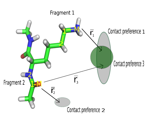
Figure 1: Molecular fragments and their contact preferences. In figure shown the structure used as a test structure (lysine dipeptide, see text for details). Calculations require three-atom fragments (M-1-2, yellow), for which 3D probabilistic contact preferences have been determined. The latter shown schematically (filled ellipses) for two fragments, with position vectors from fragment to a point inside preference density with corresponding indeces (1,2 or 3).

2.1 Reference frame and molecular fragment

Orienting a molecular fragment in three dimensional space requires three atoms, called here M, 1 and 2. This is depicted in Figure 1 using the end group of lysine side chain and a carbonyl group from the main chain as examples. The former belongs to the fragment class for Primary amine nitrogens bonded to an aliphatic structure (class f26 in [16]) and the latter to the class for Amide group oxygens bonded to a non-aromatic structure (class f26 in [16]). In Figure 1, the Main-atoms M are NZ and O, using Protein Data Bank atom names, and the two other atoms (1 and 2) are, correspondingly, the next two carbons in the side-chain and the other two atoms of the amide group (C and N ), as shown. The bonds in the lysine side chain being rotatable, NZ can obtain positions from a complicated spatial distribution. A convention used in this work for calculations, is that a fragments rotatable bond is always the bond between Main-atom M and atom 1, the fragment realization in the studied structure is changed accordingly.

A representation of the local electronic structure is required for describing the internal local strain in a molecular structure. The representation used in this work consists of point charges on atoms and bonds, i.e., in addition to a standard partial charges scheme, also bonds between atoms are assigned separate charges. This approach is used because molecular strain is produced in this model by torque, which depends on distance (along a covalent bond) from the pivot point (an atom). Also, the distance between atoms that are directly bonded to two adjacent atoms, like the ends of a rotatable bond, is not large compared to dimensions of a bond-atom charge distribution, so that the validity of a multipole expansion is not obvious for the 1-4 interaction.

The immediate local structure, centered around a rotatable bond, is schematically illustrated in Figure 2. There the Main-atom (M) and atom 1 would be connected by the rotatable bond $a$, and atom 2 could be the one having the parameter charge $q_{1}$, i.e., one bond away from the axis of rotation, on the $\beta$ angle side of the axis bond.

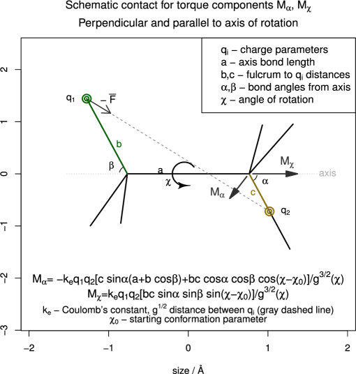
Figure 2: Torque parameters for electrostatic interaction over a rotatable bond. Potential energy is replaced in this method by two components of torque, to an angle of rotation unit vector direction ($M_{\alpha}$) and to axis of rotation direction ($M_{\chi}$). The total amount of torque causing strain in the structure is a sum of individual terms shown in the lower part of the graphics. These terms correspond to parameter charge pairs in covalent bonds ($q_{2}$) and on atoms ($q_{1}$), including atom–atom, atom–bond and bond–bond interactions. The depicted direction of force vector $-\bar{F}$ corresponds to opposite $q_{1}$ and $q_{2}$ charges. $M_{\alpha}$ has one of infinitely many directions perpendicular to the axis of rotation.

2.2 Torque model of internal strain

The rotation barrier structure is in the following determined for a single rotatable bond contribution to the background internal energy state (strain without nonlocal contacts). It is calculated as torque due to force couples of oscillating classical electrostatic forces produced by parameter charges. As stated, these charges are in bonds and on atoms in the vicinity of both ends of the rotatable bond, but not as part of it, see Figure 2. The interaction can be described using Coulomb’s inverse square law between the individual charges [18, pp. 27-37], which gives a realistic force estimate (in vacuum), provided that the point charge distribution is representative of the interacting spatial charge distributions.

In addition to the mechanical suitableness and alleged better transferability, shortly discussed in Introduction, another useful aspect is that because the existence of a well defined potential for the hindered rotation is not presumed, path-dependence of internal rotations could in principle be studied. Namely, forces depending on variables disturbing the definition of a potential, like velocity ($\bar{F}(\bar{r},\dot{\bar{r}})$), can be used to model suspected internal (to structure) friction and dispersion in the local component of the method.

Torque equations

In order to model the energy states during internal rotation, the combined torque produced by two force components at each end of the rotatable bond is used. One component is towards the direction of bond bending and the other towards the direction of rotation. The corresponding moments of force, $M_{\alpha}$ and $M_{\chi}$, are then defined with respect to a pivot point (an atom at one end of a rotatable bond) and the axis of rotation (the z-axis as defined in this work), see schematic Figure 2 for details. The primary factor expressing variation in internal angular preference is the change in the sum of the net values of these torque components, separately added over all parameter charge interactions. Using bond and angle naming convention shown in Figure 2, equation for the (axial) vector torque components is

$$\bar{M}=[\bar{c}\times\bar{F},\bar{b}\times(-\bar{F})]$$ (1)

where a half of the force couple is

$$\bar{F}=\bar{F}_{\rho}+\bar{F}_{\alpha}+\bar{F}_{\chi}=F_{\rho}\bar{u}_{\rho}+F_{\alpha}\bar{u}_{\alpha}+F_{\chi}\bar{u}_{\chi}=-F^{(b)}_{\rho}\bar{u}^{(b)}_{\rho}-F^{(b)}_{\alpha}\bar{u}^{(b)}_{\alpha}-F^{(b)}_{\chi}\bar{u}^{(b)}_{\chi}$$ (2)

and $\bar{u}_{\rho}$ is along a rotating bond, $b$ and $c$ in Figure 2. Vector $\bar{u}_{\chi}$ is the unit tangent vector of the $\chi$-related rotation arch tracked by a parameter charge, $q_{i}$ in Figure 2, and $\bar{u}_{\alpha}$ is the same for bond bending, parameterized by angles $\alpha$ and $\beta$. The superscript $b$ refers to the components at that end of the rotatable bond with parameters $b$ and $\beta$. The force components have the form given in Table 2.2, where the multiplier $k(\chi)$, that contains the angle of rotation dependent squared distance (in square brackets), has the form

$$k_{i}(\chi)= k_{e}q_{1}q_{2}[a_{i}^{2}+b_{i}^{2}+c_{i}^{2}+2a_{i}c_{i}\cos(\alpha_{i})+2a_{i}b_{i}\cos(\beta_{i})+2b_{i}c_{i}\cos(\alpha_{i})\cos(\beta_{i})-$$

$$2b_{i}c_{i}\sin(\alpha_{i})\sin(\beta_{i})\cos(\chi-\chi^{(i)}_{0})]^{-\frac{3}{2}}$$ (3)

The definitions given in Figure 2 for the structural parameters (${a,b,c,\alpha,\beta,\chi_{0}}$) are in respective order: axis bond length, two distances from pivot point, two bond angles and an orientation of one of the bonds ($\chi_{0}$ is not rotated, but kept fixed during rotatable bond specific computations), and $k_{e}$ is Coulomb’s constant.

Force components needed for calculating torque caused by rotation about a bond. Component Definition Functional form $F_{\chi}$ $\bar{F}\cdot\bar{u}_{\chi}$ $k(\chi)b\sin\beta\sin(\chi-\chi_{0})$ $F^{(b)}_{\chi}$ $\bar{F}\cdot\bar{u}^{(b)}_{\chi}$ $k(\chi)c\sin\alpha\sin(\chi-\chi_{0})$ $F_{\alpha}$ $\bar{F}\cdot\bar{u}_{\alpha}$ $-k(\chi)(\sin\alpha(a+b\cos\beta)+b\cos\alpha\cos\beta\cos(\chi-\chi_{0}))$ $F^{(b)}_{\alpha}$ $\bar{F}\cdot\bar{u}^{(b)}_{\alpha}$ $k(\chi)(\sin\beta(a+c\cos\alpha)+c\sin\alpha\cos\beta\cos(\chi-\chi_{0}))$ Superscript $b$ referes to definitions of the force components at the other end of the $\chi$-rotatable bond. Factor $k$ includes the Coulomb constant and the distance between the interacting parameter charges $q_{1}$ and $q_{2}$. Parameters $(a,b,c,\alpha,\beta)$ are defined in Figure 2 and $\chi_{0}$ is a fixed angle of rotation value.

The force components to the direction of the rotating bond, $\bar{F}_{\rho}$ and $\bar{F}^{(b)}_{\rho}$, do not contribute to the torque, because they are parallel to the respective position vectors $\bar{c}$ and $\bar{b}$. By using the force component definitions given in Table 2.2, the torque $\bar{M}$ in Equation 1 is given as

$$\bar{M} =[cF_{\alpha}(\bar{u}_{\rho}\times\bar{u}_{\alpha}),cF_{\chi}(\bar{u}_{\rho}\times\bar{u}_{\chi}),bF^{(b)}_{\alpha}(\bar{u}^{(b)}_{\rho}\times\bar{u}^{(b)}_{\alpha}),bF^{(b)}_{\chi}(\bar{u}^{(b)}_{\rho}\times\bar{u}^{(b)}_{\chi})]$$

$$=[cF_{\chi}(-\bar{u}_{\alpha}),cF_{\alpha}\bar{u}_{\chi},bF^{(b)}_{\chi}(-\bar{u}^{(b)}_{\alpha}),bF^{(b)}_{\alpha}\bar{u}^{(b)}_{\chi}]$$ (4)

In Equation 4, rules for calculating cross products ($\times$) are used to obtain the expressions on the second line. The moment of force $M_{\chi}$ can be extracted from Equation 4 by representing the bond bending angle unit vector as a sum of components: $\bar{u}_{\alpha}=\sin\gamma\bar{u}_{R}+\cos\gamma\bar{k}$, $\gamma=\alpha,\beta$, where $\bar{k}$ is the unit vector to the direction of the axis of rotation (the z-axis in this case). Taking into account all simultaneous contacts $i$ and reordering the terms to group those that are with respect to the end atoms and those that are with respect to the axis of rotation, the magnitude for the moment of force can be expressed as

$$M =|\sum_{i=1}^{N}M^{(i)}_{\alpha}|+|\sum_{i=1}^{N}M_{\alpha}^{(b,i)}|+|\sum_{i=1}^{N}M^{(i)}_{\chi}|+|\sum_{i=1}^{N}M^{(b,i)}_{\chi}|$$

$$=|\sum_{i=1}^{N}c_{i}F^{(i)}_{\alpha}|+|\sum_{i=1}^{N}b_{i}F^{(b,i)}_{\alpha}|+|\sum_{i=1}^{N}c_{i}F^{(i)}_{\chi}\sin\alpha_{i}|+|-\sum_{i=1}^{N}b_{i}F^{(b,i)}_{\chi}\sin\beta_{i}|$$

$$=|-\sum_{i=1}^{N}k_{i}(\chi)(c_{i}\sin\alpha_{i}(a_{i}+b_{i}\cos\beta_{i})+b_{i}c_{i}\cos\alpha_{i}\sin\beta_{i}\cos(\chi-\chi^{(i)}_{0}))|\>+$$

$$\,+|\sum_{i=1}^{N}k_{i}(\chi)(b_{i}\sin\beta_{i}(a_{i}+c_{i}\cos\alpha_{i})+b_{i}c_{i}\sin\alpha_{i}\cos\beta_{i}\cos(\chi-\chi^{(i)}_{0}))|\>+$$

$$+2\,|\sum_{i=1}^{N}k_{i}(\chi)b_{i}c_{i}\sin\alpha_{i}\sin\beta_{i}\sin(\chi-\chi^{(i)}_{0})|$$ (5)

In Equation 5, the first two torque terms correspond to bond bending strain $M_{\alpha}$, the third and fourth to torsional strain $M_{\chi}$. Subscript $b$ refers to that end of the rotatable bond which is parametrized with angle $\beta$ and length $b$, as given in Figure 2. Vertical bars in Equation 5 mark an absolute value and $k(\chi)$ is given by Equation 3. The bond angles $\alpha$ or $\beta$ ($\pi-\beta$), between a rotatable bond and a rotating ($\alpha$) or a reference bond ($\pi-\beta$) correspond, as defined here, to the polar angle of the spherical polar coordinates in the fragment reference frame.

The x-axis of the fragment reference frame determines the zero point for $\chi$ and $\chi_{0}$ in Equations 3 and 5. Parameter $\chi_{0}^{(i)}$ (i=1,2,3) can have, for example, the values [$\frac{\pi}{3}$,$\pi$,$\frac{5\pi}{3}$]. The barriers of Equation 5 could be calculated using continuous charge distributions, but a simple point charge model is regarded as sufficiently representative of the distribution for our purposes here.

In practice, there are four independent force couples for each bond pair (four bond charge and atom charge over-bond combinations, $q_{1,3}$ — $q_{2,4}$) and six or nine rotating covalent bond combinations. This means for barrier to rotation calculations, that one uses a sum of 24 or 36 (parameter N) terms of the form given in Equation 5, with angle of rotation $\chi$ dependent forces and position vectors. Note that in this work we use in practice only the bond bending torque $M_{\alpha}$, which choise is discussed later in this section.

There is no straightforward connection between the functional forms of $M$ and a force field, as given in [2, 7], because the parameterizations are different, for example, $M$ combines both dihedral and bond bending angles in one function.

2.3 Overlap method and interaction strength

2.3.1 Position distribution

As described in this section, treatment of molecular contacts requires in our model, starting with a system of initial molecular structures, a distribution of allowed positions $\bar{r}_{\text{ref}}$. These are either positions of the atoms that are considered to interact with a studied fragment, or positions of interest with respect to a molecular fragment. The former is the so called Target-atom (NZ in Figure 8) and the latter needed in formulating the overlap integral, e.g., when the noncovalent bond is mediated with a small molecule like water. Mediated contacts were calculated in this way in ref [15]. It should be mentioned, that the roles (fragment side and Target side) can be reversed and naturally the same quantitative results should be obtained. The position distribution is here generated by rotations about relevant rotatable bonds in a structure, see Equations 6 and 8 for details of the procedure used.

Positions found during a systematic mapping on a conformational space are chosen for further use based on level of torque in the related structural conformations. Form of the torque is a sum of the single-bond contributions given by Equation 5. All conformations accessible on a thermal energy level are equally probable. The non-uniform distribution around a mean angle value in a rotamer library, see [19] for a continuous library, appears when a distribution of levels is used. A single level can represent the mean thermal energy for one or several degrees of freedom, in which case the generated position distribution is an average, lacking more rare motions of larger amplitude but also the accrual, corresponding to small angular deviations from an equilibrium position (minimum torque).

Conformation generation

The relevant unit here is an amino acid residue, or more precisely, a lysine side chain. The 3D point distribution was generated from an initial Target-atom position $\bar{r}_{M}^{(0),(\text{ref})}$ with the following procedure:

$$\bar{r}^{(1->N)}_{\text{ref}}(\chi_{1},...,\chi_{n-2},\phi,\psi)=\sum\limits^{N}_{i=1}(\prod\limits_{j=N}^{i}R_{j}\,[\bar{r}_{M}^{(i-1),(\text{ref})}-\bar{r}_{M}^{(i),(\text{ref})}])+\bar{r}_{M}^{(N),(\text{ref})}$$ (6)

In Equation 6, the subscript $M$ refers to the Main-atom of a molecular fragment $f(i)$. The respective position vector together with rotations $R_{i}$ are determined separately for each step. The rotations can all be with a different rotatable bond on the axis of rotation, all about the same bond, or something in between. Typically a fragment is involved more than once in the procedure (then at least two fragment definitions $f(i)$ and $f(j)$ are the same, i.e., defined by the same atom identifiers like NZ). Vector $\bar{r}^{(1->N)}_{\text{ref}}$ gives a single point produced by an arbitrary sequence of $N$ discrete rotation steps. The position of the reference point (starting from $\bar{r}_{M}^{(0),(\text{ref})}$) is tracked by ($n-2$) side chain angles of rotation and the overall conformation of the residue is additionally affected through two main chain angles of rotation.

In separating the main chain (mc) and side chain (sc) angles we presume that internal preferences on mc-side of $C_{\alpha}$ and on sc-side of $C_{\alpha}$ do not affect each other. This approximation is considered to give sufficient accuracy for our purposes here, though further development of the model will include mc torque parameters and a treatment of branch points. The dihedral angle indexing (1,…,n-2) in Equation 6 starts from the rotatable bond closest to the side chain terminal group, which is a convention to point out the order of varying the angles that is used here for a systematic coverage of conformational space.

Vector term $\bar{r}_{M}^{(N),(\text{ref})}$ is the Main-atom position of the last fragment used. The starting position vector $\bar{r}_{M}^{(0),(\text{ref})}$ that appears in the first term of the sum in Equation 6, has also a more explicit definition that is given by Equation 8. The 3x3 rotation matrices $R_{i}$ combine orientations of the rotatable bond containing molecular fragment $f(i)$, with respect to the reference or base fragment frame (subscript ref), and a rotation in frame $f(i)$:

$$R_{i}(\Delta\chi_{i})=ROT_{(\text{ref}->M(i))}ROT_{\Delta\chi_{i}}ROT_{(M(i)->\text{ref})}$$ (7)

$\Delta\chi_{i}$ is the angular interval determining the rotation step in $f(i)$. Subscript $i$ indexes consecutive rotations. Position generation in Equation 6 includes visiting residues base fragment every time the rotatable bond changes, because the intermediate positions with respect to the base fragment are collected. An example set of side chain positions are represented in Figure 7 by the blue patch-like clouds, which are a plotted 3D kernel density estimate, Equation 23, of the generated Target-atom positions.

2.3.2 Interaction model

In the statistical model of either a Target-atom or a reference point (with respect to a fragment), information about the distribution is captured in a 3D probability density $f(\bar{r})$. The vector variable $\bar{r}$ can, as an example, be related to the starting position $\bar{r}_{M}^{(0),(\text{ref})}$ of a sequence of generated (Target-atom or reference point) positions, see Equation 6, through

$$\bar{r}_{k}=ROT_{(\text{ref}->M(k))}\,\bar{r}+\bar{r}_{M(k)},\>\bar{r}_{k}=\bar{r}_{M}^{(0),(\text{ref})}$$ (8)

Vector $\bar{r}_{k}$ in Equation 8, points to a chosen position with respect to the residues base fragment (e.g., $C_{\beta}$-$C_{\alpha}$-$C$ in lysine), subscript ref. In case $\bar{r}_{k}$ is the $k^{\text{th}}$ fragment Main-atom position vector $\bar{r}_{M(k)}$, the length of $\bar{r}$ equals zero. When the fragment, typically chosen for exploring a noncovalent contact, is the same as the residues base fragment, then $ROT_{(M(k)->\text{ref})}$ is the indentity matrix and $\bar{r}_{k}=\bar{r}+\bar{r}_{M}$. Combining these two cases gives origo, the base fragment Main-atom position.
This conformational space managing scheme is primarily for one structural complex of the size involving, e.g., a few residues and ligands as flexible entities at a time. Incorporating larger scale structural motions is left for further study, as planned in Discussion.

Overlap probability mass

Given a contact preference probability density for a fragment $f_{p}$ and a Target-atom density $g_{t}$, a quantitative measure for the strength of the contact is calculated as an overlap integral

$$OL=\int_{\mathbb{R}^{3}}f_{p}^{\frac{1}{2}}(\bar{r}(\bar{r}_{k}))\,g_{t}^{\frac{1}{2}}(\bar{r})\,\mathrm{d}^{3}\bar{r}$$ (9)

There $\bar{r}_{k}$ (as in Equation 8) is defined with respect to the reference frame of the studied fragment, as positioned and oriented in 3D space. The second equality in Equation 8 means now that the present conformation, with corresponding position and orientation of the $k^{\text{th}}$ fragment, can be a starting structure for next structural manipulations. That is, probability density $f_{p}$ is defined relative to the frame of a studied fragment, but as seen from the base frame, where the target distribution $g_{t}$ is defined, or modelled.

The integral in Equation 9 is in principle over all space and the integrand is a preference–target overlap probability density. Depending on the definitions of $g_{t}$ and $\bar{r}_{k}$, the integrand corresponds either to a direct contact between structures (molecular fragment and a Target-atom or, in the future, two molecular fragments) or a bond mediated by at least one entity, like a water molecule or a metal ion. The value of the overlap integral includes the effect of structural flexibility, through the spatial form of the integrand. This is demonstrated in relation to the enthalpy-entropy compensation here in the corresponding section.

Determined by the plausible interactions, the overlap integral can contain $n>0$ preference densities. The generic equation with a target density $g_{t}$ is

$$OL_{\text{gen}}=\int_{\mathbb{R}^{3}}\sum\limits_{m=1}^{n}C_{m}\,f_{p,m}^{\frac{1}{2}}g_{t}^{\frac{1}{2}}\mathrm{d}^{3}\bar{r}$$ (10)

which is, as Equation 9, unitless in the sense that the outcome has dimensions of probability mass. The constant $C_{m}$ is introduced and has the meaning of an a priori chemical or physical information on the relative non-directional preference of the interaction. For example, a distance and electronegativity based set of these prior weights was defined and used in our earlier work [16]. This scheme can be developed further, so that the individual weights express physical relations between contacts, which makes the overlap probabilities comparable, i.e., independent of the complex and fragment classification. Next we introduce a probabilistic way to treat the unfavorable contacts.

Negative probabilities as repulsion

Contact preference densities $f_{p}$ in Equations 9 and 10 model attractive nonlocal interactions. This follows from the molecular fragment classification and distance criteria imposed while collecting the training data (e.g., $\leq$ 3.3 $\AA$ for a polar contact and $\leq$ 3.7 $\AA$ for alleged dispersion [16]). It should be mentioned that, though the interacting fragments and Target-atoms are not free to move in a complex structural setting, the distance and direction preferences are considered representative of the realized attractive interactions in a large sample of observed structures. Modelled repulsion needs to be added when structures and complexes are generated virtually, not observed experimentally.
More precicely, after that conformations adhering only to internal constraints (i.e., torque) have been generated to study interactions, contacts to the molecular environment are taken into account separately. Starting from a set of molecular conformations that are internally, or locally, preferred and then incorporating the set of conformations in a complex, requires modeling repulsive external interactions in addition to the attractive ones. Repulsion is in this framework described as negative probability density. This approach is chosen to have probability as the one common measure for preference.

Incorporating negative probabilities

Negative probability density that overlaps with positive, lowers the probability mass calculated for a contact. When the effect of repulsive components is surmounted by positive probability mass in the contact overall, formation of the complex can be considered as possibly preferred. Then, in case the probability mass of the initial state is lower than in the suggested complex, the formation is taken as preferred. In terms of energy balance, negative overlap probability density (OPD) means positive total energy $E$, whereas positive OPD corresponds to negative $E$. The case in between these two, when there is no OPD, describes $E=0$ and follows from no or only negligible interaction between the structural components.

The formal overlap calculation with, repulsion incorporating, contact preference probability density $f_{p,\pm}$ and target atom density $g_{t}$ is given here by the equation

$$OL =\int_{\mathbb{R}^{3}}f_{p,\pm}^{\frac{1}{2}}g_{t}^{\frac{1}{2}}\mathrm{d}^{3}\bar{r}=\int_{\mathbb{R}^{3}}(\sqrt{f_{p,+}}+i\sqrt{f_{p,-}})\,\sqrt{g_{t}}\,\mathrm{d}^{3}\bar{r}=$$ (11)

$$=\int_{\mathbb{R}^{3}}(\sqrt{|f_{p,+}|}-\sqrt{|f_{p,-}|})\,\sqrt{g_{t}}\,\mathrm{d}^{3}\bar{r}=\int_{\mathbb{R}^{3}}(\sqrt{|f_{p,+}||g_{t}|}-\sqrt{|f_{p,-}||g_{t}|})\mathrm{d}^{3}\,\bar{r}$$

Subscript $+$ refers to a positive and $-$ to a negative probability density. Vertical bars again mark absolute values. The functional form of the integrand follows from that the negative and positive parts effectively vanish where the other one is nonzero. The negative part is placed in an imaginary component, so that before taking the absolute values they are not defined in the same probability space and are in this way represented as separate. The first term of the final integrand in the second line of Equation 11 is the positive probability of the fragment–target interaction and the second term, as it is negative, lowers the value of the overlap probability mass $OL$. Normalization of the combined preference density $f_{p,\pm}$ in Equation 11 is componentwise.

One can envision a three-body interaction to be represented as the integral of a function of the form $f^{\frac{1}{3}}g^{\frac{1}{3}}h^{\frac{1}{3}}$, but then the simple framework in Equation 11 does not apply anymore. The question of more than two overlapping densities, should be studied in conjunction with developing the molecular fragment classification, which either explicitly or implicitly shoud have polarizability [3, 2] incorporated. Numerical examples in this work (section Numerical example) use an averaged probabilistic repulsive interaction model that has only distance dependence. It is normally distributed with standard deviation $\sigma$=0.85, which is between typical covalent and van der Waals radii.

About the concept of negative probability

It is easy to find (in the internet) discussions on this topic by physicists and mathematicians [20]. In the context of physics, it can for example be seen as an intermediate technicality, such as in the Wigner probability function for coordinates and momenta [21]. In order to accept the concept as it is used here, one can consider a net negative overlap probability mass as representing an unstable contact, which can be stabilized through the rise of probability, for example as a more preferred contact is added to the interaction complex.

2.3.3 Enthalpy–entropy compensation and overlap

In the following, a linear relationship between enthalpy change and entropy change in complex formation – a compensation effect – is discussed for elemental contacts (one molecular fragment and one Target-atom). The contributions of elemental contacts can be combined in a straighforward way, by adding volumes and, possibly weighted, mean overlap densities. The differences in enthalpy and entropy change is in the compensation scheme here caused by a different contact type, like a modification to a ligand or a mutated amino acid residue. Also changes in solvent produce new types of elemental contacts, and therefore can be considered a part of the treatment. In contrast, to narrow down the treatment in this work, a change in temperature or a larger scale structural displacement, altering for example the structure of a binding site, can cause significant changes to Gibbs free energy of binding and therefore produce new conditions for the compensation to take place.

The phenomenon is relevant for a quantitative description of molecular interactions, and is analyzed, e.g., in articles [4, 22]. The motivation for a treatment here, is that it has not yet been decisively verified how extensive the enthalpy–entropy compensation effect is, as shown in the recent review [23]. The analysis in this work is related to the second topic (Conformational restriction) in the discussion on the physical origin of compensation in ref [23] and to Category 3 in ref [22]. Our probabilistic approach provides new tools for studying the mechanism behind compensation. Namely, in given conditions, the nature of the contact is described by the overlap probability density $\sqrt{f_{p}\,g_{t}}$, integrand of Equations 9 and 11. We use the concepts entropy $S$ and enthalpy $H$ already in relation to a single contact, where they correspond to freedom of motion and constraints that limit the motion, respectively.

Technically, in case there is an enthalpy-entropy compensation effect between any two studied systems, the ratio of the change in enthalpy change ($\Delta(\Delta H)$) to the change in entropy change ($\Delta(\Delta S)$) should be constant (T_c), i.e., not depend on $\Delta S$. This would produce a straight line for enthalpy change as a function of entropy change, $\Delta H=\Delta G+T_{c}\Delta S$, where the $\Delta H$-intercept is Gibbs free energy.
About the formalism, assuming the numerical method chosen for solving the overlap integral converges to the correct OL, the choice of method, or implementation, should not influence the overall conclusions. So, in order to study here how enthalpy–entropy compensation might arise, using the same method as for calculations (section Numerical example), the OL in Equations 9-11 is represented as a Riemann sum

$$OL\approx\sum\limits^{N}_{i=1}(f_{p,\pm}^{\frac{1}{2}}g_{t}^{\frac{1}{2}})_{i}V_{i}=V\sum\limits^{N}_{i=1}(f_{p,\pm}^{\frac{1}{2}}g_{t}^{\frac{1}{2}})_{i}=V\sum\limits^{N}_{i=1}(h^{\frac{1}{2}}_{i,+}-h^{\frac{1}{2}}_{i,-})=V\sum\limits^{N}_{i=1}h^{\frac{1}{2}}_{i}$$ (12)

In Equation 12, $h_{i}^{\frac{1}{2}}$ is an abbreviated form of the density and $V_{i}$ are volume elements which all can be chosen to have equal size, $V_{i}=V$. This numerical integration can in principle be done with arbitrarily high precision (infinitely small value of $V$) inside the overlap volume $N\times V$, which is the size of the spatial area where overlap density $h^{\frac{1}{2}}$ has values above some small threshold.

Entropy

In our probabilistic framework, entropy is considered proportional to the opposite of the inverted overlap volume size:

$$S=-C_{OL}^{(S)}\frac{1}{NV},\>\>[C_{OL}^{(S)}]=\frac{J}{K\AA^{3}}$$ (13)

Here $N$ is the number of constant sized volume elements $V$ needed to cover the overlap volume and $C_{OL}^{(S)}$ is coefficient of proportionality. This definition for $S$ is based on the rationale that, the contact that least decreases, or most increases, conformational freedom is entropically most favoured. And, this way entropy is directly tied to the properties of the overlap density. The quantification of $S$ can be considered to give the ratio of average volumetric overlap probability density to the overlap probability, which means that two contacts with different overlap mass (OL) from the same overlap volume ($NV$) correspond to the same amount of entropy $S$. Also mentioned, that entropy $S$ is extensive with respect to the overlap volume $NV$, the larger $N$ is, the less entropy is lost (or more obtained).

Enthalpy

A measure of enthalpy then, is given by how concentrated the integrand $h^{\frac{1}{2}}=f_{p,\pm}^{\frac{1}{2}}g_{t}^{\frac{1}{2}}$ is, i.e., how strongly peaked the probability density is, and accordingly, how spatially limiting the bond is. This is represented as a coefficient times the opposite of the overlap density mean (here, arithmetic mean of the $N$ Riemann sum integrand values),

$$H=-C_{OL}^{(H)}\langle h^{\frac{1}{2}}\rangle=-C_{OL}^{(H)}(\langle h^{\frac{1}{2}}_{+}\rangle-\langle h^{\frac{1}{2}}_{-}\rangle)$$ (14)

where the coefficient of proportionality $C_{OL}^{(H)}$ has the unit energy times volume, $J\AA^{3}$.
Change in enthalpy change between two different contacts can be expressed as $\Delta(\Delta H)=(H_{3}-H_{2})-(H_{1}-H_{0})$, where subscripts 0 and 2 refer to the situation before the studied contact is formed, for example, fully hydrated state of an amino acid side chain. The same way, we get for change in entropy change $\Delta(\Delta S)=(S_{3}-S_{2})-(S_{1}-S_{0})$.

Constant overlap and compensation

A constant overlap value for two realizations of a single type of interaction (a fragment class – Target-atom class pair) corresponds to contacts of the same preference, i.e., with approximately uniform formation affinity from a similar initial state. Comparing two contacts of different type, requires also the a priori weights $C_{m}$ in Equation 10, but they are in the following included in the corresponding overlap probability masses (OL). Next, we show that a constant overlap (OL) in two contacts is the requirement for an exact compensation.

Two Riemann sums for the same OL (overlap), one of length $N_{i}$ and the other of length $N_{j}$, are equalized to get

$$N_{i}V\langle h_{i}^{\frac{1}{2}}\rangle=N_{j}V\langle h_{j}^{\frac{1}{2}}\rangle=OL$$ (15)

It is important here that the two overlap volumes have different sizes, i.e., $N_{i}V\neq N_{j}V$, especially for even indeces, corresponding to final complexes. The different NV are relevant for that H-S compensation can occur, because otherwise entropy stays constant. The second equality in Equation 15 comes directly from the definition of the approximate overlap in Equation 12. Using the conservation rule of Equation 15 we get for the change in entropy change (using also the definition of entropy in Equation 13),

$$\Delta(\Delta S)=-C_{OL}^{(\text{S})}(\frac{1}{N_{3}V}-\frac{1}{N_{2}V}-\frac{1}{N_{1}V}+\frac{1}{N_{0}V})=$$

$$=-\frac{C_{OL}^{(\text{S})}}{V}(\frac{N_{2}N_{1}N_{0}-N_{3}N_{1}N_{0}-N_{3}N_{2}N_{0}+N_{3}N_{2}N_{1}}{N_{3}N_{2}N_{1}N_{0}})$$ (16)

The change in enthalpy change is then, based on the definition in Equation 14 and Equation 15,

$$\Delta(\Delta H)=-C_{OL}^{(\text{H})}(\langle h_{(3)}^{\frac{1}{2}}\rangle-\langle h_{(2)}^{\frac{1}{2}}\rangle-\langle h_{(1)}^{\frac{1}{2}}\rangle+\langle h_{(0)}^{\frac{1}{2}}\rangle)=$$

$$=-\frac{C_{OL}^{(\text{S})}}{V}(\frac{N_{2}N_{1}N_{0}OL_{3}-N_{3}N_{1}N_{0}OL_{2}-N_{3}N_{2}N_{0}OL_{1}+N_{3}N_{2}N_{1}OL_{0}}{N_{3}N_{2}N_{1}N_{0}})$$ (17)

Dividing $\Delta(\Delta H)$ in Equation 17 with $\Delta(\Delta S)$ in Equation 16, we get

$$\frac{\Delta(\Delta H)}{\Delta(\Delta S)}=\frac{C_{OL}^{(\text{H})}}{C_{OL}^{(\text{S})}}(\frac{N_{2}N_{1}N_{0}OL_{3}-N_{3}N_{1}N_{0}OL_{2}-N_{3}N_{2}N_{0}OL_{1}+N_{3}N_{2}N_{1}OL_{0}}{N_{2}N_{1}N_{0}-N_{3}N_{1}N_{0}-N_{3}N_{2}N_{0}+N_{3}N_{2}N_{1}})=$$

$$=\frac{C_{OL}^{(\text{H})}}{C_{OL}^{(\text{S})}}OL\,;\>\>OL=OL_{i},\>\>i=1,2,3,4$$ (18)

Equation 18 shows how a constant OL produces a constant $\Delta(\Delta H)$ to $\Delta(\Delta S)$ ratio, corresponding to the compensation temperature $T_{c}=\frac{C_{OL}^{(\text{H})}}{C_{OL}^{(\text{S})}}OL$. The curve $\Delta H(\Delta S)$ is a straight line over the range where OL is constant, which corresponds to strong compensation. This demand for a constant overlap probability mass for both initial and final states of both binding processes, is a strict condition. It would mean equal preferences for all four states and therefore a nonspontaneous binding process, due to the lack of a driving force. A more realistic situation could be that, the initial states (indeces 0 and 2) are similar enough that they can be approximated to cancel out in $\Delta(\Delta S)$ and $\Delta(\Delta H)$. In Equation 18 this means that N₀=N₂=1, OL₀=OL₂=0 and OL₁=OL₃=OL. This result, on one possible source of compensation, suggests the same conclusion as in review [23], that a weak form of compensation is more likely to be real than the strong, or nearly exact.

Still about the coefficients of proportionality, the enthalpy related $C_{OL}^{(H)}$ is inferred to be positive, since then the enthalpy change $\Delta H<0$ when

$$\langle h_{(1)}^{\frac{1}{2}}\rangle-\langle h_{(0)}^{\frac{1}{2}}\rangle>0$$ (19)

The coefficient relating to entropy ($C_{OL}^{(S)}$) is defined as positive, though a situation where the overall OL is negative (i.e., repulsion is stronger the attaction and the system is unstable) could require a negative constant, which is not studied here further.

Ensemble level

A direct formal link between the result in Equation 18 and a statistical ensemble is represented with the aid of the single contact overlap integral and change in Gibbs free energy change, as expected value in an ensemble:

$$OL(E_{i})=\int_{\mathbb{R}^{3}}f_{p,\pm}^{\frac{1}{2}}(\bar{r})g_{t}^{\frac{1}{2}}(\bar{r};E_{i})\,\mathrm{d}^{3}\bar{r}\>\rightarrow\>p_{i}=p(E_{i})=p(OL_{i})$$

$$\Delta(\Delta G)=\sum_{i=1}^{n}p_{i}[\Delta(\Delta H_{i})-T\Delta(\Delta S_{i})]\approx 0,\>T\approx T_{c}=\frac{C_{OL}^{(\text{S})}}{C_{OL}^{(\text{H})}}OL$$ (20)

Here $n$ is the number of complexes (contacts) in the ensemble, $T_{c}$ refers to the compensation temperature and $p_{i}$ represents the probability of a thermal energy level $E_{i}$, which is a parameter for the target atom distribution $g_{t}$. A thermal energy dependence is also true for the fragment preference density $f_{p,\pm}$, but because overlap then still has the same probability as the energy state has, we use a fixed $f_{p,\pm}$ for clarity. The second line in Equation 20shows the ensemble level (each i separately) for enthalpy–entropy compensation, which is exact when the absolute temperature $T=T_{c}=C_{OL}^{(H)}/C_{OL}^{(S)}OL$.

A molecular contact that has many simultanenous interactions and several levels of motion [13] involved, likely gets an approximate compensation effect at best. As suggested, this can be studied by using the overlap probability densities in varying molecular settings. We conclude this topic by noting that also processes such as hydration are ultimately forming and breaking of molecular contacts – a balance between freedom of motion and strength of interaction – so the basic reasoning presented here can be applied generally.

2.3.4 Probability density functions used

The parametric contact preference density describing attractive interactions is formulated as a mixture of one-dimensional densities:

$$f_{p}(\rho,\theta,\phi)=\sum\limits_{i=1}^{n}\text{N}(\rho;\hat{\mu}_{i},\hat{\sigma}_{i}^{2})\,\text{vM}(\theta;\hat{\mu}_{i}^{(\theta)},\hat{\kappa}_{i})\,[\sum\limits_{j=1}^{n_{j}}\text{N}(\phi;\hat{\mu}_{ij},\hat{\sigma}_{ij}^{2})]$$ (21)

In Equation 21, function N refers to the normal distribution and vM to von Mises distribution. Parameters $(\hat{\mu}_{i},\hat{\sigma}_{i}^{2},\hat{\mu}_{i}^{(\theta)},...)$ get values as Bayesian estimates obtained using Protein Data Bank structures, and have so far been maximum a posteriori estimates or posterior modes[24, pp. 37-38]. The density in Equation 21 was introduced in a previous study [16], where the chosen functional form followed from Kolmogorov-Smirnov normality tests, among others. Also, the spatial distribution of the modeled atom positions depends on the molecular fragment classification and the amount of data available for model training, therefore, some degree of exploratory character is still preserved in the statistical model. It is achieved for the 3D probability distribution by using interconnected 1D densities as shown in Equation 21, because this way not too much regularity in the target distributions is assumed. The form of the distribution is able to adapt to new data for modest computational cost in comparison with, for example, a kernel estimate, through using some simplifying assumptions and therefore fewer terms. This nonlocal contact part of the model bears a resemblance with a traditional force field [2], due to the partly predetermined functional form, but a quantum mechanics based approach, similar to the method used in ref [3], could also be possible.

For this work, the probabilistic repulsion density (see Equation 11) was modelled as a distance $\rho$ dependent normal distribution

$$\sqrt{|f_{p,-}||g_{t}|}=\frac{1}{(2\pi\sigma^{2}_{\text{rep}})^{\frac{3}{2}}}\exp(-\frac{\rho^{2}}{2\sigma_{\text{rep}}^{2}})$$ (22)

The value used for variance, given also in Figure 10, was $\sigma^{2}_{\text{rep}}=0.7225$ Ų. This value, which corresponds to standard deviation that is between typical estimate intervals for covalent and van der Waals radii, was also chosen because using that in Equation 22 produced a reasonable steric interaction map for a lysine residue, see upper left plot in Figure 10. Repulsion in Equation 22 was applied to all plausible noncovalent contacts in the structure (actually for the dipeptide, but the result is considered to represent that of a residue).

The function $g_{t}$ in the overlap integrand in Equation 9 models a target atom distribution, and was in this work modeled with a 3D kernel density estimate:

$$g_{t}(\bar{r})=\frac{1}{N_{t}}\sum\limits_{i=1}^{N_{t}}\frac{\exp(-\frac{1}{2}(\bar{r}-\bar{\mu}_{i})^{T}\mathbf{H}_{t}^{-1}(\bar{r}-\bar{\mu}_{i}))}{(2\pi)^{\frac{3}{2}}\sqrt{|\mathbf{H}_{t}|}}$$ (23)

where $\mathbf{H}_{t}$ is the bandwidth matrix, $\mathbf{H}_{t}^{-1}$ its inverse matrix and $|\mathbf{H}_{t}|$ its determinant. $\mathbf{H}_{t}$ was determined using statistical modeling environment R package ’ks’[25], on sets of target atom positions obtained using a torque model for the internal rotations, as described in section Electrostatic barrier to rotation (see Equations5 and 6). A more simple form with less terms for $g_{t}$ would lower the computational cost of the overlap calculation. This could be found by using the kernel density estimate 23 as a starting point.

Model layers

Before we give numerical examples from applying the method, the three layers of the modelling scheme are briefly discussed. The first two layers are overlap probability mass m^p for molecular fragment contact preference densities (incorporating probabilistically modelled repulsion) with statistically modelled target distributions, and the internal torque $M$ of the structure. The sum of the products of overlap masses with torque weights ($\text{w}^{(M)}$) is still in general weighted with fragment class specific a priori probabilities $C_{i}$ (Equation 10) for each contact type:

$$\text{m}^{(\text{p})}\rightarrow\text{w}^{(M)}_{j}\times\text{m}^{(\text{p})}_{j}\rightarrow\text{C}_{i}\sum_{j}\text{w}^{(M)}_{ji}\times\text{m}^{(\text{p})}_{ji}$$ (24)

Subscript $j$ indexes conformations, which can also refer to a continuous variable, and $i$ refers to molecular fragment class–contact class pairs. The $\text{w}^{(M)}_{ji}$ term represents conformation-specific weights based on structural torque and is here needed only for the molecular fragment side $f_{p}$, because the internal preferences are represented by a distribution ($g_{t}$) that is based on torque. Similar weighting can in principle also be applied to $f_{p}$, in which case the second layer vanishes and the hierarchy reduces to m${}^{(\text{p})}\rightarrow$ C_im${}^{(\text{p})}_{i}$. However, the topic of this work is to deal with the first level m^p.

3 Numerical Results

3.1 Butane as training target

The n-butane molecule was used as a model system to obtain torque parameters for generating lysine side chain conformations, needed in the numerical example. A butane rotation barrier derived from experimental measurements (infrared spectroscopy) [27, 26] was used as a reference when estimating the parameters, given in Table 3.1.4. The local maxima, staggered conformations, received the target value 3.62 kcal/mol and the gauche local minima 0.67 kcal/mol, over the minimum torque (trans-conformation).

The background torque in these calculations, was based solely on the bond bending part M_α of the torque in Equation 5. The reason for this is that the contribution of M_χ towards the barrier profile remained unclear to us (see Figure 3), whereas $M_{\alpha}$ has the typical form of butane barrier to rotation, as found in literature. On the other hand, $M_{\chi}$ changes more rapidly and contributes neither in staggered nor eclipsed conformations, but only in the angle intervals between them. Since we are unsure if these intervals influence the information given by the experimental method, the traditional form given by $M_{\alpha}$ will be used.

3.1.1 Parameter estimation

The torque parameters were estimated numerically with the criteria that the calculated bond bending torque curve (M_α) matches accurately the directly measured gauche_± value 0.67 kcal/mol and then gets values as close as possible to those deduced in the experimental work reporting article [27] for cis-conformation and local maxima ($\pm 2\pi/3$). The experimental reference value is indicated with a horizontal gray dashed line in Figure 3. The vertical dashed lines mark the observed gauche₊ minimum position at $1.05*\pi/3$ [27] and local maximum ($2\pi/3$) between gauche₊ and anti- or trans-conformation. The $M_{\alpha}$ barrier profile calculated is most reminiscent of the one produced with the block-localized wave function (BLW) approximation, figure 1 in ref [26], which does not include the effect of hyperconjugation. Our torque model here has a somewhat lower cis-value and a somewhat higher $2\pi/3$-value than the BLW-curve, therefore being closer to the curve derived relating to the infrared study [27]. Both, our torque model and BLW get the gauche₊ minimum practically at the mentioned, experimentally determined angle of rotation value $\chi=1.05*\pi/3$ (or 62.8^o as given in the article).

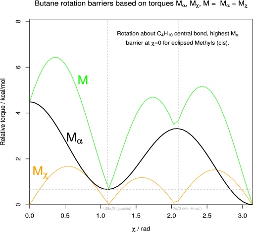
Figure 3: Butane torque barrier to rotation. Black curve with label M_α is the bond bending torque used for numerical examples in this work. Orange curve with label M_χ is torsional torque and green with label M is the sum M_α+M_χ. Vertical dashed lines mark reference angle values $(1.05*\pi/3,2\pi/3)$. The zero point (radians) corresponds to cis, $\chi=1.05*\pi/3$ to a staggered conformation producing a local minimum and $\chi=2\pi/3$ to an eclipsed conformation with a local peak. The horizontal dashed gray line corresponds to an experimental measurement of the gache₊ minimum at $1.05*\pi/3$, see text for reference. The angle value $\chi=\pi$ (anti or trans) has the lowest torque, which was defined as zero level. See Figure 2 for a definition of the torque components.

3.1.2 Related barriers to rotation

The set of parameters given in Table 3.1.4 were used to produce also other than the butane rotational barrier, to show that these tentative point charge parameters can be used more widely and get coherent results. In Figure 4, we show a comparison of the butane curve to two methyl-substituted butanes (2-methylbutane and 2,3-dimethylbutane). The gray dashed lines are the same as in Figure 3 and the curves approximately coinside at gauche₊, but 2-methylbutane gets a lower value at gauche_- ($\chi\approx-\pi/3$). In the torque model, this follows structurally from that 2-methylbutane has two staggered conformations without two instances of three consecutive Methyls or Hydrogens (as seen in a Newman projection), whereas butane and 2,3-methylbutane have only one such conformation (methyls or hydrogens in trans-conformation, respectively).

Barriers in light of rules from organic chemistry

The form of the torque barriers can be verified against textbook organic chemistry, e.g., the rules for estimating strain given in ref [28, p. 161]. Using those - 11 kJ/mol for eclipsed and 3.8 kJ/mol for gauche methyls (Me), 4 kJ/mol for H$\leftrightarrow$H and 6 kJ/mol for H$\leftrightarrow$Me eclipsed - produces the same functional forms for 2-methylbutane and 2,3-dimethylbutane as given in Figure 4 here.

In case of 2-methylbutane, the peak heights are quite close to those estimated with the mentioned directional rules (our 4.3 vs. 4.1 kcal/mol and our 3.0 vs. 3.4 kcal/mol). For 2,3-methylbutane the same are 5.3 vs. 4.4 kcal/mol and 4.1 vs. 3.7 kcal/mol, somewhat more different values. The joined gauche minimum torque for all three in Figure 4 is also produced by the strain rules [28, p. 161], but with a higher value of 0.9 kcal/mol as compared with the experimental value 0.67 kcal/mol form ref [27]. As mentioned, we used the latter as the most reliable fixed point for fitting the butane barrier to rotation.

3.1.3 Four ethane-type rotational curves

In Figure 5 is plotted ethane rotational curve with four other having the same general form, but different heights. In each of the four reference molecules, there is a methyl group at the other end of the rotatable bond studied, which produces the ethane-like torque profile. The strength is varied by groups bonded to the other end of the rotatable bond, and is highest for neopentane with three methyls bonded there. It is noted that the torque model, at least in the present form, handles a methyl as a carbon, which means specifying the covalent bond length and positions of parameter charges differently than, e.g., for a hydrogen at the other end of the rotating bond (see Table 3.1.4).

The lowest barriers are for methylamine, for which an adjustment to the parameters were made due to the amino groups, nitrogen having different electronegativity than carbon and (here) two hydrogens instead of the three in a methyl group. The adjustment was targeted to produce the barrier height that is about 2/3 of the ethane barrier calculated with the parameters in Table 3.1.4, 2.55 kcal/mol, to demonstrate applying the model.

3.1.4 Comparison with a quantum chemical two-diheral map

The third test for this set of parameters, in Table 3.1.4, is that they were used to produce the map for two consecutive straight chain alkane angles of rotation, representing the dihedrals $\chi_{3}$ and $\chi_{4}$ in lysine side chain.The result in Figure 6 was (visually) compared with a quantum chemically calculated map for two central diherals of n-pentane in ref [9]. Our torque map is both qualitatively and quantitatively a good match to the quantum chemically calculated torsion surface in figure 1 of article [9]. The only feature not observed in Figure 6 here, is the so called pentane interference, which is an interaction between parts of the alkane more distant than three bonds apart. In our framework, such interactions belong to external contacts (torque being defined as the internal or local).

Torque parameters used for calculating internal rotation preferences with respect to dihedrals $\chi_{2}$ - $\chi_{4}$ in lysine side chain. b / Å $\beta$ / degs. c / Å $\alpha$ / degs. qprod / e² $\chi_{0}$/degs. 0.7650 70.5 0.7650 70.5 3.31 -180 1.5300 70.5 1.5300 70.5 0.37 -180 0.7650 70.5 1.5300 70.5 -1.11 -180 1.5300 70.5 0.7650 70.5 -1.11 -180 0.7650 70.5 0.6867 70.5 3.31 -180 1.5300 70.5 1.0900 70.5 0.34 -180 0.7650 70.5 1.0900 70.5 -1.00 -180 1.5300 70.5 0.6867 70.5 -1.11 -180 0.7650 70.5 0.6867 70.5 3.31 -180 1.5300 70.5 1.0900 70.5 0.34 -180 0.7650 70.5 1.0900 70.5 -1.00 -180 1.5300 70.5 0.6867 70.5 -1.11 -180 0.6867 70.5 0.7650 70.5 3.31 -60 1.0900 70.5 1.5300 70.5 0.34 -60 0.6867 70.5 1.5300 70.5 -1.11 -60 1.0900 70.5 0.7650 70.5 -1.00 -60 0.6867 70.5 0.6867 70.5 3.31 -60 1.0900 70.5 1.0900 70.5 0.30 -60 0.6867 70.5 1.0900 70.5 -1.00 -60 1.0900 70.5 0.6867 70.5 -1.00 -60 0.6867 70.5 0.6867 70.5 3.31 -60 1.0900 70.5 1.0900 70.5 0.30 -60 0.6867 70.5 1.0900 70.5 -1.00 -60 1.0900 70.5 0.6867 70.5 -1.00 -60 0.6867 70.5 0.7650 70.5 3.31 60 1.0900 70.5 1.5300 70.5 0.34 60 0.6867 70.5 1.5300 70.5 -1.11 60 1.0900 70.5 0.7650 70.5 -1.00 60 0.6867 70.5 0.6867 70.5 3.31 60 1.0900 70.5 1.0900 70.5 0.30 60 0.6867 70.5 1.0900 70.5 -1.00 60 1.0900 70.5 0.6867 70.5 -1.00 60 0.6867 70.5 0.6867 70.5 3.31 60 1.0900 70.5 1.0900 70.5 0.30 60 0.6867 70.5 1.0900 70.5 -1.00 60 1.0900 70.5 0.6867 70.5 -1.00 60 Rotation about C_α-C_β ($\chi_{1}$) had a somewhat modified set due to not being alkane bond like. Model structure for estimating these parameters was n-butane. The tabulated values are to be taken strictly as suitable parameters for the torque model, not as estimates of, for example, the mean bond angle values. See Figure 2 for parameter definitions and text for details of estimating the parameters.

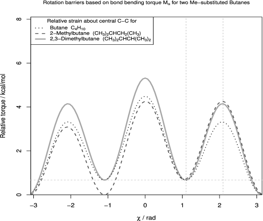
Figure 4: Calculated rotational barriers of methylated butanes, compared with that of n-butane. Structures were rotated internally about the central carbon-carbon bond and strain was calculated as bond bending torque (M_α). The strain at gauche₊ has the same value (0.67 kcal/mol) for all the three molecules. Torque at the other local minimum, gauche_- ($-2\pi/3$), is for 2-methylbutane the same as at trans-conformation, i.e., zero because the lowest torque is used as the base value. 2-Methylbutane has only one staggered conformation (gauche₊) with higher than minimum torque, due to asymmetry in groups over at the rotatable bond (two and one methyls bonded to the end atoms). Lowest strain for 2,3-methylbutane, i.e., trans-conformation or anti, is when the two hydrogens bonded to C₂ and C₃ are trans. The set of parameters given in text were used.

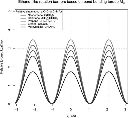
Figure 5: Bond bending torque rotational barrier for ethane and for internal rotations that have similar functional form of barrier in four other molecules. The molecules are rotated internally with respect to a methyl group in the structure. The figure shows how, in this model, a carbon-carbon (single) bond rotating at the other end of a rotatatable bond, experiences larger torque than a carbon-hydrogen bond. This then produces the result of higher barrier for eclipsed methyl group and hydrogen, than for eclipsed hydrogens. The set of parameters given in Table 3.1.4 were used, except an adjusted set for methylamine (lowest barrier) to obtain expected barrier height, which adjustment most likely produces a real difference due to the influence of the nitrogen (see text for details).

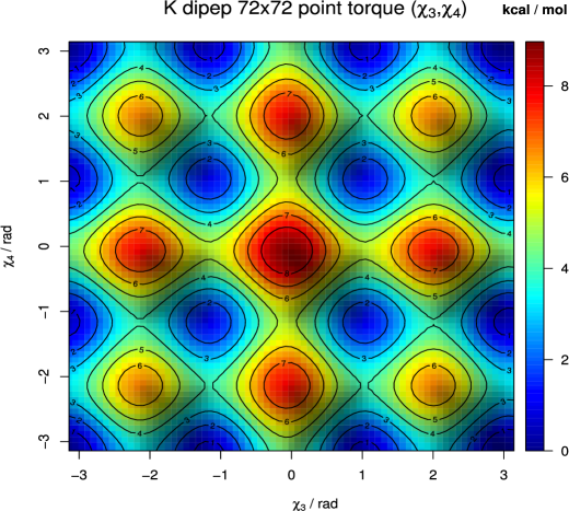
Figure 6: Torque map for angles ($\chi_{3}$,$\chi_{4}$) in lysine side chain, calculated as bond bending torque M_α. The corners correspond to trans-conformation for both dihedrals, about C_γ-C_δ and C_δ-C_ϵ.

3.1.5 Integration details

Target-atom distributions were in this work systematically generated through internal rotations about single bonds and modelled with a 3D kernel density estimate (see Equation 23). The bandwidth matrix $\mathbf{H}_{t}$ was evaluated for each thermal energy level (equals to torque cutoff) separately, using the default plug-in selector of the statistical modeling environment R package ’ks’ [25]. During the Riemann sum overlap calculations, the finite volume element $\Delta V=\frac{1}{3}(\rho_{i+1}^{3}-\rho_{i}^{3})(\cos(\theta_{j})-\cos(\theta_{j+1}))(\phi_{k+1}-\phi_{k})$ is kept constant by generating the variable values as the following sequences:

$$\rho_{i}=(i\,\frac{4}{3}\pi)^{\frac{1}{3}}\rho_{1},\>i=1,...,n_{\rho}$$

$$\theta_{j}=\arccos(1-j+j\cos(\theta_{1})),\>j=1,...,n_{\theta}$$ (25)

$$\phi_{k}=k\,\phi_{1},\>k=1,...,n_{\phi}$$

The values for parameters $\rho_{1},\theta_{1},\phi_{1}$ is a set of chosen starting values that determine the size of $\Delta V$.

3.2 Example: Conformational preferences in a lysine dipeptide

We have here as an exemplifying case a N-acetylated and N^’-methylamidated lysine dipeptide structure, shown in Figure 7 in two distinct side chain conformations. The dipeptide model structure was adapted from the work by Zhu et al. [29], where it was used as one of the targets for a quantum mechanical investigation of internal energy landscapes. Here, we use more degrees of freedom than in the original work and, in addition, study one internal noncovalent contact type in detail.

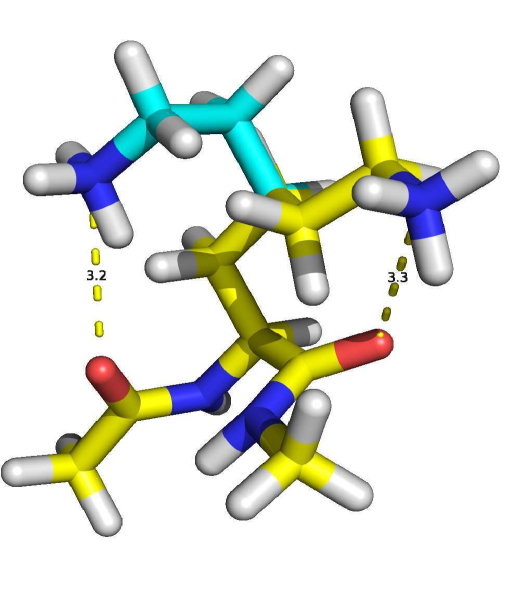
Figure 7: A lysine dipeptide model system. Main chain (mc) is for both contacts in a conformation corresponding to modest overlap. The angle values are ($\phi$,$\psi$)=(75,-30) degrees. This mc conformation is not necessarily internally favoured (see text for details), but is used to visualize the contact. Shown are also two side chain (sc) conformations that correspond to weak hydrogen bonds between sc amino nitrogen (NZ) and mc carbonyl oxygen. The side chain conformations experience internal torque that is less than 1.2 kcal/mol.

We will now focus on the lysine side chain NZ_i to main chain O_i-1,i contact. Subscript $i$ refers to the lysine residue in the dipeptide and O_i-1 is main chain carbonyl oxygen of the peptide bond. Common PDB atom names are used here as identifiers. The dipeptide structure is depicted in Figure 8 along with a modelled Target-atom (NZ_i) distribution and another cloud plot, for the contact preference density of the previous to lysine residue carbonyl. More precisely, the carbonyl group is part of the molecular fragment (O_i-1-C_i-1-N_i-1), with respect to which the reference frame of the contact preference density is determined.

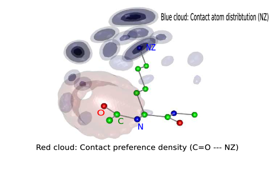
Figure 8: The model system with the 3D spatial probability densities that are factors in the overlap density. The contact preference of the fragment (O-C-N) is depicted as a red cloud, representing a cutoff of the density to show the approximate form. Target, or contact, atom (NZ) distribution modelled as a kernel density estimate, is shown as the blue patch-like clouds with darker areas corresponding to higher density values. Moving between patches is realized by the side chain conformation going thermally around maxima like the ones in Figure 6.

3.2.1 Internal scoring

Target atom distributions are based on internaltorque $M(\chi_{1},...,\chi_{n})=M(\chi_{1})+...+M(\chi_{n})$ and predefined thermal energy levels. Equation 5 determines a single term $M(\chi_{i})$, though only component $M_{\alpha}(\chi)$ used, as discussed. The thermal energy cutoffs for this study were chosen to be 1.0 and 1.2 kcal/mol, where the latter corresponds to an average kinetic energy of approximatelty 4(1/2)k_BT for the side chain (four bonds $\chi_{1},...,\chi_{4}$ are considered and T = 300 K). Conformations below these cutoffs might contain one or more less favoured rotational states about one of the four bonds, but the added bond-specific contributions produce the torque state, that is below the cutoff and the conformation is chosen for further use. In a more realistic case, these levels would be generated from a thermodynamic distribution, in which case the mean levels would be set according to temperature. Also, different degrees of freedom (rotatable bonds) can be given an individual response, in the form of a constraint restricting the freedom of motion, to the selected thermal energy. The response can for example be coupled to moment of inertia, as was done in ref [15] for an amino acid side chain. The average behaviour used in this work is considered to be precise enough for the purpose of presenting how the method is applied.

The dihedral pair ($\chi_{3}$,$\chi_{4}$)-dependent part of the side chain torque is exemplified in Figure 6. This torque map was calculated using M_α in Equation 5 and the tentative parameters given in Table 3.1.4. In the following examples, the term overlap is reserved for a purely attractive interaction, and contact preference is then obtained when the contact is evaluated with repulsion included.

3.2.2 Overlap for the terminal amino nitrogen

The generated distribution of lysine side chain nitrogen (NZ) positions was modeled with a 3D kernel density estimate, Equation 23. Values for the parameters used in the (main chain carbonyl oxygen) contact preference probability density, Equation 21, were estimated in our previous study [16]. The overlap integral was defined according to Equation 9 as an integral over the square root of the product of a kernel estimate and the contact preference density. Overlap values were obtained numerically as Riemann sums. The determined overlap profiles over a full rotation of both main chain rotatable angles $\psi$ and $\phi$ are shown in Figure 9.

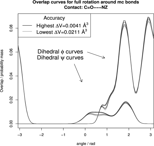
Figure 9: Five calculated overlap curves over trans$\rightarrow$trans rotation for both main chain dihedrals of the lysine, $\phi$ and $\psi$. Standard errors along mean curves (not shown) were SE$<$0.0019 for $\phi$ and SE$<$0.0014 for $\psi$. The inclusion of probabilistic repulsion to these curves produces what is here called contact preference. When defining calculation precision (pr) as the volume element size $\Delta V$, then 0.004$<$pr$<$0.021 $\AA^{3}$ for these curves.

Overlap profiles

The numerical overlaps over a full rotation, as shown in Figure 9, suggest that when the main chain dihedral angle $\psi$ (C-terminus side) has a value in the interval [0,2.2] rad or about [0,126] degrees, the lysine side chain nitrogen NZ forms the strongest contact to the main chain carbonyl oxygen (O_i). The $\psi$ values around 105^o or 1.83 rad (maximum overlap) turn the carbonyl group of the lysine residue to the same side with the side chain, which is a plausible conformation in order for a contact to form.

In the case of $\phi$ (N-terminus side), there are two almost equally high peaks, one at the same angle value as $\psi_{max}$ (1.83 rad) and the other, slightly higher peak, at 2.9 rad or 165 degrees. The steep gradient on both sides of both the $\phi$ angle maxima, follow from directional preferences in the side chain to main chain contact (NZ–O) and emphasize not to rely on only a single main chain conformation in computer models.

3.2.3 Side chain NZ preference for main chain C=O over full rotations

Repulsion was defined as negative probability in the section Interaction model. It should be mentioned, that extreme repulsion is not possible in our model, at least not without a unrealistically overcrowded spatial area, since the negative probability densities that we use do not tend towards infinity even when two atom centers coincide. This singularity is here prevented by simultaneously considering the effect of the whole space occupied by the entire conformer ensemble resulting from thermal motion, while still assigning relatively large repulsion for close contacts.

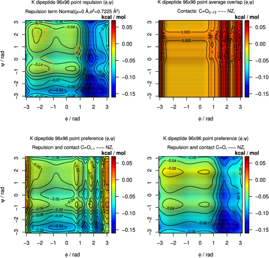
Figure 10: Factors of lysine dipeptide conformational preferences. Higher value on a surface means a more preferred point in dihedral ($\phi$,$\psi$) space. The surfaces are repulsion map (upper left), average overlap (upper right), preference with contact to previous residue carbonyl (lower left) and preference with contact to carbonyl of the same residue (lower right). Preference is calculated by adding the positive overlap probability mass to the negative probability surface of repulsion. Typical core areas of secondary structures ($\beta$,$\alpha_{R}$,$\alpha_{L}$) are marked with labeled ellipses. On the lower row, the effect of overlap mass is exaggerated due to not using a contact specific weight, for simplicity, but the form applies.

Figure 10 has four subfigures, and left on the upper row we show the normally distributed repulsion based ($\phi$,$\psi$)-map for our model system, lysine dipeptide. This map is a form of steric interaction based Ramachandran plot for lysine, though it should be remembered that the probabilistic repulsion model is a first approximation - an averaged distance dependent contact of main chain atoms with all generated side chain conformations simultaneously. Namely, ($\phi$,$\psi$)-torque, directional preferences and atom type specific features are to be included, but already this approximation gives reasonably the basic features like typical beta-conformations (marked with an ellipse) in the allowed, least repulsion area, and high repulsion on the $\phi>$60 degrees area. The latter follows from side chain to main chain interactions (not observed for glycine).

Average overlap probability masses (0.5*OL_ϕ+0.5*OL_ψ), produced by the side chain to main chain contacts (NZ_i to main chain O_i-1,i) are also plotted on the upper row in Figure 10. Starting from the repulsion surface on the left and the overlap probabilities, contact preferences (i.e., repulsion + overlap) relating to either of the calculated side chain to main chain interactions are shown on the lower row. Especially the contact that is dependent on the main chain dihedral $\phi$ (NZ_i to O_i-1, lower left), modifies strongly the repulsion based picture, which comes largely from that the sc to mc contacts are modelled separately as the only possible, giving them here the a priori weights of one. The weigth of the overlap for this contact was in our earlier work about 1/7.

Probability as a measure of preference

In general, like for total energy, the overall probability mass for an interaction complex comes from all plausible contacts, which are considered either simultaneous or alternative. The first of these is calculated by adding individual overlap masses, which quantifies how preferred the molecular environment, like a binding pocket is. In the second case, individual overlaps are compared to determine strengths of the contacts, and therefore the complex specific directional preferences. An example is the lysine side chain nitrogen being more preferred for the $\phi$-dependent carbonyl oxygen than for the $\psi$-dependent. Still added, that the highest Target-atom densities obtained for lysine NZ are when the side chain is pointing away from the main chain part, as depicted in Figure 8 by the blue clouds or patches. This means that contacts to the respective direction would get higher overlap probabilities, likely even when the contacts there would have lower weights C_i. As mentioned in the caption of Figure 10, the weights are not used in this work (see also Equation 10) for simplicity, because the spatial form of the overlap probability density is studied in this work and it is essential to all fragment classes.

The interaction complex specific directional aspect of the preferences is exemplified by that, when overlap masses to the previous residue carbonyl are added to the repulsion map (NZ_i to O_i-1, lower left in Figure 10), trans conformation is strongly preferred. This is isolated dipeptide specific and not seen in Ramachandran plots. The same features of the lower row surfaces would be there with an a priori weight, but less emphasized.

3.2.4 Referencing a quantum chemical result

A comparison of our overlap results with those of a quantum chemical calculation was done using the article [29], from which the model structure, or toy model, lysine dipeptide was picked. There the intrinsic energy of the dipeptide, mapped as 2D-function of first two side chain dihedrals ($\chi_{1}$,$\chi_{2}$) showed a deep well corresponding to $\beta$ and $\alpha_{L}$ main chain conformations. These deep wells were interpreted in ref [29] as due to a hydrogen bond between side chain and main chain, representing a way that mc conformation affects side chain internal preferences. Both, $\beta$ and $\alpha_{L}$, were in ref [29] represented by one mc dihedral angle point, and for $\beta$ had been chosen the angle values ($\phi$,$\psi$)=(-120,120) degs.
In our results, this mc conformation is in the band of highest $\psi$-dependent overlap probability mass, between 0.005-contours shown on the right on the upper row in Figure 10. The point is also in the most preferred area of least repulsion in ($\phi$,$\psi$)-space, when the contact from side chain to main chain of the same residue is added to repulsion (NZ_i — O_i, on the right on the lower row in Figure 10).

The other mc conformation, $\alpha_{L}$-helix, had in ref [29] been given the values ($\phi$,$\psi$)=(63.5,34.8) degs, which is a location (inside $\alpha_{L}$-ellipse in upper left map of Figure 10). In the lower left map, $\phi$-dependent contact NZ_i — O_i-1 overlap probability mass is added to negative probability mass of the upper left map and has compensated some of the repulsion in the $\alpha_{L}$ position, from -0.07 in upper left to -0.05 in lower left. This is in line with the lower intrinsic energy minimum for $\alpha_{L}$, given in ref [29] (supplementary), due to a side chain main H-bond.
The comparison is not straightforward, because in ref [29] had been varied two side chain dihedrals to produce the side chain conformations, whereas here we varied four. In addition, secondary structures were in ref [29] been represented by a single mc conformation and in this work full rotations were studied. Nevertheless, the quantum chemical work in ref [29] could be used as reference for our classical approach, which was one of the intended purposes of ref [29], as stated there.

The surfaces in Figure 10 would be altered by adding contacts to water molecules, or other small molecules or ions. Interactions involving these, like a water brigde, are in our approach modelled as mediated contacts, for an example, see [15].

3.2.5 About information content of overlap

As presented in this work, our conformational preference model gives the internal state of a molecular structure as torque. The thermal environment is in this treatment incorporated into the predictions by forcing a thermal energy level that gives the highest accessible torque value. To illustrate the effect that changing a level has, full $\phi$ and $\psi$ rotation overlap sets were calculated with a 1.0 kcal/mol cutoff, to be compared with the 1.2 kcal/mol used for the results otherwise in this work.

The results in Figure 11 (black and blue curves) match the presumption that the lower energy level produces a target distribution with lower overlap than the higher level. This follows from that the higher energy level cutoff allows the side chain to explore more conformations, which produces a larger overlap with the main chain fragment contact preference density for all $\phi$ and $\psi$ values. Only minor deviations are seen in the relative angle dependence between these curves based on two cutoffs, so mainly the magnitude of overlap varies in this case. Significant changes in the overlap shape are possible, and would depend on the internal torque of the structure, in which case those are part of the correct description of the system.

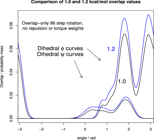
Figure 11: Compared overlap values for the lysine side chain nitrogen contact with main chain carbonyl oxygen. Contact over the $\phi$ and $\psi$ intervals corresponding to trans $\rightarrow$ trans rotation. Step size $\Delta\psi$ during rotation was $\pi$/48. Two thermal energy levels, 1.0 and 1.2 kcal/mol, used as cutoff for torque to vary accessible conformations in the target atom (NZ) distribution.

Space and time average

The rationale behind that an overlap integral incorporates the effect of structural flexibility, is that because conformations are generated based on internal preferences, no further than 1-4 interactions, the distribution contains all (classically) accessible structural conformations. Further, it is taken that when this distribution is modeled as a 3D probability density, the functional form describes both space and time average of conformational variation. The overlap integrand determines then how much of the conformational space, of the external contact free structure, is conserved in the contact. The roles of the interacting structures can be reversed and must produce the same results.

4 Discussion

We have previously constructed a probabilistic framework for modelling molecular interactions [16]. Relating to that, we introduce in the present work a torque-based model for scoring internal states or conformations, a negative probability density model for repulsive interactions, a new choice of densities to model Target-atom position distributions (in order to calculate overlap integrals that quantify the interactions) and an interpretation of the enthalpy–entropy compensation based on constant overlap probability mass.

We provide exemplifying calculations using butane, methylated butanes, alkanes like neopentane and a lysine dipeptide model system, in order to demonstrate the use of our method. The reasonableness of the numerical results obtained, using tentative parameters, was verified agains quantum chemical results from literature [9, 29] and well-known structural feature like allowed areas in a Ramachandran plot and approximate energy costs for eclipsed conformations in hydrocarbons.

Numerical integration of the overlap integrals at several different levels of precision produced values concentrated around a specific mean value, indicating that the results are robust in the tested numerical precision interval. The calculated overlap profiles change sharply, due to directional interaction preferences, in some of the studied angle intervals, indicating therefore that it is insufficient to present a peptide main chain secondary structure with only one ($\phi$,$\psi$)-conformation.

Further development of our method requires advances in the utilization of chemical information relevant for our model. A future challenge is a chemically precise molecular fragment classification. Such a classification may be based on quantum chemical or semi-empirical estimates for the local electronic structure. In the present model, contacts are classified as fragment–target interactions, however, a more elegant solution would be to formulate these directly as symmetric fragment–fragment interactions. Data collection for the improved interaction model update would then be based on the refined fragment classification, and the calculated electronic structure would be used to define new parameter charges for the torque model. In addition, combining different levels of internal motion in a macromolecule, in this framework, requires a separate scheme, e.g., due to different characteristic times of the respective conformation changes and interactions between more distant parts of the stucture.

In conclusion, our approach reduces the multidimensional problem of taking into account all plausible conformations in molecular interactions into three dimensions (at least locally) by formulating the interaction as an overlap integral of square roots of 3D probability densities. Therefore, this scoring function scheme provides an efficient way to incorporate thermal motion into a molecular model.

References

- [1] M. Gruebele and D. Thirumalai, J. Chem. Phys. 139, 121701 (2013).
- [2] C. Mura and C.E. McAnany, Mol. Simul. 40, 732 (2014).
- [3] J. Gao, D.G. Truhlar, Y. Wang, M.J.M. Mazack, P. Löffler, M.R. Provorse and P. Rehak, Acc. Chem. Res. 47, 2837−2845 (2014).
- [4] C. Forrey, J.F. Douglas and M.K. Gilson, Soft Matter 8, 6385 (2012).
- [5] G. Hernández, J.S. Anderson and D.M. LeMaster, Biophys. Chem. 163-164, 21 (2012).
- [6] T.W. Allen, O.S. Andersen and B. Roux, TThe Journal of General Physiology (JGP) 124 (6), 679 (2004).
- [7] H. Heinz, T.J. Lin, R.K. Mishra and F.S. Emami, Langmuir 29 (6), 1754 (2013).
- [8] S. Gasiorowicz, Quantum Physics (, , 1996).
- [9] J.M.L. Martin, J. Phys. Chem. A 117, 3118 (2013).
- [10] A.D. Mackerell, J. Comput. Chem. 25, 1584 (2004).
- [11] K. Lindorff-Larsen, S. Piana, K. Palmo, P. Maragakis, J.L. Klepeis, R.O. Dror and D.E. Shaw, Proteins 78 (8), 1950 (2010).
- [12] B.L. Eggimann, A.J. Sunnarborg, H.D. Stern, A.P. Bliss and J.I. Siepmann, Mol. Simul. 40, 101 (2014).
- [13] N. Andrusier, E. Mashiach, R. Nussinov and H.J. Wolfson, Proteins 73 (2), 271 (2008).
- [14] A.T. Tzanov, M.A. Cuendet and M.E. Tuckerman, J. Phys. Chem. B 118, 6539−6552 (2014).
- [15] R. Hakulinen, Ph.D. thesis, Åbo Akademi University, Åbo, Finland 2013.
- [16] R. Hakulinen, S. Puranen, J. Lehtonen, M. Johnson and J. Corander, PLoS ONE 7(11), e49216 (2012).
- [17] V.V. Rantanen, M. Gyllenberg, T. Koski and M.S. Johnson, J. Comput. Aided Mol. Des. 17 (7), 435 (2003).
- [18] J.R. Reitz, F.J. Milford and R.W. Christry, Foundations of Electromagnetic Theory (, , 1992).
- [19] T. Harder, W. Boomsma, M. Paluszewski, J. Frellsen, K.E. Johansson and T. Hamelryck, BMC Bioinformatics 11, 306 (2010).
- [20] G. Székely, Wilmott Magazine July, 66 (2005).
- [21] E. Wigner, Phys. Rev. 40, 749 (1932).
- [22] K. Sharp, Protein Sci. 10, 661 (2001).
- [23] J.D. Chodera and D.L. Mobley, Annu. Rev. Biophys. 42, 121 (2013).
- [24] A. Gelman, J.B. Carlin, H.S. Stern and D.B. Rubin, Bayesian Data Analysis (, , 2004).
- [25] T. Duong, ks: Kernel smoothing 2014, R package version 1.9.3.
- [26] Y. Mo, J. Org. Chem. 75, 2733 (2010).
- [27] W.A. Herrebout, B.J.v.d. Weken, A. Wang and J.R. Durig, J. Phys. Chem. 99, 578 (1995).
- [28] D. Klein, Organic Chemistry, 1st ed. (, , 2010).
- [29] X. Zhu, E.M. Lopes, J. Shim and A.D. MacKerell Jr., J. Chem. Inf. Model 52 (6), 1559 (2012).