A gamma approximation to the Bayesian posterior distribution of a discrete parameter of the Generalized Poisson model

Abstract

Let $X$ have a Generalized Poisson distribution with mean $kb$, where $b$ is a known constant in the unit interval and $k$ is a discrete, non-negative parameter. We show that if an uninformative uniform prior for $k$ is assumed, then the posterior distribution of $k$ can be approximated using the gamma distribution when $b$ is small.

1 Introduction

The family of Generalized Poisson distributions (GP) (Consul and Jain, 1973) has been used for more than 40 years to model count data that may be overdispersed or underdispersed. Some of its interesting theoretical properties include a Poisson mixture interpretation (Joe and Zhu, 2005), and a heavier tail compared to the negative binomial distribution (Joe and Zhu, 2005; Nikoloulopoulos and Karlis, 2008). Various chance mechanisms have been found to generate the GP distribution (Shoukri and Consul, 1987). Numerous applications are given in Consul (1989), and in recent years, it has gained increasing popularity in bioinformatics for modelling RNA-Seq count data (Srivastava and Chen, 2010; Li and Jiang, 2012; Zhang et al., 2015; Wang et al., 2015).

In this work, we study the posterior distribution of a discrete parameter of the GP model under a particular parametrization. Let $X$ be a random variable following $\mbox{GP}(\lambda_{1},\lambda_{2})$. Its probability mass function (pmf) is given by

$$P(X=x|\lambda_{1},\lambda_{2})=\frac{\lambda_{1}(\lambda_{1}+x\lambda_{2})^{x-1}e^{-(\lambda_{1}+x\lambda_{2})}}{x!}\ ,$$ (1)

where $x=0,1,2,\ldots$, $\lambda_{1}>0$ and $|\lambda_{2}|<1$. Negative values of $\lambda_{2}$ correspond to overdispersion, positive values to underdispersion, and $\lambda_{2}=0$ reduces eq.(1) to the Poisson distribution with mean $\lambda_{1}$. Consider the following parametrization: $\lambda_{2}=1-\sqrt{m}$, $\lambda_{1}=kb\sqrt{m}$, with $m=e^{ab+c}$. We assume that $a,c\in\mathbb{R}$ and $0<b<1$ are known constants, and focus our interest on the discrete non-negative parameter $k$. Under this parametrization, The mean and the variance of the GP model are given by

$$\mathbb{E}(X|k) = \lambda_{1}/(1-\lambda_{2})=kb\ ,$$

$$\mbox{Var}(X|k) = \mathbb{E}(X|k)/(1-\lambda_{2})^{2}=kb/m\ ,$$

We are concerned with the posterior probability of the $k$ parameter. In the absence of any prior information, a Bayesian formulation using an improper uniform prior $P(k)=1,k=0,1,2,\ldots$ on $k$ yields the posterior distribution of $k$ as

$$\begin{split}P(k|X=x)&=\frac{P(X=x|k)}{\sum_{j=x}^{\infty}P(X=x|j)}\\ &=\frac{k(bk\sqrt{m}+x(1-\sqrt{m}))^{x-1}e^{-bk\sqrt{m}}}{\sum_{j=x}^{\infty}j(bj\sqrt{m}+x(1-\sqrt{m}))^{x-1}e^{-bj\sqrt{m}}}\\ &=\frac{k(k+g(x))^{x-1}e^{-bk\sqrt{m}}}{\sum_{j=x}^{\infty}j(j+g(x))^{x-1}e^{-b\sqrt{m}j}},\\ \end{split}$$ (2)

for $k\geq x$, where $g(x)=\{(1-\sqrt{m})/(b\sqrt{m})\}x$. It is easy to check that $P(k|X=x)$ is proper even though an improper uniform prior distribution is used. The aim of this paper is to derive a continuous approximation to the posterior distribution eq.(LABEL:eq:posterior_gen), so that the posterior mean and variance can be determined directly from the theoretical properties of the approximating distribution.

2 Results

We show that under certain conditions, the gamma distribution approximates the posterior distribution of $k$.

Theorem 1.

If $P(k|X=x)$ is treated as a density function, then $P(k|X=x)$ is approximately equal to the probability density function of the gamma distribution with mean $(x+1)/(b\sqrt{m})$ and variance $(x+1)/(b^{2}m)$ for some $k\geq l$ where $l>x$.

Proof.

First, we note that the denominator in eq.(LABEL:eq:posterior_gen) can be written as

$$\sum_{j=x}^{\infty}(j+g(x))^{x}e^{-b\sqrt{m}j}-g(x)\sum_{j=x}^{\infty}(j+g(x))^{x-1}e^{-b\sqrt{m}j}.$$

The Lerch transcendent $\Phi(z,s,a)$ is given by

$$\Phi(z,s,a)=\sum_{k=0}^{\infty}\frac{z^{k}}{(a+k)^{s}},$$

where $|z|<1$, $a\neq 0,-1,-2,\ldots$, and $s\neq 1,2,\ldots$. Representing the denominator using the Lerch transcendent, we get

$$e^{-b\sqrt{m}x}\Phi(e^{-b\sqrt{m}},-x,wx)-(w-1)xe^{-b\sqrt{m}x}\Phi(e^{-b\sqrt{m}},-(x-1),wx),$$ (3)

where $w=1+(1-\sqrt{m})/(b\sqrt{m})$. The following identity (eq.1.11(11) in Erdélyi (1953)) relates the Lerch transcendent with negative argument for $s$ to the Bernoulli polynomials:

$$\Phi(z,-h,v)=\frac{h!}{z^{v}}\left(\log\frac{1}{z}\right)^{-(h+1)}-\frac{1}{z^{v}}\sum_{r=0}^{\infty}\frac{B_{h+r+1}(v)(\log z)^{r}}{r!(h+r+1)},$$ (4)

where $|\log z|<2\pi$, $v\neq 0,-1,-2,\ldots$, $h\neq-1,-2,\ldots$, and $B_{n}(x)$ is the $n$-th Bernoulli polynomial with argument $x$. The Bernoulli polynomial is defined as

$$B_{n}(x)=\sum_{j=0}^{n}{n\choose j}b_{n-j}x^{j},$$

where $b_{i}$ is the $i$th Bernoulli number. If we now substitute $z=e^{-b\sqrt{m}}$, $h=x$, $v=wx$ into the identity eq.(4), then we obtain

$$\Phi(e^{-b\sqrt{m}},-x,wx) = \frac{\Gamma(x+1)}{e^{-b\sqrt{m}(wx)}}(b\sqrt{m})^{-(x+1)}$$

$$-\frac{1}{e^{-b\sqrt{m}(wx)}}\sum_{r=0}^{\infty}\frac{B_{x+r+1}(wx)(-b\sqrt{m})^{r}}{r!(x+r+1)}$$

For small values of $b$ ($0<b<1$), we note that the sum of Bernoulli polynomials is dominated by the zero-th term. Hence, for the first term in eq.(3),

$$e^{-bw\sqrt{m}x}\Phi(e^{-b\sqrt{m}},-x,wx)=\frac{\Gamma(x+1)}{(b\sqrt{m})^{x+1}}-\frac{B_{x+1}(wx)}{x+1}+O(b\sqrt{m}),$$ (5)

as $b\rightarrow 0$. An identity involving the Bernoulli polynomials and the sum of $n$th powers (eq. 1.13(10) in Erdélyi (1953)) gives

$$\frac{B_{n+1}(x)-b_{n+1}}{n+1}=\sum_{r=0}^{x-1}r^{n}.$$

Since $B_{x+1}(x)$ dominates $b_{x+1}$, eq.(5) becomes

$$e^{-bw\sqrt{m}x}\Phi(e^{-b\sqrt{m}},-x,wx)\approx\frac{\Gamma(x+1)}{(b\sqrt{m})^{x+1}}-\sum_{r=0}^{[wx]-1}r^{x},$$

where $[wx]$ is the integer part of $wx$. Here,

$$e^{-bw\sqrt{m}x}\Phi(e^{-b\sqrt{m}},-x,wx)\approx\frac{\Gamma(x+1)}{(b\sqrt{m})^{x+1}},$$

provided that

$$\sum_{r=0}^{[wx]-1}r^{x}=o\left(\frac{\Gamma(x+1)}{(b\sqrt{m})^{x+1}}\right),$$

as $x\rightarrow\infty$. Now,

$$\frac{(b\sqrt{m})^{x+1}\sum_{r=0}^{[wx]-1}r^{x}}{\Gamma(x+1)} < \frac{b\sqrt{m}\{(bw\sqrt{m}x)^{x}+(bw\sqrt{m}x)^{x}+\cdots+(bw\sqrt{m}x)^{x}\}}{x!}$$

$$= \frac{(bw\sqrt{m}x)^{x+1}}{x!}$$

Let the upper bound on the right-hand-side be bounded by some constant $\epsilon>0$, which can be made arbitrarily close to 0. Thus, $(bw\sqrt{m}x)^{x+1}/x!<\epsilon$, and multiplying both sides by $x!$ and then taking logarithm, we get

$$[(1-\sqrt{m}+b\sqrt{m})x]<\exp\left\{\frac{1}{x+1}\left(\sum_{i=1}^{x}\log i+\log\epsilon\right)\right\}.$$ (6)

This implies that for some fixed $\epsilon$, the approximation should be reasonably good as long as $a,b,c$ and $x$ are such that the inequality (6) is satisfied.

For $a,b,c$ such that $\sqrt{m}\approx 1$, eq.(3) can be approximated as

$$\frac{\Gamma(x+1)}{(b\sqrt{m})^{x+1}}\left(1-(w-1)x\cdot\frac{b\sqrt{m}}{x}\right)\approx\frac{\Gamma(x+1)}{(b\sqrt{m})^{x+1}}.$$

It follows that the density function $P(k|X=x)$ (eq.(LABEL:eq:posterior_gen)) can be approximated using the probability density function of the gamma distribution with mean $(x+1)/(b\sqrt{m})$ and variance $(x+1)/(b^{2}m)$. Thus,

$$P(k|X=x) \approx \frac{(b\sqrt{m})^{x+1}k(k+g(x))^{x-1}e^{-b\sqrt{m}k}}{\Gamma(x+1)}$$

$$= \frac{k}{k+g(x)}\times\frac{(b\sqrt{m})^{x+1}(k+g(x))^{x+1-1}e^{-b\sqrt{m}k}}{\Gamma(x+1)}$$

$$\approx \frac{(b\sqrt{m})^{x+1}k^{x+1-1}e^{-b\sqrt{m}k}}{\Gamma(x+1)},$$

for $k\geq l$, since $g(x)=\{(1-\sqrt{m})/(b\sqrt{m})\}x$ and there exists some $l>x$, such that $k+g(x)=k+o(k)$ when $k\geq l$.

∎

Corollary 1.

For $k\geq l$, where $l>x$, the probability mass function $P(k|X=x)$ can be approximated as

$$P(k|X=x) \approx \int_{k-0.5}^{k+0.5}\frac{(b\sqrt{m})^{x+1}t^{x+1-1}e^{-b\sqrt{m}t}}{\Gamma(x+1)}dt$$

$$= \frac{1}{\Gamma(x+1)}\{\gamma(x+1,b\sqrt{m}(k+1/2))-\gamma(x+1,b\sqrt{m}(k-1/2))\},$$

where $\gamma(u,v)$ is the lower incomplete gamma function:

$$\gamma(u,v)=\int_{0}^{v}t^{u-1}e^{-t}dt.$$

2.1 Computational validation

The preceding results establish that the gamma family of distribution is a valid approximation to eq.(LABEL:eq:posterior_gen). Computational validation result suggests that an improvement to the fit can be obtained by replacing the shape and scale parameters of the gamma distribution in Theorem 1 as follows. Let $\mu_{post}$ and $\sigma^{2}_{post}$ be the posterior mean and the posterior variance, respectively. For a gamma distribution with shape parameter $\alpha$ and scale parameter $\beta$, its mean and variance are given by $\alpha\beta$ and $\alpha\beta^{2}$, respectively. Given $a,b,c$ and $x$, we can compute the exact mean and variance of the posterior distribution of $k$:

$$\mu_{post} = \sum_{k=x}^{\infty}kP(k|X=x),$$

$$\sigma^{2}_{post} = \sum_{k=x}^{\infty}k^{2}P(k|X=x)-\mu^{2}_{post}.$$

Simple algebra then yields $\alpha=\mu^{2}_{post}/\sigma^{2}_{post}$ and $\beta=\sigma^{2}_{post}/\mu_{post}$. The gamma approximation with $\alpha$ and $\beta$ thus computed fits eq.(LABEL:eq:posterior_gen) better than $\alpha=x+1$, $\beta=1/(b\sqrt{m})$ given in Theorem 1. Figure 1 shows the how well the gamma approximation fits the posterior distribution of $k$ with and without adjustment to $\alpha$ and $\beta$ parameters. In both cases the quality of the gamma approximation deteriorates when $x$ becomes relatively large if the $\alpha$ and $\beta$ parameters are not adjusted.

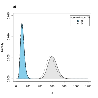
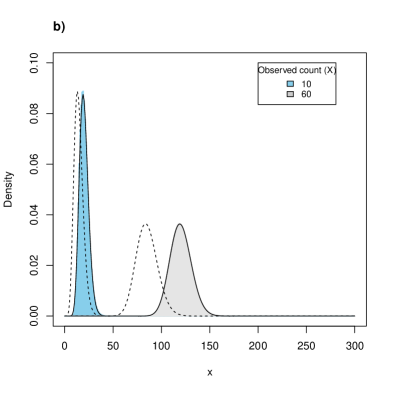
Figure 1: Examples of fitting the gamma distribution to the posterior distribution of $k$ for two cases: a) relatively small $b$ parameter: $a=1.5,b=0.1,c=-0.05$ ($m=1.1$); b) relatively large $b$ parameters: $a=1.5,b=0.5,c=-0.05$ ($m=2.0$). Solid lines indicate gamma approximation with shape and scale parameters determined by matching moments of the posterior distribution of $k$ and the gamma distribution. Broken lines indicate gamma approximation with shape and scale parameters given in Theorem 1.

3 Acknowledgment

I thank Martti Tammi and Joel Zi-Bin Low for stimulating the current work by discussing an applied problem in RNA-Seq count data analysis with me. Vanamamalai Seshadri read and provided feedback on the initial draft.

References

- Consul and Jain (1973) P. C. Consul, G. C. Jain, A generalization of the Poisson distribution., Technometrics 15 (1973) 791–799.
- Joe and Zhu (2005) H. Joe, R. Zhu, Generalized Poisson distribution: the property of mixture of Poisson and comparison with negative binomial distribution, Biometrical Journal 47 (2005) 219–229.
- Nikoloulopoulos and Karlis (2008) A. K. Nikoloulopoulos, D. Karlis, On modelling count data: a comparison of some well-known discrete distributions, Journal of Statistical Computation and Simulation 78 (2008) 437–467.
- Shoukri and Consul (1987) M. M. Shoukri, P. C. Consul, Some chance mechanisms generating the Generalized Poisson probability models, McGraw-Hill, New York, 1987.
- Consul (1989) P. C. Consul, Generalized Poisson Distribution: Properties and Applications, Marcel Dekker, New York, 1989.
- Srivastava and Chen (2010) S. Srivastava, L. Chen, A two-parameter generalized Poisson model to improve the analysis of RNA-Seq data, Nucleic Acids Research 47 (2010) 219–229.
- Li and Jiang (2012) W. Li, T. Jiang, Transcriptome assembly and isoform expression level estimation from biased RNA-Seq reads, Bioinformatics 28 (2012) 2914–2921.
- Zhang et al. (2015) J. Zhang, C. C. J. Kuo, L. Chen, WemIQ: an accurate and robust isoform quantification method for RNA-seq data, Bioinformatics 31 (2015) 878–885.
- Wang et al. (2015) Z. Wang, J. Wang, C. Wu, M. Deng, Estimation of isoform expression in RNA-seq data using a hierarchical Bayesian model, Journal of Bioinformatics and Computational Biology 13 (2015) 1542002.
- Erdélyi (1953) A. Erdélyi, Higher Transcendental Function Vol. I, McGraw-Hill, New York, 1953.