Quantum state-independent contextuality requires 13 rays

Abstract

We show that, regardless of the dimension of the Hilbert space, there exists no set of rays revealing state-independent contextuality with less than 13 rays. This implies that the set proposed by Yu and Oh in dimension three [Phys. Rev. Lett. 108, 030402 (2012)] is actually the minimal set in quantum theory. This contrasts with the case of Kochen–Specker sets, where the smallest set occurs in dimension four.

I Introduction

Fifty years ago, Kochen and Specker KS67 answered the following question: Is it possible that, independently of which is the quantum state, the quantum observables each possess a definite single value, regardless of whether they are measured or not? The Kochen–Specker (KS) theorem states that this is impossible if the dimension of the underlying Hilbert space is larger than two. One consequence of this theorem is the impossibility of reproducing quantum theory in terms of noncontextual hidden variable theories, defined as those in which the outcomes are independent of the context. A context is a set of mutually compatible quantum observables. In this sense, quantum theory is said to exhibit contextuality.

The original proof of the KS theorem had two other distinctive traits: (i) It only used a finite set of observables with two outcomes, where one outcome is represented by a rank-one projection onto a ray of the Hilbert space. Hereafter, as it is common in the literature, we will use ray as synonym of self-adjoint rank-one projection. (ii) The set is KS-uncolorable, i.e., it is impossible to assign values 1 or 0 to each ray while respecting that two orthogonal rays cannot both have assigned 1, and 1 must be assigned to exactly one of $d$ mutually orthogonal rays. These restrictions are motivated by the observation that orthogonal rays correspond to mutually exclusive outcomes of a sharp observable and $d$ mutually orthogonal rays correspond to an exhaustive set of mutually exclusive outcomes for a Hilbert space of dimension $d$. KS-uncolorable sets of rays are called KS sets PMMM05 .

The original KS set had 117 rays in $d=3$, which can be grouped in 132 contexts. There have been many efforts for finding simpler sets exhibiting state-independent contextuality (SIC). For instance, Peres and Mermin realized that, by considering observables not represented by rank-one projections and replacing KS uncolorability by a similar condition, one can find very compact sets of observables in $d=4$ and $d=8$ Peres90 ; Mermin90 . Still, these sets can be rewritten in terms of KS sets Peres91 ; KP95 . So far, it has been shown PMMM05 that the KS set of minimum cardinality occurs in $d=4$ and has 18 rays CEG96 . It also has been proved PMMM05 that, in $d=3$, the KS set with minimum cardinality has more than 22 and less than 32 rays CK95 . On the other hand, the KS set with minimum number of contexts known occurs in $d=6$ and has seven contexts (and 21 rays) LBPC14 .

A big step was the observation that SIC based on rays does not need to rely on KS-uncolorable sets. It is enough that they lead to a state-independent violation of a noncontextuality inequality. This substantially simplifies the methods for revealing SIC in $d=3$. Specifically, Yu and Oh singled out one set with 13 rays in $d=3$ YO12 . The optimal state-independent noncontextuality inequalities for this set were identified in Ref. KBLGC12, . Sets of rays having a state-independent violation of a non-contextuality inequality are called SIC sets.

Recent experiments testing SIC KZGKGCBR09 ; ARBC09 ; MRCL10 ; ZWDCLHYD12 ; ZUZ13 ; DHANBSC13 ; CEGSXLC14 ; CAEGCXL14 ; JRO16 and an increasing number of applications, such as device-independent secure communication HHHHPB10 , local contextuality Cabello10 ; LHC16 , Bell inequalities revealing full nonlocality AGACVMC12 , state-independent quantum dimension witnessing GBCKL14 , and state-independent hardware certification CAEGCXL14 , have stimulated the interest in the following question: Which is the minimal set of rays needed for SIC? It is known that, for $d=3$, the answer is 13 CKB15 , but it would be well possible that the minimal set occurs in some higher dimension, as it happens for KS sets. Here we prove that this is not the case.

II Main result

The basis of our proof is a condition identified by Ramanathan and Horodecki RH14 ; CKB15 to be necessary for any SIC set in dimension $d$, namely that the orthogonality graph $G$ of the set of rays has fractional chromatic number $\chi_{f}(G)>d$. The orthogonality graph of a SIC set is the graph in which orthogonal rays are represented by adjacent vertices. A coloring of $G$ is an assignment of colors to the vertices such that adjacent vertices are associated with different colors. $\chi_{f}(G)$ is the infimum of $\frac{a}{b}$ such that vertices have a set of $b$ associated colors, out of $a$ colors, where adjacent vertices have associated disjoint sets of colors.

Instead of considering all possible SIC sets of size $n$, we rather investigate all graphs with $n$ vertices. Then, we consider the nondegenerate orthogonal representations (ORs) of any graph $G$. An OR is an injection $\phi$, mapping the vertices of $G$ to rays, such that adjacent vertices in $G$ are mapped to orthogonal rays. The OR is faithful (FOR) if, conversely, any two orthogonal rays correspond to an edge of $G$. We denote by ${\Xi}(G)$ the smallest dimension of the Hilbert space which still admits a FORs of $G$. It then follows from the Ramanathan–Horodecki condition that $G$ is the orthogonality graph of a SIC set only if $\chi_{f}(G)>{\Xi}(G)$. Our main results is then as follows.

Theorem 1.

Any graph $G$ with 12 or less vertices has $\chi_{f}(G)\leq{\Xi}(G)$.

Hence, according to quantum theory, no SIC set with less than 13 rays exists.

III Proof of Theorem 1

We proceed by an exhaustive search for a counterexample, examining all $166\,122\,463\,890$ nonisomorphic graphs with up to 12 vertices. Applying a cascade of filters we eventually discard all graphs and prove this way Theorem 1. We start by introducing the criteria for defining these filters and then explain our procedure providing intermediate results for each of the filters.

We denote by $V(G)$ and $E(G)$ the sets of vertices and edges of $G$, respectively. The complement $\overline{G}$ of $G$ is a graph that has the same vertices while the edges are the complemented set, i.e., $e\in E(\overline{G})$ if and only if $e\notin E(G)$. A subgraph $S$ of $G$ is any graph with $V(S)\subset V(G)$ and $E(S)\subset E(G)$. A subgraph is induced if $\overline{S}$ is also a subgraph of $\overline{G}$. It is a simple observation that any (F)OR is also a (F)OR of any (induced) subgraph. Defining ${\xi}$ analogously to ${\Xi}$, but for ORs, this proves the following.

Lemma 2.

By definition, ${\xi}(G)\leq{\Xi}(G)$. If $S$ is a subgraph of $G$, then ${\xi}(S)\leq{\xi}(G)$. Similarly, if $S$ is an induced subgraph of $G$, then ${\Xi}(S)\leq{\Xi}(G)$.

The union of two graphs $G_{1}\cup G_{2}$ consists of the disjoint union of the respective vertex sets and edge sets. The join $G_{1}+G_{2}$ of two graphs is the union of both graphs adding one edge between any pair $(v_{1},v_{2})\in V(G_{1})\times V(G_{2})$. The graph $K_{1}$ with one vertex and no edge takes a special role in the following simple relations.

Lemma 3.

For two graphs $G_{1}$ and $G_{2}$ and $f\in\set{\chi_{f},{\Xi},{\xi}}$, we have $f(G_{1}\cup G_{2})=\max[f(G_{1}),f(G_{2})]$ and $f(G_{1}+G_{2})=f(G_{1})+f(G_{2})$, with the exceptions ${\Xi}(K_{1}\cup K_{1})=2$ and ${\xi}(K_{1}\cup K_{1})=2$.

Proof.

For $\chi_{f}$ the relations are well-known, cf., e.g., Ref. Scheinerman:1997, , Sec. 3.10. For ${\Xi}$ and ${\xi}$ and the first relation, the maximum is at least a lower bound, since any (F)OR of $G_{1}\cup G_{2}$ must also be a (F)OR of $G_{1}$ and of $G_{2}$. Conversely, if at least one of the graphs has more than one vertex then also its (F)OR has at least dimension two. This (F)OR can then be transformed by a unitary rotation, such that the image of the (F)ORs of $G_{1}$ and $G_{2}$ are disjoint and also no rays are orthogonal. Hence one can combine any two (F)ORs of $G_{1}$ and $G_{2}$ to a (F)OR in the larger of the dimensions of both (F)ORs. The second relation follows at once, noting that $\set{v_{1},v_{2}}\in E(G_{1}+G_{2})$ if and only if either $v_{1}\in V(G_{1})$ and $v_{2}\in V(G_{2})$, or vice versa, or $\set{v_{1},v_{2}}\in E(G_{1})$, or $\set{v_{1},v_{2}}\in E(G_{2})$. Hence $\phi$ is a (F)OR for $G_{1}+G_{2}$ if and only if it is a (F)OR for $G_{1}$ and $G_{2}$, and the spans of $\phi[V(G_{1})]$ and $\phi[V(G_{2})]$ are mutually orthogonal. ∎

These relations are useful for our purposes since they imply that, if a graph or its complement is not connected and $\chi_{f}(G)>{\Xi}(G)$, then this must already be true for a subgraph of $G$. Hence in our search we only need to consider connected graphs the complement of whose are also connected. Another important consequence of Lemma 3 is that ${\xi}(n\overline{K_{2}}+mK_{1})=2n+m$, where $K_{\ell}$ is the completely connected graph with $\ell$ vertices Solis:2012 ; Solis:2015XXX . This implies ${\Xi}(G)\geq 2n+m$ as soon as $n\overline{K_{2}}+mK_{1}$ is a subgraph of $G$. A weaker form of this condition is that if $K_{\ell}$ is a subgraph of $G$, then ${\Xi}(G)\geq\ell$.

Graph name	In Fig. 1	graph6	${\Xi}$	Filter	Remaining
$\overline{H}$	(a)	Ebtw	5	(3.1)	$124\,220$
$\operatorname{Ci}_{8}(1,2)$	(b)	Gbijmo	5	(3.2)	$124\,216$
$\overline{H}+K_{1}$	—	Fbvzw	6	(3.3)	$4\,722$
$\overline{\operatorname{Caterpillar}_{2}^{3,2}}$	(c)	Fbtzw	6	(3.4)	569
$\overline{\operatorname{Caterpillar}_{3}^{2,1,1}}$	(d)	Fbuzw	6	(3.5)	400
$\operatorname{Ci}_{11}(1,2,3)\setminus\set{v}$	(e)	Ibgzmngjg	6	(3.6)	366
$\overline{H}+K_{2}$	—	Gzznnk	7	(3.7)	0

Table 1: List of graphs used for filtering via Lemma 2. The graphs $\operatorname{Caterpillar}_{k}^{n_{1},\dotsc,n_{k}}$ are linear graphs of length $k$, where $n_{v}$ leafs are added to vertex $v$. $H=\operatorname{Caterpillar}_{2}^{2,2}$, $\operatorname{Ci}_{n}(e_{1},\dotsc,e_{m})$ is the circulant graph, where each vertex is connected to its $e_{1}$th-, …, $e_{m}$th-next neighbor. $G\setminus\set{v}$ is the graph $G$ with one vertex removed. Selected graphs are displayed in Fig. 1. graph6 is a standard graph data format widely used in computer software graph6 . The number ${\Xi}$ is the smallest dimension of any faithful nondegenerate orthogonal representation. The last column shows the number of graphs remaining after filtering for the induced subgraph, cf. main text.

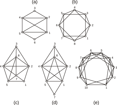
Figure 1: Graphs from Table 1. Graphs (a) and (b) have ${\Xi}=5$ and graphs (c)–(e) have ${\Xi}=6$. The other two graphs from Table 1 are obtained by adding one or two vertices to graph (a) each being connected to all other vertices.

As a final ingredient to our proof, we use the seven graphs listed in Table 1. If any of those graphs is an induced subgraph $S$ of $G$, then ${\Xi}(G)\geq{\Xi}(S)$ applies. The values of ${\Xi}(S)$ are obtained by construction, and due to Lemma 3 it is sufficient to study the five graphs in Fig. 1. The construction is similar for all five graphs and we demonstrate the method only for the most complicated case $\operatorname{Ci}_{11}(1,2,3)\setminus\set{v}$, cf. Fig. 1 (e). The vertices $\set{4,5,6,7}$ form the induced subgraph $K_{4}$ and, without loss of generality, we can choose $\phi(4)=(1,0,0,0,0)$, $\phi(5)=(0,1,0,0,0)$, $\phi(6)=(0,0,1,0,0)$, and $\phi(7)=(0,0,0,1,0)$. Since vertex 3 is adjacent to the vertices $\set{4,5,6}$ and not adjacent to vertex 7 or 8, and vertex 7 is adjacent to 8, we have $\phi(3)=(0,0,0,a,1)$ with some $a\neq 0$. By similar arguments, $\phi(2)=(0,0,b,-1/a^{*},1)$ with $b\neq 0$, and, by symmetry, $\phi(8)=(c,0,0,0,1)$ and $\phi(9)=(-1/c^{*},d,0,0,1)$, with $c,d\neq 0$. Using, that vertex 1 is adjacent to the vertices $\set{4,9,3,2}$, we have $\phi(1)=(0,-1/d^{*},-x/b^{*},-1/a^{*},1)$ with $x=1+1/{\lvert{a}\rvert}^{2}$, and, by symmetry, $\phi(10)=(-1/c^{*},-y/d^{*},-1/b^{*},0,1)$ with $y=1+1/{\lvert{c}\rvert}^{2}$. Eventually, vertex 1 and 10 are adjacent, implying $y/{\lvert{d}\rvert}^{2}+x/{\lvert{b}\rvert}^{2}+1=0$, which is a contradiction. However, it is straightforward to find a FOR in dimension 6, proving ${\Xi}[\operatorname{Ci}_{11}(1,2,3)\setminus\set{v}]=6$.

For all graphs with less than 13 vertices, we discard those graphs which satisfy at least one of the following filter criteria:

(1)	$G$ or $\overline{G}$ is not connected.
(2.1)	$G$ has subgraph $K_{\ell}$, where $\chi_{f}(G)\leq\ell$.
(2.2)	$G$ has subgraph $n\overline{K_{2}}+mK_{1}$, where $\chi_{f}(G)\leq 2n+m<\chi_{f}(G)+1$ and $m\in\set{0,1}$.
(3.1)–(3.7)	$G$ has an induced subgraph $S$ from Table 1 with $\chi_{f}(G)\leq{\Xi}(S)$.

For obvious reasons, we fall back to a computer-based proof. We use geng from the software package nauty nauty14 ; nauty to generate all nonisomorphic graphs. The fractional chromatic number can be obtained by solving the linear program Scheinerman:1997 ; SDT0 ,

$$\begin{split}\text{maximize:}&\sum_{v\in V(G)}x_{v}\\ \text{subject to:}&\sum_{v\in\mathcal{I}}x_{v}\leq 1,\text{ for all $\mathcal{I}$ of $G$}\\ &x_{v}\geq 0\text{ for all $v\in V(G)$},\end{split}$$ (1)

where $\mathcal{I}$ are independent sets of $G$, i.e., sets of vertices where all vertices are mutually nonadjacent. We find optimal solutions to this program using the software package GLPK GLPK and verify the correctness of the solution by applying the strong duality of linear programs, using an accuracy threshold of $\epsilon=10^{-12}$. We approximate the floating-point value obtained for $\chi_{f}$ by a rational number with less than $\epsilon$ deviation, while constraining the denominator to be not larger than $nm$, where $n$ is the number vertices of $G$ and $m$ is the number of maximal independent sets. This procedure always succeeds and ensures that the calculation of $\chi_{f}$ is exact, despite floating-point arithmetic being used in intermediate steps.

order	graphs	(1)	(2.1)	(2.2)
1	1	1	0	0
2	2	0	0	0
3	4	0	0	0
4	11	1	0	0
5	34	8	1	0
6	156	68	2	0
7	$1\,044$	662	28	0
8	$12\,346$	$9\,888$	456	0
9	$274\,668$	$247\,492$	$15\,954$	3
10	$12\,005\,168$	$11\,427\,974$	$957\,882$	98
11	$1\,018\,997\,864$	$994\,403\,266$	$99\,869\,691$	$5\,765$
12	$165\,091\,172\,592$	$163\,028\,488\,360$	$19\,715\,979\,447$	$560\,500$

Table 2: Number of nonisomorphic graphs with 1–12 vertices. (1)–(2.2) after filtering, cf. main text.

We apply all filters (1)–(3.7) consecutively so that each filter reduces the number of candidate graphs. The numbers of graphs remaining after each step are shown in Table 2, for filters (1), (2.1), and (2.2), and as a function of the number of vertices of the graph. The list of $566\,366$ graphs remaining after filter (2.2) is available in graph6-format data . For the filters (3.1)–(3.7), we show in Table 1 the total number of remaining graphs after each filter. No graph remains after applying all filters, which proves Theorem 1.

IV Conclusions

Contextuality is a fundamental feature of quantum observables and can be completely detached from any features of the quantum state of the system. This state-independent contextuality already occurs for the most elementary case of observables being sharp and having only two outcomes, one of which is nondegenerate; such observables can be represented by rays in a Hilbert space. Here we have shown that state-independent contextuality with elementary observables requires at least 13 different observables by performing an exhaustive search over all cases with less observables. The Yu–Oh set is an example of such 13 observables and is already realizable on a three-level quantum system, which is the smallest quantum system allowing for contextuality. This is in contrast to the first instances of state-independent contextuality, the Kochen–Specker sets, where the smallest set cannot be realized on a three-level system. Therefore, fifty years after the discovery of state-independent contextuality in quantum theory, we finally have the answer to the question of which is the simplest way to reveal it, i.e., which is the smallest set of elementary observables exhibiting state-independent contextuality.

- (1) S. Kochen and E. P. Specker, The problem of hidden variables in quantum mechanics, J. Math. Mech. 17, 59 (1967).
- (2) M. Pavičić, J.-P. Merlet, B. D. McKay, and N. D. Megill, Kochen–Specker vectors, J. Phys. A: Math. Gen. 38, 1577 (2005).
- (3) A. Peres, Incompatible results of quantum measurements, Phys. Lett. A 151, 107 (1990).
- (4) N. D. Mermin, Simple unified form for the major no-hidden-variables theorems, Phys. Rev. Lett. 65, 3373 (1990).
- (5) A. Peres, Two simple proofs of the Kochen–Specker theorem, J. Phys. A: Math. Gen. 24, L175 (1991).
- (6) M. Kernaghan and A. Peres, Kochen–Specker theorem for eight-dimensional space. Phys. Lett. A 198, 1 (1995).
- (7) A. Cabello, J. M. Estebaranz, and G. García-Alcaine, Bell–Kochen–Specker theorem: A proof with 18 vectors, Phys. Lett. A 212, 183 (1996).
- (8) J. H. Conway and S. Kochen, reported in A. Peres, Quantum Theory: Concepts and Methods (Kluwer, Dordrecht, 1995), p. 114.
- (9) P. Lisoněk, P. Badziąg, J. R. Portillo, and A. Cabello, Kochen–Specker set with seven contexts, Phys. Rev. A 89, 042101 (2014).
- (10) S. Yu and C. H. Oh, State-independent proof of Kochen–Specker theorem with 13 rays, Phys. Rev. Lett. 108, 030402 (2012).
- (11) M. Kleinmann, C. Budroni, J.-Å. Larsson, O. Gühne, and A. Cabello, Optimal inequalities for state-independent contextuality, Phys. Rev. Lett. 109, 250402 (2012).
- (12) G. Kirchmair, F. Zähringer, R. Gerritsma, M. Kleinmann, O. Gühne, A. Cabello, R. Blatt, and C. F. Roos, State-independent experimental test of quantum contextuality, Nature (London) 460, 494 (2009).
- (13) E. Amselem, M. Rådmark, M. Bourennane, and A. Cabello, State-independent quantum contextuality with single photons, Phys. Rev. Lett. 103, 160405 (2009).
- (14) O. Moussa, C. A. Ryan, D. G. Cory, and R. Laflamme, Testing contextuality on quantum ensembles with one clean qubit, Phys. Rev. Lett. 104, 160501 (2010).
- (15) C. Zu, Y.-X. Wang, D.-L. Deng, X.-Y. Chang, K. Liu, P.-Y. Hou, H.-X. Yang, and L.-M. Duan, State-independent experimental test of quantum contextuality in an indivisible system, Phys. Rev. Lett. 109, 150401 (2012).
- (16) X. Zhang, M. Um, J. Zhang, S. An, Y. Wang, D.-L. Deng, C. Shen, L.-M. Duan, and K. Kim, State-independent experimental test of quantum contextuality with a single trapped ion, Phys. Rev. Lett. 110, 070401 (2013).
- (17) V. D’Ambrosio, I. Herbauts, E. Amselem, E. Nagali, M. Bourennane, F. Sciarrino, and A. Cabello, Experimental implementation of a Kochen–Specker set of quantum tests, Phys. Rev. X 3, 011012 (2013).
- (18) G. Cañas, S. Etcheverry, E. S. Gómez, C. Saavedra, G. B. Xavier, G. Lima, and A. Cabello, Experimental implementation of an eight-dimensional Kochen–Specker set and observation of its connection with the Greenberger–Horne–Zeilinger theorem, Phys. Rev. A 90, 012119 (2014).
- (19) G. Cañas, M. Arias, S. Etcheverry, E. S. Gómez, A. Cabello, G. B. Xavier, and G. Lima, Applying the simplest Kochen–Specker set for quantum information processing, Phys. Rev. Lett. 113, 090404 (2014).
- (20) M. Jerger, Y. Reshitnyk, M. Oppliger, A. Potočnik, M. Mondal, A. Wallraff, K. Goodenough, S. Wehner, K. Juliusson, N. K. Langford, and A. Fedorov, Contextuality without nonlocality in a superconducting quantum system, eprint arXiv:1602.00440.
- (21) K. Horodecki, M. Horodecki, P. Horodecki, R. Horodecki, M. Pawłowski, and M. Bourennane, Contextuality offers device-independent security, eprint arXiv:1006.0468.
- (22) A. Cabello, Proposal for revealing quantum nonlocality via local contextuality, Phys. Rev. Lett. 104, 220401 (2010).
- (23) B.-H. Liu, X.-M. Hu, J.-S. Chen, Y.-F. Huang, Y.-J. Han, C.-F. Li, G.-C. Guo, and A. Cabello, Experimental test of the free will theorem, eprint arXiv:1603.08254.
- (24) L. Aolita, R. Gallego, A. Acín, A. Chiuri, G. Vallone, P. Mataloni, and A. Cabello, Fully nonlocal quantum correlations, Phys. Rev. A 85, 032107 (2012).
- (25) O. Gühne, C. Budroni, A. Cabello, M. Kleinmann, and J.-Å. Larsson, Bounding the quantum dimension with contextuality, Phys. Rev. A 89, 062107 (2014).
- (26) A. Cabello, M. Kleinmann, and C. Budroni, Necessary and sufficient condition for quantum state-independent contextuality, Phys. Rev. Lett. 114, 250402 (2015).
- (27) R. Ramanathan and P. Horodecki, Necessary and sufficient condition for state-independent contextual measurement scenarios, Phys. Rev. Lett. 112, 040404 (2014).
- (28) P. J. Cameron, A. Montanaro, M. W. Newman, S. Severini, and A. Winter, On the quantum chromatic number of a graph, Electr. J. Comb. 14, #R81 (2007).
- (29) E. R. Scheinerman and D. H. Ullman, Fractional Graph Theory. A Rational Approach to the Theory of Graphs (John Wiley & Sons, New York, 1997).
- (30) A. Solís, Algoritmos para la Resolución del Problema de Representación Ortogonal (Master Thesis, Universidad de Sevilla, 2012)
- (31) A. Solís and J. R. Portillo, Orthogonal representation of graphs, eprint arXiv:1504.03662.
- (32) B. D. McKay and A. Piperno, Practical graph isomorphism, II, J. Symb. Comput. 60, 94 (2014).
- (33) nauty and Traces, http://pallini.di.uniroma1.it/.
- (34) D. Bertsimas and J. N. Tsitsiklis, Introduction to Linear Optimization (Athena Scientific, Belmont, Massachusetts, 1997).
- (35) GNU Linear Programming Kit, http://www.gnu.org/software/glpk/.
- (36) http://personal.us.es/josera/minSIC/, sha256-digest a23b d030 d126 a3e5 44c0 f820 afcf aa9a ac31 a991 4ae1 416a 6a1a 682f 9bbe 2535.
- (37) B. D. McKay, Description of graph6 and sparse6 encodings, http://cs.anu.edu.au/~bdm/data/formats.txt.