A multistate dynamic site occupancy model for
spatially aggregated sessile communities

Abstract

Inferring transition probabilities among ecological states is fundamental to community ecology because, based on Markovian dynamics models, these probabilities provide quantitative predictions about community composition and estimates of various properties that characterize community dynamics. Markov community models have been applied to sessile organisms because such models facilitate estimation of transition probabilities by tracking species occupancy at many fixed observation points over multiple periods of time. Estimation of transition probabilities of sessile communities seems easy in principle but may still be difficult in practice because resampling error (i.e., a failure to resample exactly the same location at fixed points) may cause significant estimation bias. Previous studies have developed novel analytical methods to correct for this estimation bias. However, they did not consider the local structure of community composition induced by the aggregated distribution of organisms that is typically observed in sessile assemblages and is very likely to affect observations. In this study, we developed a multistate dynamic site occupancy model to estimate transition probabilities that accounts for resampling errors associated with local community structure. The model applies a nonparametric multivariate kernel smoothing methodology to the latent occupancy component to estimate the local state composition near each observation point, which is assumed to determine the probability distribution of data conditional on the occurrence of resampling error. By using computer simulations, we confirmed that an observation process that depends on local community structure may bias inferences about transition probabilities. By applying the proposed model to a real dataset of intertidal sessile communities, we also showed that estimates of transition probabilities and of the properties of community dynamics may differ considerably when spatial dependence is taken into account. Our approach can even accommodate an anisotropic spatial correlation of species composition, and may serve as a basis for inferring complex nonlinear ecological dynamics.

Key words: Classification error; Community dynamics; Hierarchical models; Intertidal; Kernel smoothing; Site occupancy models; Spatial correlation; Transition probability

INTRODUCTION

Markov models are a general class of mathematical models that are widely used to describe dynamics of ecological systems. In the context of community ecology, they offer a simple and useful representation of community dynamics. For example, a very basic Markov model summarizes the dynamics of a community (i.e., changes in community composition or site occupancy dynamics among ecological states) with a transition matrix, $\mathbf{P}$, which consists of the transition probability from state $k$ to $j$, $p_{jk}$, in the element in its $j$ th row and $k$ th column. Such linear Markov models may not provide a fully realistic description of community dynamics in nature, which may be inherently nonlinear (Spencer and Tanner 2008, Tanner et al. 2009). Nevertheless, they can still provide a good approximation of observed community dynamics and composition (Wootton 2001a, b, Hill et al. 2002). Linear Markov models also allow us to assess a wide range of properties of species-level dynamics (e.g., rate of colonization, disturbance, and replacement) as well as those of community-level dynamics (e.g., equilibrium community composition, as well as its sensitivities, mean turn over time, and damping ratio), which can be derived from the transition probability matrix (Hill et al. 2004).

Markov community models have been applied to communities of sessile organisms (e.g., terrestrial plants, corals and intertidal/subtidal communities) because in those systems transition probabilities can be estimated with field data by tracking species occupancy at many fixed observation points over multiple periods of time (e.g., Wootton 2001a, b, Hill et al. 2002, 2004, Tanner et al. 2009). However, estimation of transition probabilities may be biased when there are resampling errors, that is, failures to resample exactly the same fixed-point locations. When such a resampling error occurs, researchers observe a point that is different from, but probably close to, the correct location of the fixed point; the result may be a “misclassification” of the occupancy state. Such an error may sometimes be inevitable in field sampling, where somewhat crude tools are necessarily used and/or organisms are small (Conway-Cranos and Doak 2011). New analytical methods have been proposed to correct this estimation bias which assume that the probability distribution of data, conditional on the occurrence of resampling error, is related to the relative state frequency of ecological states (Conway-Cranos and Doak 2011, Fukaya and Royle 2013). On the one hand, Conway-Cranos and Doak (2011) proposed a maximum likelihood approach, in which transition probabilities and resampling error rates are estimated based on multinomial likelihoods. On the other hand, Fukaya and Royle (2013) proposed to use the dynamic site occupancy modeling framework to account for resampling error in the estimation of transition probabilities.

In both of these studies, spatial aspects of community structure were not considered explicitly. It is very likely, however, that the local structure of community composition affects the observation process described above, because sessile organisms typically represent locally aggregated spatial distributions. Therefore, accounting for such spatial dependence will be necessary to make more reliable inferences about underlying community dynamics. In this study, we developed an extension of the multistate dynamic site occupancy model proposed by Fukaya and Royle (2013) to account for spatial dependence in the estimation of transition probabilities. We used additional information about the spatial coordinate of each observation point to estimate the state composition near each point. Estimation of this local community structure was possible by applying the nonparametric multivariate kernel smoothing methodology (Diggle et al. 2005) to the latent occupancy component. Our approach can even account for an anisotropic spatial correlation of species composition and may also lead to some potential extensions of the model, which we describe in the Discussion. By using computer simulations, we confirmed that an observation process that depends on local community structure may cause some bias in the inference of transition probabilities. By applying the proposed model to a real dataset of intertidal sessile communities, we also showed that estimates of transition probabilities and of community dynamics may be considerably different when spatial dependence is accounted for.

THE MODEL

Model description

We assumed that there were, in total, $I$ fixed observation points within a permanent quadrat that could be occupied by one of the possible $S$ ecological states (species or groups of species, which may include “free space”). Hence, observation points and the quadrat corresponded to “sites” (local populations) and the “meta-population”, respectively, in the meta-population design concept for the site occupancy modeling framework (Kéry and Schaub 2012, Kéry and Royle 2016). The ecological state was assessed for each site over $T$ periods of time. We define $z_{it}$ and $y_{itn}$ ($z_{it},y_{itn}\in 1,\dots,S$) as the occupancy state at site $i$ ($i=1,\dots,I$) at time $t$ ($t=1,\dots,T$), and the state observed by a researcher (i.e., data recorded) at the $n$th measurement ($n=1,\dots,N(i,t)$) at site $i$ at time $t$, respectively. The $N(i,t)$ observations consisted of replicated samples at site $i$ and time $t$; these samples may have been collected by repeated surveys conducted within a sufficiently short period or by independent observers. This sampling scheme formally resembles Pollock’s robust design, which is classically considered in capture-recapture studies (Pollock 1982) in which secondary resampling is performed within a single primary sampling period ($t$). We note that the dynamic site occupancy modeling framework described below also permits missing data.

Changes in site occupancy states ($z_{it}$) across primary sampling periods are described with a transition probability matrix $\mathbf{P}$. The element in the $j$ th row and $k$ th column $p_{jk}(1\leq j,k\leq S)$ represents the transition probability from state $k$ to $j$. Resampling error probability $e$ is also considered to account for a certain type of observation error that arises when there is failure to resample the exact location of the fixed observation site (Conway-Cranos and Doak 2011). It is thus assumed that when resampling error does not occur at a sampling occasion for site $i$ at time $t$ (occurring with a probability $1-e$), the occupancy state $z_{it}$ is recorded with probability 1, whereas when resampling error occurs, the “occupancy state” observed is a random variable that follows a certain probably distribution (Fukaya and Royle 2013). Fukaya and Royle (2013) assumed that when a resampling error occurs, the probability of state $s$ being observed is equal to the relative dominance of that state within the quadrat, $f_{ts}=\sum_{i}\bm{1}(z_{it}=s)$, where $\bm{1}(x)$ is an indicator function. Conceptually, this assumption implicitly requires that organisms are homogenously distributed within the quadrat so that the state composition is identical over all sites. The same assumption was made by Conway-Cranos and Doak (2011) to account for a similar type of resampling error in longitudinal observations of sessile communities. To account for the spatial dependence of community structure, we here consider the relative dominance of the state near each site, $g_{its}$, and relate it, instead of $f_{ts}$, to the data distribution conditional on the occurrence of the resampling error.

Although the model framework could accommodate more ecological realities, we here restricted our model by using the simplest elements possible for notational simplicity and clarity. We believe this approach will facilitate understanding the basic model structure. Possible extensions of the model are described in the Discussion. Formally, the model we propose is as follows.

Observation model — We assume that on each sampling occasion, with probability $(1-e)$, observers assess the exact location of site $i$ and find the true occupancy state $z_{it}$. But otherwise (i.e., with probability $e$), they fail to observe the exact location of that site. In the latter case, we assume that they record state $s$ with a probability that equals the local dominance of that state, $g_{its}$. This observation distribution, conditional on the occurrence of the resampling error, represents a categorical distribution with a probability vector $(g_{it1},\dots,g_{itS})$. With a latent indicator variable $m_{itn}$ representing the occurrence of resampling error for the $n$th measurement at site $i$ at time $t$, the model for this observation process is expressed as:

$$y_{itn} =z_{it} m_{itn}=0$$ when (1)

$$y_{itn} \sim\textrm{Categorical}(g_{it1},\dots,g_{itS}) \text{when $m_{itn}=1$}.$$

We assume that resampling errors occur independently, and thus that $m_{itn}$ simply follows a Bernoulli distribution:

$$m_{itn}\sim\textrm{Bernoulli}(e).$$ (2)

Process model — Assuming that the dynamics of the occupancy state is a Markov process, the conditional probability of latent state $z_{it}$ for $t=2,3,\dots,T$ can be expressed as follows:

$$z_{it}|(z_{i,t-1}=s)\sim\textrm{Categorical}(p_{1s},p_{2s},\dots,p_{Ss}),$$ (3)

where $p_{js}$ gives the transition probability from state $s$ to $j$. The transition probability matrix $\mathbf{P}$ is expressed as follows:

$$\mathbf{P}=\begin{pmatrix}p_{11}&\dots&p_{1s}&\dots&p_{1S}\\ \vdots&\ddots&\vdots&&\vdots\\ p_{s1}&\dots&p_{ss}&\dots&p_{sS}\\ \vdots&&\vdots&\ddots&\vdots\\ p_{S1}&\dots&p_{Ss}&\dots&p_{SS}\end{pmatrix}$$ (4)

where column $s$ gives the vector of transition probabilities for $z_{it}|(z_{i,t-1}=s$). Note that this transition probability matrix is column-stochastic (i.e., each column sums to 1).

For $t=1$, the initial occupancy probability of each site is defined by a probability vector $\bm{\phi}=(\phi_{1},\dots,\phi_{S})$. The model for initial occupancy states is thus expressed as:

$$z_{i1}\sim\textrm{Categorical}(\phi_{1},\dots,\phi_{S}).$$ (5)

A kernel estimator for the local state composition — The local state dominance $g_{its}$ is unobserved, and we now describe a model for $g_{its}$. We estimate $g_{its}$ nonparametrically by using a multivariate kernel smoothing methodology to estimate the spatial structure of multinomial probabilities (Diggle et al. 2005).

We let $\mathbf{x}_{i}$ be a two-dimensional coordinate vector for site $i$. For each $i$, $t$, and $s$, the kernel regression estimator for the local state composition is expressed as follows:

$$g_{its}=\frac{\sum_{j=1}^{I}K_{\bm{\Sigma}}(\mathbf{x}_{i},\mathbf{x}_{j})\bm{1}(z_{jt}=s)}{\sum_{r=1}^{S}\sum_{j=1}^{I}K_{\bm{\Sigma}}(\mathbf{x}_{i},\mathbf{x}_{j})\bm{1}(z_{jt}=r)},$$ (6)

where $z_{jt}$ is the latent occupancy state at site $j$ at time $t$, and $K_{\bm{\Sigma}}(\mathbf{x}_{i},\mathbf{x}_{j})$ is a two-dimensional Gaussian kernel function with a bandwidth matrix $\mathbf{\Sigma}$:

$$K_{\bm{\Sigma}}(\mathbf{x}_{i},\mathbf{x}_{j})=\exp\left\{-\frac{1}{2}(\mathbf{x}_{i}-\mathbf{x}_{j})^{\prime}\mathbf{\Sigma}^{-1}(\mathbf{x}_{i}-\mathbf{x}_{j})\right\}.$$ (7)

The bandwidth matrix $\mathbf{\Sigma}$ is a $2\times 2$ positive definite covariance matrix:

$$\mathbf{\Sigma}=\begin{pmatrix}\sigma_{1}^{2}&\rho\sigma_{1}\sigma_{2}\\ \rho\sigma_{1}\sigma_{2}&\sigma_{2}^{2}\end{pmatrix},$$ (8)

where $\sigma_{1},\sigma_{2}>0$ is the scale parameter for each dimension and $-1<\rho<1$ is the correlation parameter. Note that the assumption of a common kernel function across ecological states simplifies the estimator (Eq. 6) as follows:

$$g_{its}=\frac{\sum_{j=1}^{I}K_{\bm{\Sigma}}(\mathbf{x}_{i},\mathbf{x}_{j})\bm{1}(z_{jt}=s)}{\sum_{j=1}^{I}K_{\bm{\Sigma}}(\mathbf{x}_{i},\mathbf{x}_{j})}.$$ (9)

With the kernel estimator of this form, $g_{its}$ becomes higher at site $i$ as the number of sites that are occupied by state $s$ at time $t$ increases. Although all the sites occupied by $s$ at time $t$ contributes to $g_{its}$, the weight decreases as a function of the distance from site $i$: the scale of this distance dependence is controlled by the bandwidth matrix $\mathbf{\Sigma}$. We note that $\mathbf{\Sigma}$ accounts for an anisotropic spatial dependence (i.e., direction dependence) of the local community structure: the spatial dependence is isotropic only when $\sigma_{1}=\sigma_{2}$ and $\rho=0$.

As long as there is no significant sources of observation error other than the resampling error we considered above, the estimated vector $(g_{it1},\dots,g_{itS})$ is interpreted naturally as a representation of the composition of ecological states surrounding site $i$ at time $t$. As in Fukaya and Royle (2013), $g_{its}$ is a derived parameter obtained as a function of latent occupancy state {$z_{it}$}, whereas the function defining $g_{its}$ now depends on an unknown bandwidth matrix with parameters to be estimated. We also note that when the bandwidth of the kernel is sufficiently large, $g_{its}$ will no longer vary over sites within the quadrat. The result is a spatially homogeneous situation that is equivalent to the model considered by Fukaya and Royle (2013).

Estimation of states and parameters

In this model, elements of the transition probability matrix $\mathbf{P}$, the resampling error rate $e$, the initial occupancy probability vector $\bm{\phi}$, and the elements of the bandwidth matrix $\bm{\Sigma}$ are parameters to be estimated. The model also involves occupancy state $z_{it}$, error occurrence indicator $m_{itj}$, and the local state composition $g_{its}$ (a derived quantity) as latent state variables. The model assumes that observation at a particular time point depend on all the state variables at that time. Such a class of dynamic models is called a factorial hidden Markov model in the machine learning community, and for such a model it is known that an exact likelihood inference is computationally intractable (Ghahramani and Jordan 1997). We thus adopt here a Bayesian approach for parameter inference, in which the joint posterior distribution of parameters and latent state variables is obtained by using Markov chain Monte Carlo (MCMC) methods. We specify vague priors for parameters for the observation and process models:

$$e\sim\textrm{Beta}(1,1),$$ (10)

$$(p_{1s},\dots,p_{Ss})\sim\textrm{Dirichlet}(1,\dots,1),$$ (11)

$$(\phi_{1},\dots,\phi_{S})\sim\textrm{Dirichlet}(1,\dots,1),$$ (12)

where the diffuse Dirichlet prior (Eq. 11) is specified for each of column $s$ of the transition probability matrix. Vague priors would also be specified for elements of the bandwidth matrix, $\bm{\Sigma}$, as follows:

$$\sigma_{1} \sim\textrm{Uniform}(0,U)$$ (13)

$$\sigma_{2} \sim\textrm{Uniform}(0,U)$$ (14)

$$\rho\sim\textrm{Uniform}(-1,1)$$ (15)

where $U$ is a sufficiently large positive constant defining the upper limit of the uniform prior.

The joint posterior distribution of these parameters and latent variables ({$z_{it}$}, {$m_{itn}$}, {$g_{its}$}) can be obtained by using the MCMC methods. The model can be implemented using the BUGS software. We have provided a model script in the Appendix that can be used to fit the model using JAGS software (Plummer 2003).

SIMULATION STUDY

Materials and methods

To examine the effect of an observation process that is relevant to the local community structure on the inference of community dynamics, we conducted a simulation study. Using the system and observation models described above, with fixed model parameters that were to be estimated, we simulated a number of replicate datasets that were obtained from the hierarchical data-generating process described in the previous section. Simulations and analyses described in what follows were conducted using R (versions 3.1.0 to 3.2.5).

Three models were fitted to these simulated data sets. The first was a classical, naive estimator for transition probabilities, defined as $\hat{p}_{jk}=n_{jk}/\sum_{l}n_{lk}$, where $n_{jk}$ is the number of sites that were in state $k$ at a certain point in time and in state $j$ at the following time (Spencer and Susko 2005). This model does not account for any type of observation error. The second was a “non-spatial” multistate dynamic site occupancy model proposed by Fukaya and Royle (2013), which does account for resampling errors. The model assumes that the distribution of the observed state, conditional on the occurrence of the resampling error, is proportional to the relative dominance of each state in the quadrat that is homogeneous in space. Finally, the “spatial” multistate dynamic site occupancy model described in the previous section was also fitted to simulated datasets. Note that this model is equivalent to the data-generating model and was thus expected to perform the best among the three models.

To generate replicated datasets, we set the number of sites $I=225$, the length of time series $T=5$, and the number of ecological states $S=5$. The sites were assumed to be aligned on a $15\times 15$ grid, and their coordinates were represented as $\mathbf{x}_{1}=(1,1),\mathbf{x}_{2}=(2,1),\dots,\mathbf{x}_{225}=(15,15)$. We used a transition probability matrix that was randomly drawn from a diffuse Dirichlet distribution $(p_{1s},\dots,p_{Ss})\sim\textrm{Dirichlet}(1,\dots,1)$. For the observation process, we assumed an isotropic bandwidth kernel by setting $\sigma_{1}=\sigma_{2}=1$ and $\rho=0$. With these settings, we generated 96 replicate datasets for each of 6 levels of error rate ($e=0,0.15,0.3,0.45,0.6$, $0.75$).

We considered two scenarios for the manner of data collection. The first scenario considered a situation of limited information where no replicated observations were obtained; that is, we set $N(i,t)=1$ for all $i$ and $t$. The second scenario simulated a more ideal situation where three replicated observations were conducted for each survey; that is, we set $N(i,t)=3$ for all $i$ and $t$.

Among the three models and two sampling scenarios described above, the performances of the models were evaluated based on the mean square error (MSE), square of bias ($\textrm{Bias}^{2}$) and variance (Var) of the point estimate of each parameter. For transition probabilities, the above criteria were averaged over all elements in the probability matrix to evaluate the magnitude of the estimation errors in a sequence of transition probabilities. Because MSE measures the mean square difference of estimates from the true parameter value, it may serve as a comprehensive criterion for the quality of estimators. The MSE can be decomposed into bias and variance, as the three are linked by the relationship $\textrm{MSE}(\hat{\theta})=\textrm{Bias}^{2}(\hat{\theta})+\textrm{Var}(\hat{\theta})$. Thus, we favor a model with a lower MSE, and such a model may even be better if it provides less biased estimates.

For the naive model, data were simply aggregated to $n_{jk}$ to obtain estimates of transition probabilities. Because this model does not accommodate replicated sampling, it was not applied to data from the three-replicate scenario. For the non-spatial and spatial model, parameters were estimated using the Bayesian inference framework. For each analysis of replicated datasets, we specified a vague prior for each parameter (Eqs. 10–15) to sample from the posterior distribution using the JAGS software (versions 3.4.0 to 4.2.0; Plummer 2003), from three independent chains of 3000 iterations after a burn-in of 3000 iterations thinning at intervals of 3. The posterior mode was used for point estimates of univariate parameters ($e$ and $\sigma$), whereas the spatial median was used for transition probabilities to ensure that the sum of each column of the probability matrix was 1.

Convergence of the posterior was checked for each parameter with the Gelman-Rubin diagnostic $\hat{R}$. In the spatial model, about 0.03% of the estimates of $p_{jk}$, 9% of $e$ (most of which came from small $e$ situations, where estimation of $\sigma$ was difficult; see the next subsection), and 12% of $\sigma$ (same as $e$) had $\hat{R}>1.2$. In the non-spatial model, about 0.3% of $p_{jk}$ and 5% of $e$ had $\hat{R}>1.2$. Although these $\hat{R}$ values may not be appropriate in formal model inference (e.g., Gelman et al. 2014), we considered our results to be acceptable for examination of the average performance of the model using the simulated dataset. In practice, the $\hat{R}$ values could be improved by much longer MCMC runs, which can be very time-consuming in the context of simulation but would not be prohibitive for analysis of one or a small number of datasets.

Results

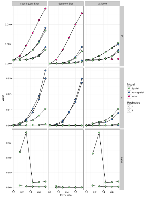
Figure 1: Results of simulation study. Mean square error (left column), square of bias (middle column), and variance (right column) of parameter estimates obtained from 96 replicated datasets using three different models (spatial model, non-spatial model, and naive estimator) are shown. Upper, middle, and lower panels indicate results for the transition probability matrix $\hat{\mathbf{P}}$, resampling error rate $\hat{e}$ and the bandwidth scale parameter $\hat{\sigma}$, respectively. Results of $\hat{\sigma}$ for $e=0$ in the spatial model are not shown because of a convergence issue (see text for details).

The results of the simulation study are summarized in Fig. 1. We first note that when the error rate is small, the posterior distribution for the bandwidth parameter $\sigma$ in the spatial model sometimes failed to converge. In such cases, the posterior distribution of $\sigma$ was typically distributed over a wide range, a reflection of the flat specified prior distribution, the result being spatially homogeneous estimates of the local state composition $g_{its}$. This result suggests an identification issue for $\sigma$ in these settings, an issue that appears to become worse when replicated samples are lacking (Fig. 1). In the spatial model, $\sigma$ determines the probability distribution of data conditional on the occurrence of resampling error. Hence, $\sigma$ is not satisfactorily determined by data when resampling errors occur infrequently. Even when the posterior sampling for $\sigma$ was unsuccessful, however, the convergence of other parameters in the spatial model ($\mathbf{P}$ and $e$) was typically achieved. In these cases, estimates of transition probabilities were often very similar in the spatial model and the non-spatial model. This similarity reflects the fact that the estimated local state composition $g_{its}$ was spatially homogeneous, the result being a spatial model that was virtually the same as the non-spatial model, in which a spatially homogeneous state composition was assumed implicitly.

For this reason, we excluded estimates from the calculation of MSE, bias, and variance of $\hat{\sigma}$, if the difference between the point estimate and the true value of $\sigma$ was more than 10 (Fig. 1, lower panels). We omitted the results of MSE, square bias, and the variance of $\hat{\sigma}$ for $e=0$ because this procedure excluded almost all estimates for $e=0$. We also note that in the spatial model with $e=0$ and three replicated observations, there was an estimate of $e$ that was exceptionally large. We also excluded that estimate from the calculation of MSE, bias, and variance of $\hat{e}$.

Not surprisingly, overall, the bias was the smallest in the spatial model compared to other models (Fig. 1). When comparisons were made among the results of the single-replicate case, estimates of transition probabilities from the naive estimator were the least variable (Fig. 1, upper panels). However, the estimator became profoundly biased as the error rate increased, the result being the worst MSE of the transition probabilities among the examined models. The bias and variance of the transition probability estimates in the non-spatial and spatial model increased with the error rate. The bias of the transition probabilities was considerably smaller in these models compared to the naive model, resulting in the better MSE as the error rate increased. Although the difference between the non-spatial and spatial models in the estimation of transition probabilities is not so large, the bias and MSE of the spatial model was smaller than that of the non-spatial model when the error rate was high (i.e., $e\geq 0.45$). Replicated observations improved the estimation of transition probabilities in the spatial and non-spatial model. Under these conditions, the performance of the non-spatial model was even better than that of the spatial model with a single replicate.

The MSE of $\hat{e}$ tended to be higher for the non-spatial model than for the spatial model (Fig. 1, middle panels) because the bias of the non-spatial model increased faster than that of the spatial model, although the variance of $\hat{e}$ was in general smaller in the non-spatial model than in the spatial model. In the non-spatial model, replicated observations did not mitigate the MSE and bias of $\hat{e}$. In the spatial model, the MSE and bias of $\hat{\sigma}$ tended to be higher when the error rate was low (Fig. 1, lower panels), where, as noted above, the estimation of $\sigma$ may be difficult.

In summary, these results suggest that, when the local community structure affects observations, both the naive estimator and the non-spatial multistate dynamic site occupancy model may provide worse estimates than the spatial model. When the error rate is low, the bandwidth parameter of the spatial model may not be satisfactorily determined by data, but the model may still perform as well as the non-spatial model by estimating the spatially homogeneous relative state composition. As the error rate increased, the spatial model on average outperformed the non-spatial model.

APPLICATION TO REAL DATA

Materials and methods

We applied the proposed spatial model, in addition to the non-spatial model (Fukaya and Royle 2013) and the naive estimator for transition probabilities (Spencer and Susko 2005), to an intertidal sessile community dataset collected at a total of 25 permanent quadrats within 5 shores — Mochirippu (MC), Mabiro (MB), Aikappu (AP), Monshizu (MZ) and Nikomanai (NN)— located on the Pacific coast of eastern Hokkaido, Japan (detailed descriptions of the study sites and biogeographic features of the area can be found in Okuda et al. 2004, Nakaoka et al. 2006 and Fukaya et al. 2014). Each quadrat was established on rock walls at semi-exposed locations and was 50 cm wide by 100 cm high. The vertical mid-point corresponded to the mean tidal level. In each quadrat, 200 fixed observation points (i.e., sites) were aligned on 20 horizontal rows by 10 vertical columns. The sites were located at intervals of 5 cm. Site occupancy dynamics of ecological states were assessed once per year from 2002 to 2011, during a spring low tide in the summer (from roughly July to August).

Table 1: Parameter estimates (transition probability matrix $\mathbf{P}$, resampling error probability $e$, and bandwidth matrix $\bm{\Sigma}$) obtained by fitting each of the three different models (naive estimator, non-spatial model, and spatial model) to the intertidal sessile community dataset of a particular quadrat (MC2). Posterior medians are reported for the spatial and non-spatial models, for which posterior sampling was conducted using MCMC. The rows and columns of the transition probability matrix correspond to: (1) free space, (2) the barnacle Chthamalus dalli, (3) the red alga Gloiopeltis furcata, (4) the articulated calcareous red alga Corallina pilulifera, and (5) other organisms.

	Model
Parameter	Naive	Non-spatial	Spatial
$\mathbf{P}$	$\begin{bmatrix}0.560&0.328&0.375&0.051&0.164\\ 0.085&0.267&0.100&0.020&0.082\\ 0.320&0.339&0.446&0.020&0.143\\ 0.006&0.013&0.003&0.471&0.156\\ 0.028&0.053&0.076&0.438&0.455\end{bmatrix}$	$\begin{bmatrix}0.670&0.221&0.307&0.013&0.028\\ 0.064&0.416&0.100&0.014&0.016\\ 0.258&0.328&0.585&0.011&0.020\\ 0.003&0.005&0.002&0.501&0.196\\ 0.005&0.029&0.006&0.461&0.740\end{bmatrix}$	$\begin{bmatrix}0.772&0.160&0.208&0.015&0.040\\ 0.053&0.574&0.060&0.016&0.029\\ 0.165&0.239&0.713&0.015&0.037\\ 0.003&0.008&0.002&0.684&0.098\\ 0.007&0.020&0.017&0.270&0.796\end{bmatrix}$
$e$		$0.239$	$0.715$
$\mathbf{\Sigma}$			$\mbox{diag}(0.644,1.278)$

Models were fitted to estimate transition probabilities for each quadrat. In the study sites, we recognized the following seven dominant ecological states: (1) free space, (2) the barnacle Chthamalus dalli, (3) the brown alga Analipus japonicus, (4) the red alga Gloiopeltis furcata, (5) the red alga Chondrus yendoi, (6) the articulated calcareous red alga Corallina pilulifera, and (7) other organisms. However, states 1–6 were not necessarily common in each quadrat. Thus, for each quadrat, we allocated some of these regionally dominant states to state 7 (other organisms) when they were relatively rare (when the total number of their occurrences during the 10 observation years was $<50$) in that quadrat. As a result, the number of states varied from 4 to 7 among quadrats.

For each quadrat, models were fitted to data in a fashion analogous to that used in the simulation study described in the previous section. To fit the spatial model, we restricted the bandwidth matrix to $\bm{\Sigma}=\textrm{diag}(\sigma_{1}^{2},\sigma_{2}^{2})$, where $\sigma_{1}$ and $\sigma_{2}$ were the scale parameters along the vertical and horizontal directions, respectively. For spatial and non-spatial models, we first conducted MCMC sampling for each plot with three independent chains of 3000 iterations after a burn-in of 3000 iterations, thinning at intervals of 3. For some plots, however, we needed to have longer iterations and more chains to obtain converged posterior samples. The convergence of parameters of interest was confirmed if the Gelman-Rubin diagnostic $\hat{R}$ was less than 1.1. We note, however, that for MB4, AP4 and AP5, we could not obtain converged posterior samples of $\sigma_{2}$, probably because the spatial dependency along the horizontal axis was lacking or because there were insufficient data to estimate it.

As derived parameters, we also obtained estimates of two quantities that inform some dynamical aspects of communities: the mean turnover time and the damping ratio (Hill et al. 2004). The former quantifies the average turnover time of a site randomly selected from the stationary community. It is calculated as $\sum_{s=1}^{S}w_{s}(1-p_{ss})^{-1}$ where $w_{s}$ is the equilibrium relative dominance of state $s$ obtained as the normalized dominant right eigenvector of the transition probability matrix $\mathbf{P}$. The latter quantifies the lower bound of the rate of convergence to equilibrium. It is equated to $1/|\lambda_{2}|$ where $\lambda_{2}$ is the second-largest eigenvalue of $\mathbf{P}$.

Results

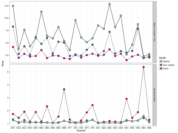
Figure 2: Mean turnover time (upper panel) and damping ratio (lower panel) estimated using three models (spatial model, non-spatial model, and naive estimator) for each quadrat.

As an example, parameter estimates obtained at a particular quadrat (MC2) for each model are shown in Table 1. The estimated diagonal elements of the transition probability matrix (i.e., the probability of persistence of the occupied state) tended to be higher for the non-spatial model than those obtained with the naive estimator. These estimated probabilities were even higher for the spatial model. This tendency was generally found in other quadrats and reflects a consistent pattern of estimated properties of community dynamics (Fig. 2). On the one hand, the estimated mean turnover time tended to be longest in the spatial model, intermediate in the non-spatial model, and shortest in the naive method. On the other hand, the damping ratio was estimated to be fairly high for the naive method, whereas it was lower for the spatial and non-spatial models. These results suggest that ignoring the resampling error and the effect of local community structure on observations may lead to an overestimation of the “velocity” of community dynamics because of an underestimation of persistence probabilities.

Interestingly, in the spatial model, the scale of bandwidth for the vertical axis was estimated to be approximately half that for the horizontal axis (Table 1). This result coincides with the known observation that rocky intertidal communities may be more variable along the vertical than the horizontal direction because environments tend to vary more rapidly along the vertical axis (Benedetti-Cecchi 2001, Valdivia et al. 2011). The estimated resampling error rate tended to be higher in the spatial model than in the non-spatial model (Table 1). Observations on these parameters noted here were also generally found in other quadrats. We show in Fig. 3 a snapshot of the estimated local community composition for a particular quadrat (MC2) and point in time.

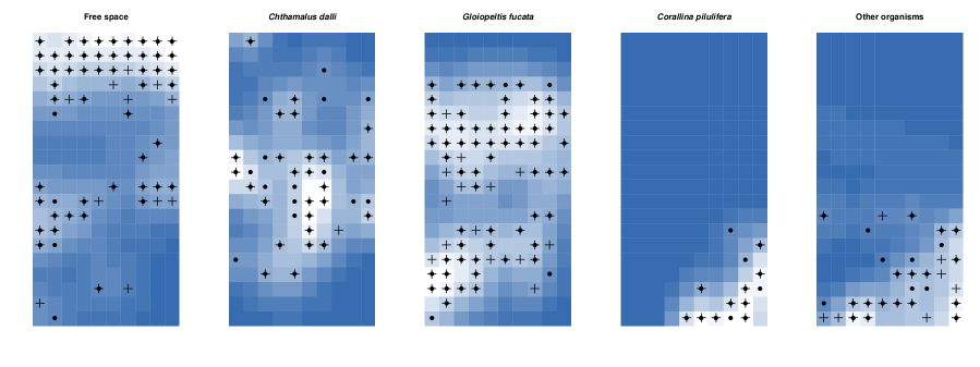
Figure 3: Observed data, occupancy, and local state dominance for a particular quadrat (MC2) and point in time estimated using the spatial model, mapped on the spatial coordinates of each observation point (20 horizontal rows $\times$ 10 vertical columns). Filled circles ($\bullet$) and crosses ($+$) represent data (the state observed at each observation point) and estimated site occupancy state (the state that had the highest posterior probability of occupancy at each observation point), respectively. Note that for each site, both filled circles and crosses appear in only one of the five panels, which represent different ecological states. The estimated local state dominance, $g_{its}$, is represented by colored squares. A brighter square indicates greater dominance of the state at that location.

DISCUSSION

In this study, we proposed a multistate dynamic site occupancy model for aggregated sessile communities. The model accounts for the resampling error that is associated with local community structure. The model assumes underlying surfaces of local dominance for each of the possible ecological states that determines the distribution of data that are conditional on the occurrence of the resampling error. The surface is estimated nonparametrically by using a multivariate kernel smoothing method, in which the local species dominance at an arbitrary location is obtained as a function of the underlying occupancy of states across all sites.

In ecological studies, consideration of spatial effects has been thought to be fundamental (Legendre 1993, Lichstein et al. 2002, Royle et al. 2007). It has also been widely recognized that accounting for observation processes in data collection and analyses is important because ignoring these processes may lead to biased estimates and thus misleading conclusions (Williams et al. 2002, Kéry and Schaub 2012, Kéry and Royle 2016). These two considerations have been incorporated into the dynamic site occupancy modeling framework to study metapopulation dynamics while accounting for imperfect detection (e.g., Bled et al. 2011, Risk et al. 2011, Yackulic et al. 2012). As far as we know, however, such spatial dynamic site occupancy models have been applied only to population dynamics of single species (but see Yackulic et al. (2014)). The spatial multistate dynamic site occupancy model we developed here would be widely applicable to studying the dynamics of sessile communities in various systems, including corals, mussels and terrestrial plants, for which precise resampling of observation points may be difficult in the field for practical reasons (Conway-Cranos and Doak 2011).

For spatially referenced site occupancy data, dynamic site occupancy models with autologistic components have been proposed (Bled et al. 2011, 2013, Yackulic et al. 2012, 2014, Eaton et al. 2014 ; see also Broms et al. 2016). In these models, the adjacency of sites must be defined a priori, because probabilities of occupancy, local colonization and extinction are assumed to depend on the occupancy states of neighboring sites. It has also been typical in the application of these models that sites are aligned on grids. However, as has been done in this study, another approach for modeling spatial effects is to use kernel-weighting functions. Several dynamic site occupancy models that were recently developed based on the metapopulation theory use this approach to account for spatial dependency of local colonization and extinction probabilities (Risk et al. 2011, Heard et al. 2013, Sutherland et al. 2014, Chandler et al. 2015). Because the scale of correlation is determined by the data, this modeling approach does not require a priori determination of site adjacency. The observation sites may also not need to be aligned in a reticular pattern. A related weighting function approach has also been used to identify the spatial scale at which landscape variables affect abundance (Chandler and Hepinstall-Cymerman 2016). We note, however, that a possible difficulty in using kernel weighting may be its associated computational burden. Evaluating the kernel weights for every combination of two sites may be time-consuming, and the amount of computation time required increases very rapidly with the number of sites being considered.

The multivariate Gaussian kernel used in the proposed model can account for an anisotropic spatial correlation of community structure. This characteristic of the multivariate Gaussian kernel can be useful when a known, or even unknown, environmental gradient exists in the quadrat and affects the distribution of sessile species. Although other types of kernels may be used to model the spatial structure, the multivariate Gaussian kernel allows a straightforward implementation of anisotropic correlation by specifying a bandwidth matrix with scale and correlation parameters. However, results of our simulation study suggest that, in the proposed model, bandwidth parameters may be difficult to estimate when the resampling error rate is quite low. In such cases, the proposed spatial model would not be a reasonable option for the inference of transition probabilities. In this regard, adoption of a robust design is recommended because obtaining replicated samples may mitigate this problem (Fig. 1). We note that dynamic occupancy models in general do not require equal numbers of replications for every site and time.

Results from a dataset of intertidal communities on the Pacific coast of eastern Hokkaido highlight the fact that different models may produce considerably different estimates of transition probabilities as well as of the properties of community dynamics, which are obtained from the transition probability matrix (Table 1, Fig. 2). We have shown that, compared to the non-spatial model (Fukaya and Royle 2013), the spatial model tends to yield a higher persistence probability of each state, longer mean turnover time and lower damping ratio. These differences were even greater when the spatial model was compared to the naive model. In the assessment of their intertidal sessile community data from California, Conway-Cranos and Doak (2011) also found that the estimated damping ratio was higher when resampling errors were not corrected. These results have implications for the development of management plans that are based on Markovian models. They suggest that ignoring the existence of resampling errors, as well as local community structure, may lead to overestimation of the recovery rate of ecological communities from natural or anthropogenic disturbance, the result being poorly informed management strategies.

The hierarchical formulation of the model allows us to readily extend the proposed model, at least conceptually, to add more ecological realism (Royle and Dorazio 2008, Kéry and Schaub 2012, Kéry and Royle 2016). For example, if some site- or time-specific environmental covariates are available, they may be incorporated into the model to take account of variations in transition probabilities and error rates. A possible extension of the model that may have a particular ecological significance is to link estimated local state dominance $g_{its}$ values to transition probabilities. Because interactions between sessile organisms are limited to neighboring individuals, the rate of local colonization, persistence, and replacement are expected to depend on surrounding local community structure (Wootton 2001a, Kawai and Tokeshi 2006). Although the dependency of transition probabilities on species frequency has been considered in previous studies about Markovian community dynamics (i.e., nonlinear Markov community model; Spencer and Tanner 2008, Tanner et al. 2009), only the connection between transition probabilities and the overall (i.e., global) species frequency has been explored. However, by using the underlying occupancy component explicitly, dynamic site occupancy models can model a relationship between local occupancy density and the rates of colonization and/or extinction (Bled et al. 2011, Risk et al. 2011, Yackulic et al. 2012), although such dependency has rarely been modeled in a multispecies context (but see Yackulic et al. (2014) who explored intra- and inter-specific effects on site occupancy dynamics of two owl species). Because the proposed model explicitly involves local community structure as a model component, it will naturally provide a basis for inferring complex nonlinear ecological dynamics.

Appendix A JAGS model code

model {
    ## Observation model
    for (i in 1:I) {
        for (t in 1:T) {
            for (n in 1:N[i, t]) {
                # m: indicator for resampling error, 1 represents resampling error
                m[i, t, n] ~ dbern(e)
                for (s in 1:S) {
                    # q: observation probabilities (conditional on m)
                    q[i, t, n, s] <- ((1 - m[i, t, n]) * equals(z[i, t], s)
                        + m[i, t, n] * g[i, t, s])
                }
                # y: observed data
                y[i, t, n] ~ dcat(q[i, t, n, ])
            }
        }
    }

    ## Process model
    for (i in 1:I) {
        # z: occupancy state
        z[i, 1] ~ dcat(phi[])
        for (t in 2:T) {
            z[i, t] ~ dcat(p[, z[i, t - 1]])
        }
    }

    ## Kernel estimator
    # Sigma: bandwidth matrix
    Sigma[1, 1] <- sigma1^2
    Sigma[1, 2] <- rho * sigma1 * sigma2
    Sigma[2, 1] <- rho * sigma1 * sigma2
    Sigma[2, 2] <- sigma2^2

    # V: inverse of the bandwidth matrix
    V <- inverse(Sigma)

    for (i in 1:I) {
        for (j in 1:I) {
            # K: weight matrix
            K[i, j] <- exp(- vd[i, j, ] %*% V %*% vd[i, j, ] / 2)
        }
    }

    for (i in 1:(I - 1)) {
        # dS: Diagonal matrix of the inverse sum of weights
        dS[i, i] <- 1 / sum(K[i, ])
        for (j in (i + 1):I) {
            dS[i, j] <- 0
            dS[j, i] <- 0
        }
    }
    dS[I, I] <- 1 / sum(K[I, ])

    for (t in 1:T) {
        # mz: array of indicator of occupancy state
        for (s in 1:S) {
            mz[1:I, t, s] <- equals(z[, t], s)
        }
        # g: relative state dominance
        g[1:I, t, 1:S] <- dS %*% K %*% mz[, t, ]
    }

    ## Priors
    # e: resampling error rate
    e ~ dbeta(1, 1)

    # P: transition probabilities
    for (s in 1:S) {
        p[1:S, s] ~ ddirch(alpha)
    }

    # phi: initial occupancy probabilities
    phi[1:S] ~ ddirch(alpha)

    # sigma: scale parameter of the Gaussian kernel
    sigma1 ~ dunif(0, U)
    sigma2 ~ dunif(0, U)

    # rho: correlation parameter of the Gaussian kernel
    rho ~ dunif(-1, 1)
}

LITERATURE CITED

- Benedetti-Cecchi (2001) Benedetti-Cecchi, L., 2001. Variability in abundance of algae and invertebrates at different spatial scales on rocky sea shores. Marine Ecology Progress Series 215:79–92.
- Bled et al. (2013) Bled, F., J. D. Nichols, and R. Altwegg, 2013. Dynamic occupancy models for analyzing species’ range dynamics across large geographic scales. Ecology and Evolution 3:4896–4909.
- Bled et al. (2011) Bled, F., J. A. Royle, and E. Cam, 2011. Hierarchical modeling of an invasive spread: the Eurasian Collared-Dove Streptopelia decaocto in the United States. Ecological Applications 21:290–302.
- Broms et al. (2016) Broms, K. M., M. B. Hooten, D. S. Johnson, R. Altwegg, and L. L. Conquest, 2016. Dynamic occupancy models for explicit colonization processes. Ecology 97:194–204.
- Chandler and Hepinstall-Cymerman (2016) Chandler, R. and J. Hepinstall-Cymerman, 2016. Estimating the spatial scales of landscape effects on abundance. Landscape Ecology (in press).
- Chandler et al. (2015) Chandler, R. B., E. Muths, B. H. Sigafus, C. R. Schwalbe, C. J. Jarchow, and B. R. Hossack, 2015. Spatial occupancy models for predicting metapopulation dynamics and viability following reintroduction. Journal of Applied Ecology 52:1325–1333.
- Conway-Cranos and Doak (2011) Conway-Cranos, L. L. and D. F. Doak, 2011. Sampling errors create bias in Markov models for community dynamics: the problem and a method for its solution. Oecologia 167:199–207.
- Diggle et al. (2005) Diggle, P., P. Zheng, and P. Durr, 2005. Nonparametric estimation of spatial segregation in a multivariate point process: bovine tuberculosis in Cornwall, UK. Journal of the Royal Statistical Society: Series C (Applied Statistics) 54:645–658.
- Eaton et al. (2014) Eaton, M. J., P. T. Hughes, J. E. Hines, and J. D. Nichols, 2014. Testing metapopulation concepts: effects of patch characteristics and neighborhood occupancy on the dynamics of an endangered lagomorph. Oikos 123:662–676.
- Fukaya et al. (2014) Fukaya, K., T. Okuda, M. Nakaoka, and T. Noda, 2014. Effects of spatial structure of population size on the population dynamics of barnacles across their elevational range. Journal of Animal Ecology 83:1334–1343.
- Fukaya and Royle (2013) Fukaya, K. and J. A. Royle, 2013. Markov models for community dynamics allowing for observation error. Ecology 94:2670–2677.
- Gelman et al. (2014) Gelman, A., J. B. Carlin, H. S. Stern, D. B. Dunson, A. Vehtari, and D. B. Rubin, 2014. Bayesian Data Analysis. Taylor & Francis, third edition.
- Ghahramani and Jordan (1997) Ghahramani, Z. and M. I. Jordan, 1997. Factorial hidden Markov models. Machine learning 29:245–273.
- Heard et al. (2013) Heard, G. W., M. A. McCarthy, M. P. Scroggie, J. B. Baumgartner, and K. M. Parris, 2013. A bayesian model of metapopulation viability, with application to an endangered amphibian. Diversity and Distributions 19:555–566.
- Hill et al. (2002) Hill, M. F., J. D. Witman, and H. Caswell, 2002. Spatio-temporal variation in Markov chain models of subtidal community succession. Ecology Letters 5:665–675.
- Hill et al. (2004) Hill, M. F., J. D. Witman, and H. Caswell, 2004. Markov chain analysis of succession in a rocky subtidal community. American Naturalist 164:E46–61.
- Kawai and Tokeshi (2006) Kawai, T. and M. Tokeshi, 2006. Asymmetric coexistence: bidirectional abiotic and biotic effects between goose barnacles and mussels. Journal of Animal Ecology 75:928–941.
- Kéry and Royle (2016) Kéry, M. and J. A. Royle, 2016. Applied Hierarchical Modeling in Ecology: Analysis of Distribution, Abundance and Species Richness in R and BUGS. Volume 1: Prelude and Static Models. Academic Press.
- Kéry and Schaub (2012) Kéry, M. and M. Schaub, 2012. Bayesian Population Analysis using WinBUGS: A Hierarchical Perspective. Academic Press.
- Legendre (1993) Legendre, P., 1993. Spatial autocorrelation: trouble or new paradigm? Ecology 74:1659–1673.
- Lichstein et al. (2002) Lichstein, J. W., T. R. Simons, S. A. Shriner, and K. E. Franzreb, 2002. Spatial autocorrelation and autoregressive models in ecology. Ecological Monographs 72:445–463.
- Nakaoka et al. (2006) Nakaoka, M., N. Ito, T. Yamamoto, T. Okuda, and T. Noda, 2006. Similarity of rocky intertidal assemblages along the Pacific coast of Japan: effects of spatial scales and geographic distance. Ecological Research 21:425–435.
- Okuda et al. (2004) Okuda, T., T. Noda, T. Yamamoto, N. Ito, and M. Nakaoka, 2004. Latitudinal gradient of species diversity: multi-scale variability in rocky intertidal sessile assemblages along the Northwestern Pacific coast. Population Ecology 46:159–170.
- Plummer (2003) Plummer, M., 2003. JAGS: A program for analysis of Bayesian graphical models using Gibbs sampling. In Proceedings of the 3rd international workshop on distributed statistical computing (DSC 2003), volume 124, page 125. Technische Universit at Wien, Austria.
- Pollock (1982) Pollock, K. H., 1982. A capture-recapture design robust to unequal probability of capture. Journal of Wildlife Management 46:752–757.
- Risk et al. (2011) Risk, B. B., P. de Valpine, and S. R. Beissinger, 2011. A robust-design formulation of the incidence function model of metapopulation dynamics applied to two species of rails. Ecology 92:462–474.
- Royle and Dorazio (2008) Royle, J. A. and R. M. Dorazio, 2008. Hierarchical Modeling and Inference in Ecology: the Analysis of Data from Populations, Metapopulations and Communities. Academic Press.
- Royle et al. (2007) Royle, J. A., M. Kéry, R. Gautier, and H. Schmid, 2007. Hierarchical spatial models of abundance and occurrence from imperfect survey data. Ecological Monographs 77:465–481.
- Spencer and Susko (2005) Spencer, M. and E. Susko, 2005. Continuous-time Markov models for species interactions. Ecology 86:3272–3278.
- Spencer and Tanner (2008) Spencer, M. and J. E. Tanner, 2008. Lotka-Volterra competition models for sessile organisms. Ecology 89:1134–1143.
- Sutherland et al. (2014) Sutherland, C. S., D. A. Elston, and X. Lambin, 2014. A demographic, spatially explicit patch occupancy model of metapopulation dynamics and persistence. Ecology 95:3149–3160.
- Tanner et al. (2009) Tanner, J. E., T. P. Hughes, and J. H. Connell, 2009. Community-level density dependence: an example from a shallow coral assemblage. Ecology 90:506–516.
- Valdivia et al. (2011) Valdivia, N., R. A. Scrosati, M. Molis, and A. S. Knox, 2011. Variation in community structure across vertical intertidal stress gradients: how does it compare with horizontal variation at different scales? PLoS ONE 6:e24062.
- Williams et al. (2002) Williams, B. K., J. D. Nichols, and M. J. Conroy, 2002. Analysis and Management of Animal Populations. Academic Press.
- Wootton (2001a) Wootton, J. T., 2001a. Local interactions predict large-scale pattern in empirically derived cellular automata. Nature 413:841–844.
- Wootton (2001b) Wootton, J. T., 2001b. Prediction in complex communities: analysis of empirically derived Markov models. Ecology 82:580–598.
- Yackulic et al. (2012) Yackulic, C. B., J. Reid, R. Davis, J. E. Hines, J. D. Nichols, and E. Forsman, 2012. Neighborhood and habitat effects on vital rates: expansion of the Barred Owl in the Oregon Coast Ranges. Ecology 93:1953–1966.
- Yackulic et al. (2014) Yackulic, C. B., J. Reid, J. D. Nichols, J. E. Hines, R. Davis, and E. Forsman, 2014. The roles of competition and habitat in the dynamics of populations and species distributions. Ecology 95:265–279.