Completeness of Inertial Modes of an Incompressible Inviscid Fluid in a Corotating Ellipsoid

Abstract

Inertial modes are the eigenmodes of contained rotating fluids restored by the Coriolis force. When the fluid is incompressible, inviscid and contained in a rigid container, these modes satisfy Poincaré’s equation that has the peculiarity of being hyperbolic with boundary conditions. Inertial modes are therefore solutions of an ill-posed boundary-value problem. In this paper we investigate the mathematical side of this problem. We first show that the Poincaré problem can be formulated in the Hilbert space of square-integrable functions, with no hypothesis on the continuity or the differentiability of velocity fields. We observe that with this formulation, the Poincaré operator is bounded and self-adjoint and as such, its spectrum is the union of the point spectrum (the set of eigenvalues) and the continuous spectrum only. When the fluid volume is an ellipsoid, we show that the inertial modes form a complete base of polynomial velocity fields for the square-integrable velocity fields defined over the ellipsoid and meeting the boundary conditions. If the ellipsoid is axisymmetric then the base can be identified with the set of Poincaré modes, first obtained by Bryan (1889) Bryan (1889), and completed with the geostrophic modes.

I Introduction

Rotation is a ubiquitous feature in stars, planets and satellites. The dynamics of these objects is profoundly modified when solid body rotation overwhelmingly dominates all other flows. In this case residual disturbances that make the flow depart from an exact solid body rotation are strongly affected by the Coriolis acceleration which ensures angular momentum conservation of the movements. This is especially true for the low frequency oscillations of stars or planets. For these oscillations buoyancy and Coriolis force are the restoring forces at work. They make gravito-inertial waves possible Friedlander and Siegmann (1982); Dintrans et al. (1999).

In stars these waves are of strong interest because their detection and identification allow us to access to both the Brunt-Väisälä frequency distribution as well as the local rotation of the fluid. They are of particular interest in massive stars, where they open a window on the interface separating the inner convective core and the outer radiative, and stably stratified, envelope. But these waves are also a key feature of the response of tidally interacting bodies and therefore of their secular evolution Ogilvie and Lin (2004); Ogilvie (2005); Rieutord and Valdettaro (2010); Ogilvie (2014). On this latter subject several studies have recently addressed the dynamics of fluid flows driven by librations, which are common phenomena in planetary satellites (e.g. Sauret and Le Dizès, 2013; Zhang et al., 2012, 2013).

However, the mathematical problem set out by these global oscillations is far from being fully understood. The reason for that comes from the very basic boundary value problem that emerges when diffusion and compressibility effects are neglected: it is ill-posed mathematically Greenspan (1968). The operator is indeed either of hyperbolic or mixed type in the spatial coordinates, but the solutions need to match boundary conditions. As already noted by many authors after the seminal work of Hadamard Hadamard (1932), ill-posed problems are plagued with many sorts of singularities (e.g. Rieutord et al., 2001, for a detailed discussion).

With planetary and stellar applications in mind the oscillations of an incompressible fluid confined in a rotating sphere or spherical shell have attracted much attention Hollerbach and Kerswell (1995); Rieutord and Valdettaro (1997); Rieutord et al. (2000, 2001); Rieutord and Valdettaro (2010); Sauret and Le Dizès (2013). The oscillating flows in a spherical shell display strong singularities when viscosity vanishes Rieutord et al. (2001). The singularities occur because perturbations obey the spatially hyperbolic Poincaré equation (see Eq 9b below), and must meet boundary conditions. The strongest singularities, called wave attractors after the work of Maas & Lam Maas and Lam (1995), result from the reflection of the characteristic lines (or surfaces) on the boundaries. In the two-dimensional problem analog to that of the spherical shell, characteristic lines are focussing around periodic orbits (the attractors) Rieutord et al. (2002). It can be further shown that no eigenmode can exist when an attractor is present Rieutord et al. (2001). Of course viscosity regularizes the solutions, but numerical solutions of the viscous eigenvalue problem show that actual eigenmodes are strongly featured by attractors. They appear as thin oscillating shear layers attached to the attractor.

Surprisingly, when the inner core of the spherical shell is suppressed, namely the container is a full sphere (or a full ellipsoid) regular polynomial solutions exist for the inviscid eigenvalue problem Vantieghem (2014). For the sphere and the axisymmetric ellipsoid, these solutions have long been known since the paper of Bryan Bryan (1889), which followed the seminal work of Poincaré Poincaré (1885) on the equilibrium of rotating fluid masses (but see also Greenspan, 1968; Zhang et al., 2001).

When Greenspan Greenspan (1968) reviewed the subject in his monograph on rotating fluids, he raised the question of the completeness of the inertial modes in the sphere and the ellipsoid. Indeed, if the normal modes are complete, then any perturbation can be expanded into a linear combination of eigenfunctions. In particular any initial condition can be expanded and the response flow can be calculated, while perturbations by viscous or nonlinear effects can be easily dealt with. Except for the work of Lebovitz Lebovitz (1989) (see below), Greenspan’s question remained untouched for almost fifty years until the recent works of Cui et al. Cui et al. (2014), who proved completeness for the rotating annular channel, followed by the one of Ivers et al. Ivers et al. (2015) who gave the demonstration for the sphere.

The present work, which has an unusual history (see the end of the paper), extends the results of Ivers et al. to any ellipsoid. Importantly, our demonstration takes another route than the one found by Ivers et al.Ivers et al. (2015). We use a more general formulation of the problem allowing us to use the tools of functional analysis in the Hilbert space of square-integrable functions. Since these tools are likely unfamilar to many fluid dynamicists, we try to make our demonstration as pedagogical as possible.

The paper is organised as follows. In the next section we first formulate the Poincaré problem, either for forced flows or for free oscillations. Then, in section 3, we propose another formulation of the free oscillation problem that does not assume continuity or differentiability of velocity fields. Velocity fields are only supposed to be square-integrable. Such an extension of the space of velocity fields is motivated by three arguments: first, inviscid fluid may support discontinuous velocity fields, like the classical vortex sheet Rieutord (2015). Second, singular velocity field can be expected because of the ill-posed nature of the Poincaré problem. Third, and not least, by assuming only square-integrability of the solution of the problem, we can play in the Hilbert space of square-integrable functions, and benefit from many results of spectral theory on bounded, self-adjoint, linear operators. In section 4, we summarize what we can readily say about this problem using some of the results of functional analysis, recalling in passing the needed concepts of spectral analysis. We then establish a sufficient condition for an operator to own a complete basis of eigenfunctions. We show that polynomial eigenfunctions can constitute such a base if the fluid volume is an ellipsoid. This result was also obtained by Lebovitz Lebovitz (1989), but our proof is more direct and clearly exhibit the special nature of the ellipsoidal boundary. In section 5, we consider the well-known (since Bryan 1889) eigenmodes of the rotating spheroid (i.e. the axisymmetric ellipsoid). These solutions are of polynomial nature and we show (section 6) that they constitute the expected complete base that has been infered in the previous section. Notably, we exhibit the set of geostrophic modes that are associated with the zero-eigenfrequency, and without which inertial modes would not make a complete base.

The present work is therefore a follow up of the work of Ivers et al. Ivers et al. (2015) who obtained a first set of mathematical results when the problem is restricted to the sphere and when the velocity fields are supposed to be once-continuously differentiable. The two works share many common results, but hopefully they complete one another and offer the broadest view of the Poincaré problem. The method proposed here seems promising enough that one might hope to use it when the fluid volume is not an ellipsoid. We have investigated two other shapes, a cube and a spherical shell, with only negative results. Hence, except the annular channel Cui et al. (2014), we simply do not know whether any non-ellipsoidal volume has a complete set of eigenvelocities of some more general form.

II Classical Formulation of the Poincaré problem

In the steady, undisturbed reference state, an incompressible non-viscous fluid with constant density $\rho$ occupies an open bounded set $E$ with boundary $\partial E$ that has an outward unit normal ${\hat{\bf n}}$. Let $\overline{E}$ be the closure of $E$, i.e. $E$ together with $\partial E$. Both $\partial E$ and the fluid rotate rigidly about some given axis with constant angular velocity ${\bf\Omega}$. Position vectors ${\bf r}$ are measured relative to an origin chosen on the axis of rotation. The body force on the fluid in the rotating reference frame is independent of time and consists of self-gravity, externally applied gravity, and centrifugal force. The pressure in the fluid is the hydrostatic pressure required to balance these body forces.

In the disturbed state $\partial E$ is infinitesimally deformed to $\partial E_{t}$ at time $t$, and the infinitesimal normal velocity of $\partial E_{t}$ is $\beta$. An extra infinitesimal time-dependent body force ${\bf f}$ per unit mass acts on the fluid. In consequence of these forces and its own history, the fluid has an infinitesimal velocity ${\bf v}$ when viewed from the rotating frame. The hydrostatic pressure suffers an infinitesimal perturbation which it will be convenient to write as $2\rho\Omega q$, where $\Omega$ is the magnitude of ${\bf\Omega}$ and $q$ is a function of ${\bf r}$ and the time $t$. In the rotating reference frame, ${\bf v}$ and q are governed by the equations

$${\hat{\bf n}}\,\cdot\,{\bf v}\ =\ \beta\qquad{\rm on}\quad\partial E,$$ (1a)

$$\nabla\cdot{\bf v}\ =\ 0\qquad{\rm in}\quad E,$$ (1b)

$$\partial_{t}{\bf v}\ +\ 2\,{\bf\Omega}\,\times{\bf v}\ =\ -2\Omega\nabla q\ +\ {\bf f}\ \ \ \ \ \ {\rm in}\ \ \ E.$$ (2)

Because $\rho$ is constant, (1b) is exact, but (1a) and (2) are correct only to first order in the disturbances $\beta$, ${\bf v}$, $q$ and ${\bf f}$. For simplicity it will be assumed that $\beta$ and ${\bf f}$ are known for all $t>0$, and that ${\bf v}$ is known everywhere at $t\ =\ 0$. Using this information to find ${\bf v}$ and $q$ for all ${\bf r}$ in $E$ and all $t>0$ constitutes the Poincaré forced initial value problem.

It will be convenient to eliminate $\beta$ at the outset. If $\beta\neq 0$, let $\theta$ be a solution of the following Neumann problem (Kellogg, 1953, p246) at each time $t$ :

$${\hat{\bf n}}\,\cdot\,\nabla\theta\ =\ \beta\qquad{\rm on}\ \ \ \partial E,$$ (3a)

$$\nabla^{2}\,\theta\ =\ 0\qquad{\rm in}\ \ \ E.$$ (3b)

The solubility conditions for this Neumann problem are that $\partial E$ be sufficiently smooth (for example, $\hat{\bf n}$ may vary continuously on $\partial E$) and that

$$\int_{\partial E}\,dA\ \beta\ =\ 0,$$ (3c)

a condition whose fulfillment is assured by (1b). Given (3c), the solution $\theta$ of (3a,b) is determined at each $t$ up to an unknown additive function of $t$, and $\nabla\theta$ is uniquely determined for all $t$. If we define

$${\bf v}^{\prime}\ =\ {\bf v}\ -\ \nabla\theta$$ (4a)

then $${\bf v}^{\prime} \beta q$$ satisfies equations (1b) and (2) with replaced by 0, with replaced by

$$q^{\prime}\ =\ q\ +\ (2\Omega)^{-1}\ \partial_{t}\theta$$ (4b)

and with ${\bf f}$ replaced by

$${\bf f}^{\prime}\ =\ {\bf f}\ -\ 2{\bf\Omega}\ \times\ \nabla\theta.$$ (4c)

Henceforth we drop the primes and take $\beta\ =\ 0$ in (1a).

To find the normal modes we set ${\bf f}\ =\ {\bf 0}$ in (2) and look for solutions of (1b) and (2) whose time dependence is

$${\bf v}({\bf r},t)\ =\ {\bf v}({\bf r},0)\ e^{{2i}\Omega\lambda t}$$ (5a)

$$q({\bf r},t)\ =\ q({\bf r},0)\ e^{{2i}\Omega\lambda t}$$ (5b)

where $\lambda$ is an unknown complex constant. In studying the normal modes we will abbreviate ${\bf v}({\bf r},0)$ and $q({\bf r},0)$ as ${\bf v}({\bf r})$ and $q({\bf r})$ or simply as ${\bf v}$ and $q$. In these circumstances, (1b) and (2) are replaced by

$${\hat{\bf n}}\,\cdot\,{\bf v}\ =\ 0\qquad{\rm on}\quad\partial E,$$ (6a)

$$\nabla\,\cdot\,{\bf v}\ =\ 0\qquad{\rm in}\quad E,$$ (6b)

$$-\lambda{\bf v}\ +\ i\,{\hat{\bf\Omega}}\,\times{\bf v}\ =\ -i\,\nabla q\qquad{\rm in}\quad E,$$ (7)

where ${\hat{\bf\Omega}}\ =\ {\bf\Omega}/\Omega$, the unit vector in the direction of ${\bf\Omega}$.

Kudlick (1966) Kudlick (1966) and Greenspan (1968) show that when ${\bf v}$ and $q$ are smooth enough to permit some differentiation then $\lambda$ cannot be $+1$ or $-1$. We will treat the geostrophic case ($\lambda\ =\ 0$) later, so for the moment we assume that $\lambda$ is not 0, +1 or $-1$. Then (Greenspan, 1968, p.51) equation (7) can be solved for ${\bf v}$ in terms of $\nabla q$ to produce

$$\lambda(1\,-\,\lambda^{2})\,{\bf v}\ =\ -i\,\lambda^{2}\,\nabla q\ +\ \lambda\,{\hat{\bf\Omega}}\,\times\,\nabla q\ +\ i\,\hat{\bf\Omega}\;{\hat{\bf\Omega}}\cdot\nabla q\;.$$ (8)

Substituting (8) in (6a) gives

$$\lambda^{2}\,{\hat{\bf n}}\,\cdot\,\nabla q\ +\ i\lambda({\hat{\bf n}}\,\times\,{\hat{\bf\Omega}})\,\cdot\,\nabla q\ =\ ({\hat{\bf n}}\,\cdot\,{\hat{\bf\Omega}})\,({\hat{\bf\Omega}}\,\cdot\,\nabla q)\ \ \ \ \ \ {\rm on}\ \ \ \partial E.$$ (9a)

Substituting (8) in (6b) gives

$$({\hat{\bf\Omega}}\,\cdot\,\nabla)^{2}\,q\ =\ \lambda^{2}\,\nabla^{2}\,q\qquad{\rm in}\quad E.$$ (9b)

Equation (9b) is the classical Poincaré equation for the pressure disturbance $q$, and (9a) is the boundary condition appropriate to the Poincaré problem, in which $\partial E$ rotates rigidly. Given an eigenfunction $q$ and its eigenvalue $\lambda$ in (9b), the corresponding ${\bf v}$ is recovered from (8). Greenspan (1965) Greenspan (1965) shows that when ${\bf v}$ is sufficiently differentiable then $\lambda$ must be real and between $-1$ and 1. The resulting hyperbolic character of (9b) for the normal modes has led to the suspicion that there might be pathological elements in the boundary value problem (9b) Stewartson and Rickard (1969).

III Admitting non-differentiable velocity fields

III.1 Introduction

Inviscid incompressible fluids admit discontinuous velocity fields provided discontinuities are parallel to the field so as to fulfill mass conservation. Hence, eigenvalues may be associated with non-differentiable velocity fields. In view of the ill-posed nature of the Poincaré problem, the possibility of such eigen-velocities cannot be excluded. In this section we therefore reformulate the eigenvalue problem (6b)-(7) in order to include non-differentiable velocity fields.

Under suitable smoothness assumptions Greenspan (1964, 1965) Greenspan (1964, 1965) shows that, whatever the shape of the fluid volume $E$, all eigenvalues $\lambda$ of (6b) and (7) are real and lie in the interval $-1<\lambda<1$. That author also shows that eigenvelocities $\,{\bf v}_{1}$ and $\,{\bf v}_{2}$ belonging to different eigenvalues $\lambda_{1}$ and $\lambda_{2}$ are orthogonal in the sense that $\langle\ {\bf v}_{1}\,|\,{\bf v}_{2}\,\rangle\ =\ 0$, where the inner product is defined as

$$\langle\ {\bf v}_{1}\,|\,{\bf v}_{2}\,\rangle\ =\ |E|^{-1}\ \int_{E}\,dV({\bf r})\ {\bf v}_{1}({\bf r})^{*}\cdot\,{\bf v}_{2}({\bf r})\;.$$ (10)

Here $|E|$ is the volume of the region $E$, and ${\bf v}_{1}({\bf r})^{*}$ is the complex conjugate of ${\bf v}_{1}({\bf r})$.

All this suggests that the eigenvalues $\lambda$ are the eigenvalues of some bounded, self-adjoint linear operator $L$ on the complex Hilbert space $\underline{\bf\Pi}$ consisting of all Lebesgue square-integrable complex vector fields ${\bf v}$ on $E$. We recall that square-integrability just means that the total kinetic energy of the flow exists. For such velocity fields, we can define their norm by

$$\|{\bf v}\|\ =\ \langle\ {\bf v}\,|\,{\bf v}\,\rangle\,^{{1\over 2}}\,.$$ (11)

Now, to find the appropriate operator $L\,:\,\underline{\bf\Pi}\ \to\ \underline{\bf\Pi}$, we must interpret (6b) and (7) when ${\bf v}$ is merely square-integrable and not differentiable or even continuous.

III.2 Mass conservation for $\mbox{${\cal L}$}^{2}$-velocity fields

For velocity fields ${\bf v}$ that are merely square-integrable and not differentiable or even continuous $\nabla\cdot\,{\bf v}$ is not well-defined in $E$, and $\hat{\bf n}\,\cdot\,{\bf v}$ is not well-defined on $\partial E$. We begin by trying to avoid this difficulty.

The game will be to define subspaces of the general Hilbert space $\underline{\bf\Pi}$ that includes all the square-integrable complex vector fields ${\bf v}$ defined on $E$. To ease reading, we shall use underlined symbols to denote a space (of functions usually). It’ll be boldface if the space is a space of vectorial functions. Thus, we first introduce $\underline{\Pi}^{\infty}$ and $\underline{\bf\Pi}^{\infty}$ that are respectively the spaces of all infinitely differentiable complex scalar and vector fields on $\overline{E}$, the closure of $E$. Define

$$\underline{\bf\Gamma}^{\infty}:=\nabla\Pi^{\infty}\,.$$ (12a)

That is, $$\underline{\bf\Gamma}\,^{\infty} {\bf u}$$ consists of all vector fields which can be written

$${\bf u}\ =\ \nabla\,\phi$$ (12b)

for some $\phi$ in $\Pi^{\infty}$. Then clearly $\underline{\bf\Gamma}^{\infty}\,\subseteq\,\underline{\bf\Pi}$, but $\underline{\bf\Gamma}\,^{\infty}$ is not closed in $\underline{\bf\Pi}$ under the norm (11). Indeed, we can easily construct a suite of infinitly differentiable function that converges to a discontinuous function. Therefore, we consider its closure, $\underline{\bf\Gamma}$:

$$\underline{\bf\Gamma}:=\overline{\underline{\bf\Gamma}^{\infty}}\,.$$ (13)

According to this definition, a vector field ${\bf u}$ on $E$ belongs to $\underline{\bf\Gamma}$ if and only if it is square-integrable on $E$ and there is a sequence $\phi_{1},\ \phi_{2},\,...$ in $\underline{\Pi}^{\infty}$ such that

$$\lim_{n\to\infty}\|{\bf u}-\nabla\phi_{n}\|=0\,.$$ (14)

In particular, $\underline{\bf\Gamma}$ includes all fields ${\bf u}$ of form (12b) with $\phi$ continuously differentiable on $\overline{E}$.

Let us now introduce $\underline{\bf\Lambda}$, the orthogonal complement of $\underline{\bf\Gamma}$ in $\underline{\bf\Pi}$. Thus $\underline{\bf\Lambda}$ consists of all vector fields ${\bf w}$ square-integrable on $E$ and such that $\langle\,{\bf u}|{\bf w}\,\rangle=0$ for every ${\bf u}$ in $\underline{\bf\Gamma}$. In particular, ${\bf w}\in\underline{\bf\Lambda}$ implies that

$$|E|^{-1}\ \int_{E}\,dV({\bf r})\ (\nabla\phi^{*})\cdot{\bf w}\ =\ 0$$ (15)

for every $\phi$ in $\underline{\Pi}^{\infty}$. Conversely, since the orthogonal complement of a set is also the orthogonal complement of its closure, if ${\bf w}$ is square-integrable on $E$ and (15) is true for every $\phi$ in $\underline{\Pi}^{\infty}$, then ${\bf w}\in\underline{\bf\Lambda}$.

Now suppose ${\bf w}\in\underline{\bf\Lambda}\cap\underline{\bf\Pi}^{\infty}$. Then, Gauss’s theorem permits (15) to be rewritten as

$$\int_{\partial E}dA\phi^{*}(\hat{\bf n}\cdot{\bf w})-\int_{E}dV\phi^{*}(\nabla\cdot{\bf w})=0\quad\forall\phi\in\underline{\Pi}^{\infty}\,.$$ (16)

By the Weierstrass approximation theorem (Courant and Hilbert, 1953, p65) every $\phi$ continuous on $\overline{E}$ can be approximated uniformly and with arbitrary accuracy by polynomials. Therefore (16) holds for all $\phi$ continuous on $\overline{E}$. Then a well-known argument leads to the conclusion that $\nabla\,\cdot\,{\bf w}\,=\,0$ in $E$ and ${\hat{\bf n}}\,\cdot\,{\bf w}\,=\,0$ on $\partial E$. Therefore, the demand

$${\bf v}\in\underline{\bf\Lambda}$$ (17)

is the appropriate generalization of (6b) to square-integrable vector fields which are not differentiable.

III.3 $\underline{\bf\Lambda}$ and piecewise continuously differentiable fields

Before going any further, it is worth viewing (17) from a physical point of view. $\underline{\bf\Lambda}$ is indeed a very large space that includes, among other fields, unbounded vector fields that are not physically acceptable.

We know that the local equation $\nabla\cdot\mathbf{v}=0$ is equivalent to the integral condition

$$\int_{(S)}\!\mathbf{v}\cdot d\mathbf{S}=0\qquad\forall\;S\in\overline{E}$$ (18)

when $\mathbf{v}$ is differentiable. It says that for any closed surface $S$, contained in $\overline{E}$, the mass-flux across this surface is zero (for a fluid of constant density). We shall see now that being a piecewise continuous vector field in $\underline{\bf\Lambda}$ is equivalent to (18) being satisfied.

Let us first observe that if $\mathbf{v}$ is a once-continuously differentiable that verifies (6b), then for any $\phi$, a once-continuously differentiable function of $\underline{\Pi}^{\infty}$, we have

$$\int_{E}\mathbf{\nabla}\cdot(\phi\mathbf{v})\;dV=\int_{\partial E}\phi\,\mathbf{v}\cdot d\mathbf{S}=0$$ (19)

so that

$$\int_{E}(\phi\mathbf{\nabla}\cdot\mathbf{v}+\mathbf{v}\cdot\mathbf{\nabla}\phi)\;dV=\int_{E}\mathbf{v}\cdot\mathbf{\nabla}\phi\;dV=0$$ (20)

which shows that such $\mathbf{v}$-fields are members of $\underline{\bf\Lambda}$. Now, Eq. 20 implies (6b) by the reasoning following (16).

However, we can also be slightly less restrictive on $\mathbf{v}$ and just assume a piecewise continuous field. Then we can show that for such fields $\underline{\bf\Lambda}$-membership is equivalent to (18).

If $\underline{\bf\Lambda}$-membership (17) is true, then for any real $\phi$, once-continuously differentiable function of $\underline{\Pi}^{\infty}$, we have

$$\int_{E}\mathbf{v}\cdot\mathbf{\nabla}\phi\;dV=0$$ (21)

However, $\mathbf{\nabla}\phi$ is a vector that is always orthogonal to any iso-$\phi$ surface. Since (21) is true for any $\phi$, for a given surface $S$ we can design a $\phi$ that is constant inside $S$ and outside $S+\delta S$. $S+\delta S$ is the same as $S$ but dilated by a small increment $\delta\ell$. In between the two surfaces $\phi$ is chosen to increase linearly by the same amount so that $\|\mathbf{\nabla}\phi\|$ is the same everywhere on the surface. Hence, for this given $\phi$, (21) implies that

$$\int_{S}\mathbf{v}\cdot\mathbf{n}\|\mathbf{\nabla}\phi\|dS\delta\ell=0$$ (22)

where $\mathbf{n}$ is the unit vector $\mathbf{\nabla}\phi/\|\mathbf{\nabla}\phi\|$ normal to the surface. Since $\phi$ is chosen such that $\delta\ell$ and $\|\mathbf{\nabla}\phi\|$ are constant, we can simplify (22) and get (18). We note that since $\phi$ is any function of $\underline{\Pi}^{\infty}$ we can construct suites of functions whose limit can fit any closed surface, even with sharp angles. Hence, all piecewise continuous members of $\underline{\bf\Lambda}$ satisfy mass conservation expressed in (18).

Now we would like to know if $\underline{\bf\Lambda}$ contains all the mass-conserving velocity fields. Let us therefore show that a piecewise continuous field verifying (18) is necessarily in $\underline{\bf\Lambda}$. For that we prove that if this is not the case then we get a contradiction. We thus consider a real velocity field that verifies (18) but that does not belong to $\underline{\bf\Lambda}$. Hence, there exists a scalar field $\phi\in\Pi^{\infty}$ defined over the full volume $E$ such that

$$\int_{E}\mathbf{v}\cdot\mathbf{\nabla}\phi\;dV\neq 0$$ (23)

To make the reasoning easier to follow, we shall assume in addition that $\phi$ is a monotonic function over $E$. If this is not the case then $E$ can be split into sub-volumes where it is monotonic, and the following reasoning applies to each sub-volume.

Since $\phi$ is defined over E, the equation

$$\phi(x,y,z)=\phi(x_{0},y_{0},z_{0})=\phi_{0}$$

defines a surface which contains the point $(x_{0},y_{0},z_{0})\in E$. Since $\mathbf{v}$ is a mass-conserving velocity field, (18) is true for any closed surface, in particular for the surface $\phi=\phi_{0}$. If this surface is not closed, then it is completed by the needed part of $\partial E$. Thus we can write

$$\int_{\phi=\phi_{0}}\mathbf{v}\cdot d\mathbf{S}=0=\int_{\phi=\phi_{0}}\mathbf{v}\cdot\mathbf{\nabla}\phi\frac{dS}{\|\mathbf{\nabla}\phi\|}$$

Since $\phi$ is a function defined all over $E$, let $\phi_{m}$ and $\phi_{M}$ be the minimum and maximum value reached by $\phi$ in $E$, then

$$\int_{\phi_{m}}^{\phi_{M}}\int_{\phi=\phi_{0}}\mathbf{v}\cdot\mathbf{\nabla}\phi\frac{dS}{\|\mathbf{\nabla}\phi\|}d\phi_{0}=0$$

However, $d\phi_{0}/\|\mathbf{\nabla}\phi\|$ is the differential length element orthogonal to the surface, hence $dSd\phi_{0}/\|\mathbf{\nabla}\phi\|$ is just the volume element. When $\phi$ scans the interval $[\phi_{m},\phi_{M}]$ the surface $\phi=\phi_{0}$ scans the volume $E$. We thus find that

$$\int_{E}\mathbf{v}\cdot\mathbf{\nabla}\phi\;dV=0$$ (24)

in contradiction with (23).

To conclude, we see that all piecewise continuous velocity fields of $\underline{\bf\Lambda}$ satisfy mass conservation in its integral formulation (18) and reciprocally. However, let us stress again that $\underline{\bf\Lambda}$ is a much wider space that includes vector fields for which (18) or $\mathbf{\nabla}\cdot\mathbf{v}$ may not make sense. Its vector fields are just square-integrable and verify (15), which will be sufficient for our purpose.

III.4 The momentum equation

We need a similar generalization of the equation of momentum. (7) has no derivative in the velocity field, so the question is just a matter of how to reduce the functional space $\underline{\bf\Pi}$ to $\underline{\bf\Lambda}$.

Since $\underline{\bf\Gamma}$ is closed, and $\underline{\bf\Lambda}$ is its orthogonal complement in $\underline{\bf\Pi}$, therefore

$$\underline{\bf\Pi}\ =\ \underline{\bf\Gamma}\ \oplus\ \underline{\bf\Lambda}\,.$$ (25)

That is, every ${\bf v}$ in $\underline{\bf\Pi}$ can be written in the form ${\bf v}\,=\,{\bf u}\,+\,{\bf w}$ with ${\bf u}\,\in\,\underline{\bf\Gamma}$ and ${\bf w}\,\in\,\underline{\bf\Lambda}$, and $\langle\ {\bf u}\,|\,{\bf w}\,\rangle\,=\,0$. The foregoing definitions are very similar to the decomposition of the classical vector space into two orthogonal subspaces (like a plane and a line in ${\rm I\!R}^{3}$). In the following we just identify the projection operators on the subspaces.

The orthogonality of the subspaces $\underline{\bf\Lambda}$ and $\underline{\bf\Gamma}$ means that ${\bf u}$ and ${\bf w}$ are uniquely determined by ${\bf v}$, so that it is possible to define two functions, $\Gamma\,:\,\underline{\bf\Pi}\,\to\,\underline{\bf\Gamma}$ and $\Lambda\,:\,\underline{\bf\Pi}\,\to\,\underline{\bf\Lambda}$, as follows: for any ${\bf v}$ in $\underline{\bf\Pi}$

$${\bf v}\ =\ \Gamma({\bf v})\ +\ \Lambda({\bf v})$$ (26a)

where

$$\Gamma({\bf v})\ \in\ \underline{\bf\Gamma}\,,\ \ \ \ \ \ \Lambda({\bf v})\ \in\ \underline{\bf\Lambda}\,.$$ (26b)

From the uniqueness of $\Gamma({\bf v})$ and $\Lambda({\bf v})$ it follows that $\Gamma$ and $\Lambda$ are linear, and since $\langle\ \Gamma{\bf v}\,|\,\Lambda{\bf v}\,\rangle\,=\,0$ it follows that $\|{\bf v}\|^{2}\,=\,\|\Gamma{\bf v}\|^{2}\,+\,\|\Lambda{\bf v}\|^{2}$. Thus $\|\Gamma{\bf v}\|\,\leq\,\|{\bf v}||$ and $\|\Lambda{\bf v}\|\,\leq\,\|{\bf v}||$. The functions $\Gamma$ and $\Lambda$ are the orthogonal projectors of $\underline{\bf\Pi}$ onto $\underline{\bf\Gamma}$ and $\underline{\bf\Lambda}$. They are bounded linear operators on $\underline{\bf\Pi}$ with the following properties (see Lorch, 1962, p72):

$${\rm I}\,_{{}\underline{\bf\Pi}}\ =\ \Gamma\ +\ \Lambda$$ (27a)

$$\Gamma^{2}\ =\ \Gamma\,,\ \ \ \ \Lambda^{2}\ =\ \Lambda$$ (27b)

$$\Gamma\Lambda\ =\ \Lambda\Gamma\ =\ 0$$ (27c)

$$\|\Gamma\|\ =\ \|\Lambda\|\ =\ 1$$ (27d)

$$\Gamma^{*}\ =\ \Gamma\,,\qquad\Lambda^{*}\ =\ \Lambda$$ (27e)

$$\Gamma\underline{\bf\Pi}\ =\ \underline{\bf\Gamma}\,,\qquad\Lambda\underline{\bf\Pi}\ =\ \underline{\bf\Lambda}\,.$$ (27f)

Here ${\rm I}\,_{{}\underline{\bf\Pi}}$ is the identity operator on $\underline{\bf\Pi}$, and for any linear operator $F$ on $\underline{\bf\Pi}$, $\|F\|$ is its norm, namely

$$\|F\|=\sup\{\|F{\bf v}\|:\|{\bf v}\|=1\}\;,$$

and $F^{*}$ is its adjoint. The three statements ${\bf u}\,\in\,\underline{\bf\Gamma}$, $\Gamma{\bf u}\,=\,{\bf u}$ and $\Lambda{\bf u}\,=\,{\bf 0}$ are equivalent, as are the three statements ${\bf w}\,\in\,\underline{\bf\Lambda}$, $\Lambda{\bf w}\,=\,{\bf w}$ and $\Gamma{\bf w}\,=\,{\bf 0}$.

When ${\bf v}$ and $\Gamma{\bf v}$ belong to $\underline{\bf\Pi}^{\infty}$, it is easy to compute $\Gamma{\bf v}$ and $\Lambda{\bf v}\,=\,{\bf v}\,-\,\Gamma{\bf v}$ as follows. Let ${\bf u}\,=\,\Gamma{\bf v}$ and ${\bf w}\,=\,\Lambda{\bf v}$. Then ${\bf w}\,\in\,\underline{\bf\Lambda}\,\cap\,\underline{\bf\Pi}^{\infty}$, so ${\bf w}$ satisfies (6b). Also, ${\bf u}\,=\,\nabla\phi$ for some $\phi\,\in\,\Pi^{\infty}$, so

$${\bf v}\ =\ \nabla\phi\ +\ {\bf w}$$ (28)

Then, because ${\bf w}$ satisfies (6b),

$$\nabla^{2}\phi\ =\ \nabla\,\cdot\,{\bf v}\ \ \ \ {\rm in}\ \ \ \ E\,;$$ (29a)

$$\hat{\bf n}\,\cdot\,\nabla\phi\ =\ \hat{\bf n}\,\cdot\,{\bf v}\ \ \ \ {\rm on}\ \ \ \ \partial E\,.$$ (29b)

Since ${\bf v}$ is given, equations (29b) constitute an interior Neumann problem for $\phi$ (Kellogg, 1953, p246). The solubility condition for this problem is

$$\int_{E}\,dV\,(\nabla\,\cdot\,{\bf v})\ =\ \int_{{\partial}E}\,dA\,(\hat{\bf n}\,\cdot\,{\bf v})\;,$$

a condition whose validity is guaranteed by Gauss’s theorem. Therefore, (29b) has a solution $\phi$, unique up to an additive constant. Then $\Gamma{\bf v}\,=\,{\bf u}\,=\,\nabla\phi$ is uniquely determined by (29b), and $\Lambda{\bf v}$ is the ${\bf w}$ of (28). We note that (28) is the weak formulation of the classical Helmholtz decomposition of three-dimensional vector fields (see Amrouche et al., 1998, for a mathematical discussion of divergence-free vector fields in three-dimensional domains).

With the foregoing preliminaries we now return to the momentum equation (7). Define the linear operator $R:\,\underline{\bf\Pi}\,\to\,\underline{\bf\Pi}$ by requiring that for any ${\bf v}$ in $\underline{\bf\Pi}$

$$R{\bf v}\ =\ i\,\hat{{\bf\Omega}}\ \times\ {\bf v}\,.$$ (30)

Then (7) can be written

$$-\,\lambda{\bf v}\ +\ R{\bf v}\ =\ -i\,\nabla q\,.$$ (31a)

Suppose for the moment that $$q\,\in\,\Pi^{\infty} \nabla q\,\in\,\underline{\bf\Gamma}\,^{\infty} \Lambda\,\nabla q\,=\,0 \Lambda$$. Then , so . Thus if we apply to (31a) we obtain

$$-\lambda\Lambda{\bf v}\ +\ \Lambda R{\bf v}\ =\ {\bf 0}\,.$$ (31b)

But this is an equation which makes sense even if ${\bf v}$ is merely square-integrable, while if ${\bf v}\,\in\,\underline{\bf\Pi}^{\infty}$ then (31b) implies (31a) for some $q$. Thus (31b) generalizes (7) to all square-integrable ${\bf v}$.

Equation (31b) can be further simplified, since the eigensolution ${\bf v}$ must also satisfy (17), the generalization of (6b). As already noted, (17) is equivalent to ${\bf v}\,=\,\Lambda{\bf v}$, and this permits rewriting (31b) as

$$L{\bf v}\ =\ \lambda{\bf v}$$ (32a)

where

$$L\ =\ \Lambda\,R\Lambda\,.$$ (32b)

The operator $L$ is defined on the whole space $\underline{\bf\Pi}$, but $L\underline{\bf\Lambda}\,\subseteq\,\underline{\bf\Lambda}$ and $L\underline{\bf\Gamma}\,=\,\underline{\{\bf 0\}}$. Hence the only interesting part of $L$ is actually $L|\,\underline{\bf\Lambda}$, the restriction of $L$ to $\underline{\bf\Lambda}$.

The Poincaré problem (6b), (7) is now generalized to square-integrable but possibly nondifferentiable velocity fields ${\bf v}$. The pair ${\bf v},\ \lambda$ solves this generalized Poincaré problem if ${\bf v}$ is an eigenvector and $\lambda$ the corresponding eigenvalue of the linear operator $L|\,\underline{\bf\Lambda}$ on the Hilbert space $\underline{\bf\Lambda}$.

Further study of $L$ depends on the observations that

$$\|L\|\ \leq\ 1$$ (33a)

and

$$L^{*}\ =\ L\,.$$ (33b)

To prove (33a) note from (32b) that $\|L\|\,\leq\,\|\Lambda\|\|R\|\|\Lambda\|$. By (27d) therefore $\|L\|\,\leq\,\|R||$. But since $|\hat{\bf\Omega}|=1$, $|R{\bf v}|\,\leq\,|{\bf v}|$, and hence $\|R{\bf v}\|\,\leq\,\|{\bf v}||$. Thus

$$\|R\|\ \leq\ 1$$ (34a)

and (33a) follows. To prove (33b), note that for bounded linear operators $$F,\,G \underline{\bf\Pi} (FG)^{*}\,=\,G^{*}F^{*} L^{*}\,=\,\Lambda^{*}\,R^{*}\,\Lambda^{*} L^{*}\,=\,\Lambda\,R^{*}\,\Lambda$$ on one has . Thus, from (32b), . Then from (27e), , and (33b) will follow if we can prove that

$$R^{*}\ =\ R\,.$$ (34b)

This last is simply the assertion that for any ${\bf v}_{1}$, ${\bf v}_{2}$ in $\underline{\bf\Pi}$,

$$\langle\ {\bf v}_{1}\,|\,i\,\hat{{\bf\Omega}}\,\times\,{\bf v}_{2}\,\rangle\ =\ \langle\ i\,\hat{{\bf\Omega}}\,\times\,{\bf v}_{1}\,|\,{\bf v}_{2}\,\rangle\,,$$

a fact evident from (10).

In what follows, $L|\,\underline{\bf\Lambda}$ will usually be abbreviated as $L$ when no confusion can result. Properties (33b) of $L$ assure that all its eigenvalues $\lambda$ are real and lie in the interval $-1\,\leq\,\lambda\,\leq\,1$. Because $L$ is self-adjoint, a well-known argument (e.g., Lorch, 1962, p112) shows that if $L\,{\bf v}_{1}\ =\ \lambda_{1}\,{\bf v}_{1}$ and $L\,{\bf v}_{2}\ =\ \lambda_{2}\,{\bf v}_{2}$ and $\lambda_{1}\neq\lambda_{2}$ then $\langle\ {\bf v}_{1}\,|\,{\bf v}_{2}\,\rangle\,=\,0$.

Thus we generalized to square-integrable ${\bf v}$ the results obtained by Greenspan (1964, 1965) and Kudlick (1966) for continuously differentiable ${\bf v}$, with one exception: Kudlick (Greenspan, 1968, p61) shows that for continuously differentiable ${\bf v}$, $\lambda=\pm 1$ are not eigenvalues. In fact the numbers $\lambda=\pm 1$ can be excluded from the eigenvalue spectrum for any ${\bf v}$ which is merely square-integrable, and for any volume. We give the complete proof in appendix. For triaxial ellipsoids, $\lambda\neq\pm 1$ also follows from Lebovitz’s (1989) result that all eigenfunctions in an ellipsoid are polynomials, and thus smooth enough to admit Kudlick’s proof.

IV Completeness of the eigenfunctions for a triaxial ellipsoid

IV.1 Introduction

Generalizing the Poincaré problem to square-integrable velocity fields is useful not only because such fields are needed to describe flows of inviscid fluids, but also because they make available the spectral theory for bounded, self-adjoint linear operators in Hilbert space.

Let us briefly summarize what spectral theory tells us about $L$ (i.e. $L|\,\underline{\bf\Lambda}$) which we know to be a linear self-adjoint bounded operator defined over a Hilbert space. First this operator is normal as it (obviously) commutes with its adjoint: $LL^{*}=L^{*}L$. Then, for any nonzero bounded linear operator $F$ on a Hilbert space $\underline{\bf H}$, the spectrum $\sigma(F)$ of $F$ is the set of all complex numbers $\lambda$ such that $F-\lambda{\rm I}$ fails to have a bounded linear inverse. The spectrum is always a non-empty, closed subset of the complex plane (Lorch, 1962, pp89 & 94). If $F$ is bounded, then $|\lambda|\,\leq\ \|F\|$ for every $\lambda$ in $\sigma\,(\,F)$ (Lorch, p109). If $F$ is self-adjoint, then $\sigma\,(\,F)$ is a subset of the real axis (Lorch, p71).

The spectrum can be divided into three parts known as the point spectrum (the eigenvalues), the continuous spectrum and the residual spectrum. These three sets are disjoint and in our case they are subsets of the real axis interval $[-1,1]$ since $\|L\|\leq 1$. For a self-adjoint operator, it may be proved that the residual spectrum is empty (e.g. theorem 9.2-4 in Kreyszig, 1978). Hence, for our problem we are just left with the continuous and eigenvalue spectra. In this case, a complex number $\lambda$ can qualify for membership in $\sigma(F)$ in two ways: first, there may be a nonzero ${\bf h}$ in $\underline{\bf H}$ such that $(F-\lambda{\rm I}){\bf h}={\bf 0}$; that is, $\lambda$ may be an eigenvalue of $F$ (its eigenvector being ${\bf h}$). In other words, when $\lambda$ is in the point spectrum of $F$, $(F-\lambda{\rm I})$ is not injective. Second, $\lambda$ may be such that $(F-\lambda{\rm I})^{-1}$ exists but $(F-\lambda{\rm I})$ is not surjective. In other words, $(F-\lambda{\rm I})(\underline{\bf H})\neq\underline{\bf H}$ but $\overline{(F-\lambda{\rm I})(\underline{\bf H})}=\underline{\bf H}$ or the image of $(F-\lambda{\rm I})$ is dense in $\underline{\bf H}$. In this case $\lambda$ belongs to the continuous spectrum.

Interestingly, another subdivision of the spectrum has been introduced by mathematicians (e.g. Halmos 1951, p51 or Furuta 2001, p81). This other division is between the approximate point spectrum and the compression spectrum. Unlike the preceding subsets of the spectrum, these two subsets are not disjoint. When $\lambda$ is in the approximate point spectrum $(\,F\,-\,\lambda{\rm I)\,}{\bf h}$ may be nonzero whenever ${\bf h}\neq{\bf 0}\,$, but there may be a sequence ${\bf h}_{1}\,,\ {\bf h}_{2}\,,\ .\,.\,.$ in $\underline{\bf H}$ such that $\|\,{\bf h}_{n}\|\ =\ 1$ and $\lim_{{n}\to\infty}\,\|\,(F\,-\,\lambda{\rm I)\,}{\bf h}_{n}\|\ =\ 0$. In this case, $(\,F-\,\lambda{\rm I)}^{-1}$ is a linear mapping well-defined on the range of $F-\,\lambda{\rm I}$, but it is not a bounded operator and hence has no linear extension to all of $\underline{\bf H}$ (Lorch, p44). To be complete the compression spectrum is the set

$$\sigma_{\rm comp}(F)=\{\lambda\in{\mathchoice{\hbox{\hbox to0.0pt{\kern 2.88884pt\vrule height=6.14993pt\hss}\hbox{$\displaystyle\rm C$}}}{\hbox{\hbox to0.0pt{\kern 2.88884pt\vrule height=6.14993pt\hss}\hbox{$\textstyle\rm C$}}}{\hbox{\hbox to0.0pt{\kern 2.02219pt\vrule height=4.30496pt\hss}\hbox{$\scriptstyle\rm C$}}}{\hbox{\hbox to0.0pt{\kern 1.44441pt\vrule height=3.07497pt\hss}\hbox{$\scriptscriptstyle\rm C$}}}}|\overline{{\rm Range}(F-\lambda{\rm I})}\subsetneq\underline{\bf H} \}\;,$$

hence a subset of the continuous spectrum. However, we learn from Furuta (2001) (§2.4, theorem 12) that for a normal operator the spectrum is identical to the approximate point spectrum. Applied to the Poincaré problem in the spheroid, which admits a set of eigenvalue dense in [-1,1], we may identify this interval with the approximate point spectrum and real numbers that are not eigenvalues are in the continuous spectrum. Of course, no eigenvectors are associated with members of the continuous spectrum.

IV.2 A preliminary step

How do we prove that a bounded, self-adjoint linear operator $F\,:\,\underline{\bf H}\,\to\,\underline{\bf H}$ has a complete set of orthonormal eigenvectors, i.e. a collection of orthonormal eigenvectors which constitutes an orthonormal basis for the Hilbert space $\underline{\bf H}\,$? One method is to find an infinite sequence of subspaces of $\underline{\bf H}\,$, say $\underline{\bf H}\,_{1},\ \underline{\bf H}\,_{2},\ \underline{\bf H}\,_{3},\ ...$, with these properties:

$${\rm dim}\ \underline{\bf H}\,_{n}\ <\infty$$ (35a)

$$\underline{\bf H}\,_{n}\ \subseteq\ \underline{\bf H}\,_{n+1}$$ (35b)

$$\underline{\bf H}\ =\ \overline{\,\cup_{n=1}^{\infty}\,\underline{\bf H}\,_{n}}$$ (35c)

$$F\underline{\bf H}\,_{n}\ \subseteq\ \underline{\bf H}\,_{n}\,.$$ (35d)

We claim that whenever such a sequence of subspaces exists, $F$ has a complete set of orthonormal eigenvectors in $\underline{\bf H}$.

To prove this claim, let $\underline{\bf K}\,_{1}\ =\ \underline{\bf H}\,_{1}$ and for $n\,\geq\,2$ let $\underline{\bf K}\,_{n}$ be the orthogonal complement of $\underline{\bf H}\,_{n-1}$ in $\underline{\bf H}\,_{n}$. Then $\underline{\bf H}\,_{n}\ =\ \underline{\bf H}\,_{n-1}\,\oplus\,\underline{\bf K}\,_{n}$ and $\underline{\bf K}\,_{m}\,\perp\,\underline{\bf K}\,_{n}$ if $m\neq n$. Then (35c) implies that for any ${\bf h}\,\in\,\underline{\bf H}$ there is a unique sequence of vectors ${\bf k}_{1},\ {\bf k}_{2},\ ...$ with ${\bf k}_{n}\,\in\,\underline{\bf K}\,_{n}$ and such that

$$\lim_{{N}\to\infty}\ \|\,{\bf h}\ -\ \sum_{n=1}^{N}\ {\bf k}_{n}\|\ =\ 0\,.$$ (36)

The self-adjointness of $F$ implies that $F\underline{\bf K}\,_{n}\ \subseteq\ \underline{\bf K}\,_{n}$ for all $n$, and thus $F|\,\underline{\bf K}\,_{n}$ is a self-adjoint operator on the finite-dimensional space $\underline{\bf K}\,_{n}$. Therefore $\underline{\bf K}\,_{n}$ has an orthonormal basis consisting of eigenvectors of $F|\,\underline{\bf K}\,_{n}$ (Halmos, 1958, p156 Halmos (1958)). Collecting all these eigenvectors for all the $\underline{\bf K}\,_{n}$ gives an orthonormal set of eigenvectors of $F$ in $\underline{\bf H}$, and by (36) they constitute an orthonormal basis for $\underline{\bf H}$.

The direct application of the construction (35d) to the Poincaré problem formulated in section III would be to take $\underline{\bf H}\ =\ \underline{\bf\Lambda}$ and $F\ =\ L|\,\underline{\bf\Lambda}$. It turns out to be easier to take $\underline{\bf H}\ =\ \underline{\bf\Pi}$ and $F\,=\ L$. Suppose that $\underline{\bf\Pi}$ contains a sequence of subspaces $\underline{\bf\Pi}\,_{1},\ \underline{\bf\Pi}\,_{2},\ ...$ such that (35d) is true with $\underline{\bf H}\ =\ \underline{\bf\Pi}$, $\underline{\bf H}\,_{n}\ =\ \underline{\bf\Pi}\,_{n}$, and $F\ =\ L$. We claim that then $\underline{\bf\Lambda}$ has a complete orthonormal basis consisting of eigenfunctions of $L|\,\underline{\bf\Lambda}$.

To see this, note that (35d) also holds with $\underline{\bf H}=\overline{\,L\underline{\bf\Pi}}$, $\underline{\bf H}\,_{n}=L\underline{\bf\Pi}\,_{n}$, and $F\ =L|\,\overline{\,L\underline{\bf\Pi}}$. Therefore $\overline{\,L\underline{\bf\Pi}}$ has an orthonormal basis consisting of eigenfunctions of $L$.

Let $\underline{\bf\Lambda}\,_{0}$ be the set of all ${\bf w}$ in $\underline{\bf\Lambda}$ such that $L{\bf w}\ =\ {\bf 0}$. Greenspan (1968, p40) calls these the geostrophic motions. Any orthonormal basis for $\underline{\bf\Lambda}\,_{0}$ consists of eigenvectors of $L$. Therefore we have an orthonormal basis for $\underline{\bf\Lambda}$ consisting of eigenvectors of $L$ if we can prove that

$$\underline{\bf\Lambda}=\underline{\bf\Lambda}_{0}\oplus\overline{L\underline{\bf\Pi}}\,.$$ (37)

To prove (37), note first that if ${\bf w}\,\in\,\underline{\bf\Lambda}\,_{0}$ then $\langle\,L{\bf w}\,|\,{\bf v}\,\rangle\ =\ 0$ for every ${\bf v}\,\in\,\underline{\bf\Pi}$. Hence $\langle\,{\bf w}\,|\,L{\bf v}\,\rangle\ =\ 0$ for every ${\bf v}\,\in\,\underline{\bf\Pi}$. Hence ${\bf w}\ \perp\,L\underline{\bf\Pi}$, so ${\bf w}\ \perp\,\overline{\,L\underline{\bf\Pi}}$. Thus $\underline{\bf\Lambda}\,_{0}\ \perp\,\overline{\,L\underline{\bf\Pi}}$. Next, suppose ${\bf w}\,\in\,\underline{\bf\Lambda}$ and ${\bf w}\ \perp\,\overline{\,L\underline{\bf\Pi}}$. Since $L^{2}\,{\bf w}\,\in\,\overline{\,L\underline{\bf\Pi}}$, therefore $\langle\,{\bf w}\,|\,L^{2}\,{\bf w}\,\rangle\ =\ 0$. But $\langle\,{\bf w}\,|\,L^{2}\,{\bf w}\,\rangle\ =\ \langle\,L{\bf w}\,|\,L{\bf w}\,\rangle\,$, so $L{\bf w}\ =\ {\bf 0}$ and ${\bf w}\,\in\,\underline{\bf\Lambda}\,_{0}$.

IV.3 Polynomial subspaces

To apply the foregoing general remarks to the Poincaré problem, we set $\underline{\bf H}\ =\ \underline{\bf\Pi}$ and $F\ =\ L$ in (35d), and we seek appropriate spaces $\underline{\bf\Pi}\,_{n}$ to use as the $\underline{\bf H}\,_{n}$ in (35d). In the axisymmetric ellipsoid, the Poincaré modes are all polynomial velocity fields (Greenspan, 1968, p64). This suggests that spaces of such fields might serve as the $\underline{\bf\Pi}\,_{n}$. To describe these spaces requires some notation. The origin of coordinates is fixed somewhere on the axis about which the fluid rotates, and ${\bf r}$ is the position vector relative to this origin. Let $\underline{\Pi}\,[l,\,l]$ be the set consisting of 0 and all complex homogeneous polynomials of degree $l$ in ${\bf r}$. If $l<n$, let $\underline{\Pi}\,[l,\,n]$ be the set consisting of 0 and all polynomials whose monomial terms have degrees from $l$ to $n$ inclusive. Let $\underline{\Pi}\,[l,\,\infty]$ be the set consisting of 0 and all polynomials whose constituent monomials have degree $l$ or greater. For any pair of integers $(l,\,n)$ with $l\,\leq\,n$, including $n=\infty$, let $\underline{\bf\Pi}\,[l,\,n]$ denote the set of vector fields whose Cartesian components are members of $\underline{\Pi}\,[l,\,n]\,$.

The arguments to follow will compare the dimensions of various linear spaces, and these dimension counts begin with the spaces just described. By the definition of $\underline{\Pi}\,[l,\,l]$, it is spanned by the monomials $x^{a}y^{b}z^{c}$ with $a\,+\,b\,+\,c\ =\ l$. They are linearly independent, and their number is easily seen to be $(l+1)(l+2)/2$, so

$${\rm dim}\ \underline{\Pi}\,[l,\,l]\ =\ (l\,+\,1)(l\,+\,2)/2\,.$$ (38a)

Summing (38a) from $$l=0 l=n$$ to gives

$${\rm dim}\ \underline{\Pi}\,[\,0,\,n]\ =\ (n\,+\,1)(n\,+\,2)(n\,+\,3)/6\,.$$ (38b)

Then $${\rm dim}\ \underline{\Pi}\,[l,\,n] l\,\geq\,1$$ for can be computed from

$${\rm dim}\ \underline{\Pi}\,[l,\,n]\ =\ {\rm dim}\ \underline{\Pi}\,[\,0,\,n]\ -\ {\rm dim}\ \underline{\Pi}\,[\,0,\,l\,-\,1]\,.$$ (38c)

The foregoing formulas hold with $\underline{\Pi}$ replaced by $\underline{\bf\Pi}$ if the right sides of (38da,b) are multiplied by 3. In particular

$${\rm dim}\ \underline{\bf\Pi}\,[\,0,\,n]\ =\ (n\,+\,1)(n\,+\,2)(n\,+\,3)/2\,.$$ (38d)

For later convenience we ignore $\underline{\bf\Pi}\,[\,0,\,0]$ and $\underline{\bf\Pi}\,[\,0,\,1]$. In proving (35d) we take $\underline{\bf H}\ =\ \underline{\bf\Pi}$, $F\ =\ L$, and $\underline{\bf H}\,_{n}\ =\ \underline{\bf\Pi}\,[\,0,\,n+1]$ with $n\ =\ 1,\,2,...$. Both (35a) and (35b) are obvious, and (35c) is well known (Korevaar, 1968, p375 Korevaar (1968); Courant and Hilbert, 1953, p68 Courant and Hilbert (1953)).

It remains only to verify (35d) when $F\ =\ L$ and $\underline{\bf H}\,_{n}\ =\ \underline{\bf\Pi}\,[\,0,\,n+1]\,$. We must show that if $n\ \geq\ 2$

$$L\underline{\bf\Pi}\,[\,0,\,n]\ \subseteq\ \underline{\bf\Pi}\,[\,0,\,n]\,.$$ (39)

From (30), clearly

$$R\underline{\bf\Pi}\,[\,0,\,n]\ \subseteq\ \underline{\bf\Pi}\,[\,0,\,n]$$ (40)

so (39) will follow from (32b) if it can be shown that

$$\Lambda\underline{\bf\Pi}\,[\,0,\,n]\ \subseteq\ \underline{\bf\Pi}\,[\,0,\,n]\,.$$ (41a)

Since $$\Gamma\,+\,\Lambda\ =\ {\rm I}\,_{\underline{\bf\Pi}}$$, (41a) is equivalent to

$$\Gamma\,\underline{\bf\Pi}\,[\,0,\,n]\ \subseteq\ \underline{\bf\Pi}\,[\,0,\,n]\,.$$ (41b)

Thus everything hinges on proving (41b). Lebovitz (1989) proves (41b) directly by constructing explicit polynomial bases for $\Lambda\underline{\bf\Pi}\,[\,0,\,n]$ and $\Gamma\underline{\bf\Pi}\,[\,0,\,n]$ and showing that their total number is ${\rm dim}\ \underline{\bf\Pi}\,[\,0,\,n]$. We give here an alternate proof which avoids some computation.

IV.4 The case of the ellipsoid

We now show that (41b) is true whenever $E$ is an ellipsoid, axisymmetric or not. We take the ellipsoid’s principal axes as the coordinate axes, so that the equation of $\partial E$ is

$$Ax^{2}\ +\ By^{2}\ +\ Cz^{2}\ =\ 1$$ (42)

for some positive constants $A,\ B,\ C$. Then the outward unit normal to $\partial E$ is ${\hat{\bf n}}\ =\ {\bf K}/\|{\bf K}\|$ where, in an obvious notation,

$${\bf K}\ =\ Ax{\hat{\bf x}}\ +\ By{\hat{\bf y}}\ +\ Cz{\hat{\bf z}}$$ (43a)

and

$$\|{\bf K}\|\ =\ (A^{2}x^{2}\,+\,B^{2}y^{2}\,+\,C^{2}z^{2})^{{1\over 2}}\,.$$ (43b)

Let $D\ =\ {\bf K}\,\cdot\,\nabla$, so that

$$D\ =\ Ax\,\partial_{x}\ +\ By\,\partial_{y}\ +\ Cz\,\partial_{z}\,.$$ (44)

To prove (41b) we choose any ${\bf v}\,\in\,\underline{\bf\Pi}\,[\,0,\,n]$ and try to show that $\Gamma{\bf v}\,\in\,\underline{\bf\Pi}\,[\,0,\,n]$ when $n\ \geq\ 2$. We know that $\Gamma{\bf v}\ =\ \nabla\phi$ where $\phi$ solves (29b). That is,

$$\nabla^{2}\phi\ =\ \nabla\,\cdot\,{\bf v}\ \ \ \ {\rm in}\ \ \ \ E$$ (45a)

$$D\phi\ =\ {\bf K}\,\cdot\,{\bf v}\ \ \ \ {\rm on}\ \ \ \ \partial E\,.$$ (45b)

If we can show that (45b) has a solution $\phi$ in $\underline{\Pi}\,[1,\,n\,+\,1]$, then $\nabla\phi\,\in\,\underline{\bf\Pi}\,[\,0,\,n]$, and (41b) is established.

An idea of Cartan (1922, p358) finds $\phi$. We note first that if ${\bf v}\,\in\,{\bf\underline{\Pi}}\,[\,0,\,n]$ then ${\bf K}\,\cdot\,{\bf v}\,\in\,\underline{\Pi}\,[1,\,n\,+\,1]$. Next we claim that $D:\,\underline{\Pi}\,[1,\,n+1]$$\,\to\,\underline{\Pi}\,[1,\,n\,+\,1]$ has an inverse, $D^{-1}\,:\,\underline{\Pi}\,[1,\,n\,+\,1]\,\to\,\underline{\Pi}\,[1,\,n\,+\,1]$. To see this, observe that the monomials $x^{a}y^{b}z^{c}$ with $1\,\leq\ a\,+\,b\,+\,c\,\leq\ n\,+\,1$ are a basis for $\underline{\Pi}\,[1,\,n\,+\,1]$ and that

$$D\,x^{a}y^{b}z^{c}\ =\ (Aa\,+\,Bb\,+\,Cc)\,x^{a}y^{b}z^{c}\,.$$ (46)

Since $aA+bB+cC$ is positive, we can divide by it and solve (46) for $D^{-1}\,x^{a}y^{b}z^{c}$.

Now let $\psi\,\in\,\underline{\Pi}\,[1,\,n-1]$ and consider the function $\phi$ defined by

$$\phi\ =\ D^{-1}[\,{\bf K}\,\cdot{\bf v}\,+\,(Ax^{2}\,+\,By^{2}\,+\,Cz^{2}\,-\,1)\,\psi]\,.$$ (47)

Clearly $\phi\,\in\,\underline{\Pi}\,[1,\,n\,+\,1]$, and $\phi$ satisfies (45b). Can $\psi$ be chosen in $\underline{\Pi}\,[1,\,n-1]$ so that $\phi$ also satisfies (45a)? If so, we have proved (41b). Thus the question is whether, given ${\bf v}\,\in\,{\bf\underline{\Pi}}\,[\,0,\,n]$, we can find a $\psi$ in $\underline{\Pi}\,[1,\,n-1]$ such that

$$T\psi\ =\ \alpha$$ (48a)

where

$$T\psi\ =\ \nabla^{2}D^{-1}[(Ax^{2}\,+\,By^{2}\,+\,Cz^{2}\,-\,1)\,\psi]$$ (48b)

and

$$\alpha\ =\ \nabla\,\cdot\,{\bf v}\ -\ \nabla^{2}D^{-1}({\bf K}\,\cdot\,{\bf v})\,.$$ (48c)

Define $G_{n-1}$ to be the set of all scalar fields $\alpha$ on $E$ such that

$$\alpha\ \in\ \underline{\Pi}\,[\,0,\,n-1]$$ (49a)

and

$$\int_{E}\,dV\,\alpha\ =\ 0\,.$$ (49b)

For any vector field ${\bf v}$ Gauss’s theorem implies (49b) for the $\alpha$ computed from (48c). If also ${\bf v}\,\in\,\underline{\bf\Pi}\,[0,\,n]$ then clearly $\alpha$ also satisfies (49a), so $\alpha\,\in\,G_{{n-1}}\,$. Therefore, to show that (48a) has a solution $\psi\,\in\,\underline{\Pi}\,[1,\,n-1]$ it suffices to show that

$$T\underline{\Pi}\,[1,\,n-1]\ =\ G_{n-1}\,.$$ (50)

We establish (50) in two stages. First we prove that

$$T\underline{\Pi}\,[1,\,n-1]\ \subseteq\ G_{n-1}$$ (51a)

and then we prove that

$${\rm dim}\ T\underline{\Pi}\,[1,\,n-1]\ =\ {\rm dim}\ G_{n-1}\,.$$ (51b)

To prove (51a), note that if $\psi\,\in\,\underline{\Pi}\,[1,\,n-1]\,$ and $\alpha\ =\ T\psi$ then the definition of $T$, (48b), makes (49a) obvious, while (49b) follows from Gauss’s theorem. To prove (51b), we note that

$${\rm dim}\,G_{n-1}=n(n+1)(n+2)/6-1={\rm dim}\,\underline{\Pi}\,[1,\,n-1]\,,$$

so it suffices to prove that $T$ is injective, since in that case ${\rm dim}\,\underline{\Pi}\,[1,\,n-1]={\rm dim}\,T\underline{\Pi}\,[1,\,n-1]$. Thus we need to show that $T\,\psi\ =\ 0$ implies $\psi\ =\ 0$. Let $\phi\ =\ D^{-1}[(Ax^{2}\,+\,By^{2}\,+\,Cz^{2}\,-\,1)\,\psi]$. Then $T\psi\ =\ 0$ implies $\nabla^{2}\phi\ =\ 0$ everywhere, while obviously $D\phi\ =\ 0$ on $\partial E\,$, so ${\hat{\bf n}}\,\cdot\,\nabla\phi\ =\ 0$ on $\partial E$. Thus $\phi$ is constant in $E$. Then $(Ax^{2}\,+\,By^{2}\,+\,Cz^{2}\,-\,1)\,\psi\ =\ D\phi\ =\ 0$ in $E$. Hence $\psi\ =\ 0$ everywhere.

At this point the chain of argument is complete. We have proved (50) and hence (41b) when $\partial E$ is the ellipsoid (42), oriented in any way relative to ${\bf\Omega}$. In consequence we have (39), so that (35d) is verified when $\underline{\bf H}\ =\ \underline{\bf\Pi}$, $\underline{\bf H}\,_{n}\ =\ \underline{\bf\Pi}\,[\,0,\,n\,+\,1]$ and $F\ =\ L$. It follows that when $\partial E$ is an ellipsoid then $\underline{\bf\Lambda}$ has an orthonormal basis consisting of velocity fields ${\bf w}_{1},\ {\bf w}_{2},\ ...$ each of which is an eigenvector of $L|\,\underline{\bf\Lambda}$ and is an inhomogeneous polynomial in ${\bf r}$. This last fact makes available Kudlick’s argument (Greenspan, 1968, p61) that $+1$ and $-1$ cannot be eigenvalues of any ${\bf w}_{n}$, so all the eigenvalues $\lambda_{n}$ of $L|\,\underline{\bf\Lambda}$ satisfy $-1<\lambda_{n}<1$.

The foregoing demonstration essentially hinges on the fact that the ellipsoid is a smooth quadratic surface, so that we can work in the functional spaces of polynomials which are square-integrable and infinitely differentiable. With a polynomial velocity field of $\underline{\bf\Pi}[0,n]$, we have proved that the projection on the subspace $\underline{\bf\Gamma}$ is an internal operation, i.e. $\Gamma(\mathbf{v})$ still belongs to $\underline{\bf\Pi}[0,n]$. Since the subspace $\underline{\bf\Lambda}$ of the mass conservative velocity field and $\underline{\bf\Gamma}$ are orthogonal and complementary, it also means that the projection on $\underline{\bf\Lambda}$ is also an internal operation for this polynomial space. However, it is easier to work with vector velocity fields of $\underline{\bf\Gamma}$ because these vector fields are irrotational and simply described by a scalar function. With these remarks the operator $L$ is also internal in the polynomial space $\underline{\bf\Pi}[0,n]$ and polynomial eigenfunctions are possible.

V The Poincaré modes

V.1 Known properties

For an axisymmetric ellipsoid rotating about its axis of symmetry Bryan (1889) extracted from Poincaré (1885) paper a list of particular polynomial eigenvelocities belonging to the family described in the preceding section, and expressible in closed form in terms of Legendre functions. For the Poincaré problem Greenspan (1968) and Rieutord (2015) give a succinct description of such modes. These Poincaré modes are described in more detail than is usual in the literature in appendix B of the paper, this in order to count them and to make possible a proof in the next section that they are complete if supplemented by some geostrophic modes.

From appendix B, we shall keep in mind that the pressure field associated with the eigenmodes read:

$$q(s,\phi,z)\ =\ e^{im\phi}\,P_{l}^{m}(\sin\xi)P_{l}^{m}(\sin\eta)$$ (52)

for any given integer $l\geq 1$ and $m\in[-l,l]$. In this expression, $\xi$ and $\eta$ are given as functions of the cylindrical coordinates $s$ and $z$ by (103d) and $P_{l}^{m}$ are the classical associated Legendre polynomials. The determination of the eigenfrequency needs the computation of a root of

$$[\cos\gamma\partial_{\gamma}-mh(\gamma)]P_{l}^{m}(\sin\gamma)=0$$ (53)

with $0<|\gamma|<\pi/2$ and where $h(\gamma)$ is given by (101b). Then, the root $\gamma$ serves in the relation between $\xi$, $\eta$, $s$ and $z$ (103d) and for the determination of the eigenfrequency through (101b).

For $m\ =\ 0$ the polynomial solutions given by (52) have an important peculiarity. In that case, if $\gamma_{0}$ solves (53) so does $-\gamma_{0}$, and the two coordinate systems (103d) generated from $\gamma=\gamma_{0}$ and $\gamma=-\gamma_{0}$ give the same pressure function $q$ via (52). However, they give different eigenvalues $\lambda$ in (101b), equal except for opposite signs. Hence they generate different velocity fields ${\bf v}$ in (8). In ordinary eigenvalue problems, the eigenfunction has a unique eigenvalue, so it is better bookkeeping to regard the velocity field ${\bf v}$ rather than the pressure field $q$ as the eigenfunction belonging to the eigenvalue $\lambda$.

As noted by Cartan (1922), Kudlick (1966) and Greenspan (1968, p65), the pressure functions (52) are inhomogeneous polynomials of degree $l$ in the Cartesian coordinates $x,\,y,\,z$, a fact which can be verified from (110b). Hence the velocity field ${\bf v}$ calculated via (8) from the $q$ of (52) and the $\lambda$ of (101b) has Cartesian components which are inhomogeneous polynomials of degree $l\,-\,1$ in $x,\,y,\,z$.

One other observation will simplify the bookkeeping: when $m\ \neq\ 0$, $\gamma=0$ cannot be a root of (53) because the left side of (53) is the sum of two terms, one even and one odd in $\gamma$. The odd term must vanish at $\gamma\ =\ 0$, so the even term cannot. Otherwise $P_{l}^{m}(\mu)$ would have a double zero at $\mu\ =\ 0$. Being a nonzero solution of a second order linear ordinary differential equation, $P_{l}^{m}$ can have no double zeros.

When $m=0$, the foregoing argument also shows that $\gamma=0$ cannot be a root of (53) if $l$ is odd. If $l$ is even and $m=0$, then $\gamma=0$ must be a root of (53). This produces $\gamma=0$, and thus $\lambda=0$ in (101b). But $\gamma=0$ cannot be used in (103d) to generate a curvilinear coordinate system, so there is no pressure field (52) or velocity field (8) corresponding to the root $\eta=0$ of (53) when $m=0$ and $l$ is even. This gap is easily repaired. For $\lambda=0$ the pressure field

$$q\ =\ s^{l}\ =\ (x^{2}\ +\ y^{2})^{l/2}$$ (54a)

and the velocity field obtained from it via (7), not (8),

$${\bf v}\ =\ (\partial_{s}q)\,{\hat{\bf\phi}}\ =\ l\,s^{l-2}\,(y{\hat{\bf x}}\ -\ x{\hat{\bf y}})$$ (54b)

are solutions of (6b) and (7). These are the classical geostrophic solutions. When $l$ is even, (54a) is a polynomial in $x,\,y,\,z$ of degree $l$, and the Cartesian components of (54b) are polynomials of degree $(l\,-\,1)$. It seems reasonable to assign the eigenvalue $\lambda\ =\ 0$ and the pressure and velocity eigenfunctions (54b) to the root $\gamma=0$ of (53) when $m\ =\ 0$ and $l$ is even.

These bookkeeping conventions permit a simple enumeration of the Poincaré polynomial solutions of (6b) and (7). For each integer $l\,\geq\,1$ and each integer $m$ in $-l\,\leq\,m\,\leq\,l$, let $\eta$ be a root of

$$[\,\cos\eta\,\partial_{\eta}\ -\ mh(\eta)\,]\ P_{l}^{m}(\sin\eta)\ =\ 0$$ (55a)

$$-\pi/2<\eta<\pi/2\,.$$ (55b)

Set $\gamma=\eta$ and find $\lambda$ from (101b). Find $q$ and ${\bf v}$ from (103d), (52) and (8) except when $\eta=0$. The root $\eta=0$ can appear only when $m=0$ and $l$ is even. In that case, find $q$ and ${\bf v}$ from (54b). Any $q$ and ${\bf v}$ obtained in one of these ways will be called an $(l,m)$-Poincaré pressure polynomial and an $(l,m)$-Poincaré velocity polynomial. An $(l,m)$ pressure polynomial is an inhomogeneous polynomial of degree $l$ in $x,\,y,\,z$, and the Cartesian components of an $(l,m)$ velocity polynomial are inhomogeneous polynomials of degree $l-1\,$ in $x,\,y,\,z\,$.

The foregoing discussion summarizes very briefly the classical literature on the Poincaré polynomial solutions of (6b), (7) when $\partial E$ is an ellipsoid symmetric about the axis of rotation of the fluid. We propose to supplement this classical work with a proof in section VI that the Poincaré velocity polynomials are complete. That proof requires that we have a lower bound for the number $N(l,\,m)$ of $(l,m)$-Poincaré velocity polynomials. Our bookkeeping conventions assure that $N(l,\,m)$ is just the number of roots of (55b).

V.2 A lower bound for the number of $(l,m)$-Poincaré velocity polytnomials

To calculate this number, define $\mu=\sin\eta$ and $g(\mu)=h(\eta)$, so that from (101b)

$$g(\mu)\ =\ [\,1\,-\,\epsilon(1\,-\,\mu^{2})\,]^{{1\over 2}}$$ (56a)

where

$$\epsilon\ =\ 1\ -\ (c/a)^{2}\,.$$ (56b)

measures the flatness of the spheroid.

Then (55b) becomes

$$[\,(1\,-\,\mu^{2})\partial_{\mu}\,-\,mg(\mu)\,]\ P_{l}^{m}(\mu)\ =\ 0$$ (57a)

with

$$-1<\mu<1\,.$$ (57b)

First, suppose $m\,=\,0$. Then $l\,+\,1$ applications of Rolle’s theorem in the expression of associated Legendre polynomials, namely,

$$P_{l}^{m}(\mu)\ =\ (2^{l}\,l!)^{-1}\,(1-\mu^{2})^{m/2}\,\partial_{\mu}^{l+m}\,(\mu^{2}\ -\ 1)^{l}$$ (58)

show that

$$N(l,\,0)\ =\ l\,-\,1\,.$$ (59)

Next, suppose $m\neq 0$. If $\mu$ is a root of (57b) for this $m$, then $-\,\mu$ is a root for $-\,m$. As Greenspan (1968, p64) observes, this means that the Poincaré modes with $m\,\neq\,0$ are traveling waves. Therefore

$$N(l,\,m)\ =\ N(l,\,-m)$$ (60)

and we need calculate $N(l,\,m)$ only when $m>0$. To this end, define

$$F(\mu)\ =\ \int_{0}^{\mu}\,d\zeta\ g(\zeta)\,(1\,-\,\zeta^{2})^{{-1}}\,,$$ (61)

so that (57a) becomes

$$\partial_{\mu}\,[\,e^{{-mF(}\mu)}P_{l}^{m}(\mu)\,]\ =\ 0\,.$$ (62)

Note that

$$\frac{g(\zeta)}{1-\zeta^{2}}={1\over 2}\,(1\,-\,\zeta)^{-1}\ +\ {1\over 2}(1\,+\,\zeta)^{-1}\ -\ \epsilon\,(1\,+\,g(\zeta)\,)^{-1}\,.$$

so that

$$F(\mu)\ =\ {1\over 2}\,\ln(1\,+\,\mu)\ -\ {1\over 2}\,\ln(1\,-\,\mu)\ -\ \ln\,G(\mu)$$

where

$$G(\mu)\ =\ \epsilon\ \int_{0}^{\mu}\ d\zeta\,[1\,+\,g(\zeta)\,]^{-1}\,.$$

Using (58), we can now write (57a) as

$$\partial_{\mu}\,[\,G(\mu)^{m}(1\,-\,\mu)^{m}\,\partial_{\mu}^{{l+m}}(\mu^{2}\,-\,1)^{l}]\ =\ 0\,.$$ (63)

Applying Rolle’s theorem $l+m$ times shows that the $(l-m)$’th degree polynomial $\partial_{\mu}^{{l+m}}(\mu^{2}\,-\,1)^{l}$ has exactly $l\,-\,m$ simple zeros in $-1<\mu<1$. Therefore the $l$’th degree polynomial $(1\,-\,\mu)^{m}\,\partial_{\mu}^{{l+m}}(\mu^{2}\,-\,1)^{l}$ has only these zeros and $m$ zeros at $\mu\,=\,1$. Thus the same is true of the function $G(\mu)^{m}(1\,-\,\mu)^{m}\,\partial_{\mu}^{{l+m}}(\mu^{2}\,-\,1)^{l}$. Then Rolle’s theorem gives (63) at least $l\,-\,m$ roots in $-1<\mu<1$. Thus

$$N(l,\,m)\ \geq\ l\,-\,|\,m|\ \ \ \ {\rm if}\ \ \ \ m\neq 0\,.$$ (64)

This inequality will suffice in section 7 to prove the completeness of the Poincaré velocity polynomials when $\partial E$ is an ellipsoid symmetric about the axis of rotation of the fluid. That proof will produce, as a byproduct, the conclusion that equality must hold in (64), so

$$N(l,\,m)\ =\ l\,-\,|\,m|\ \ \ \ {\rm if}\ \ \ \ m\neq 0\,.$$ (65)

One interesting consequence of (57b) is that the eigenvalues $\lambda$ of the Poincaré problem (6b), (7) in an axisymmetric ellipsoid are dense in the interval $-1<\lambda<1$. Indeed, the eigenvalues belonging to $m\,=\,0$ are already dense. To see this, observe that for $m\,=\,0$ (57a) becomes $\partial_{\mu}P_{l}^{0}(\mu)\ =\ 0$. An integration by parts and an appeal to Legendre’s equation show that

$$\int_{-1}^{1}\,d\mu\ (1\,-\,\mu^{2})\,\partial_{\mu}P_{l}^{0}(\mu)\,\partial_{\mu}P_{{l}^{\prime}}^{0}(\mu)$$

$$=l(l\,+\,1)\,\int_{-1}^{1}\,d\mu\ P_{l}^{0}(\mu)\,P_{{l}^{\prime}}^{0}(\mu)$$ (66)

so that the polynomials $\partial_{\mu}P_{l}^{0}(\mu)$ with $l\ =\ 1,\,2,\,3,\,...$ are orthogonal on $-1<\mu<1$ with weight function $(1\,-\,\mu^{2})$. It follows (Szegö, 1967, p 111) that their zeros are dense in that interval.

VI Completeness of the Poincaré velocity polynomials in an axisymmetric ellipsoid

The present section proves the claim made in its title: we wish to verify that the polynomials that have been found by Bryan Bryan (1889) for the spheroid form indeed the complete base that we expect for the ellipsoid.

VI.1 Dimension of the polynomial subspace $\Lambda\underline{\bf\Pi}\,[\,0,\,n]$

The proof depends on an appeal to section IV. As noted in that section, $\underline{\bf\Pi}$ is the closure of $\cup_{n=1}^{\infty}\underline{\bf\Pi}\,[\,0,\,n]$. Since $\underline{\bf\Lambda}\ =\ \Lambda\underline{\bf\Pi}$ and $\Lambda$ is continuous, it follows that

$$\underline{\bf\Lambda}\ =\ \overline{\,\cup_{n=1}^{\infty}\Lambda\underline{\bf\Pi}\,[\,0,\,n]}\,.$$ (67)

Therefore, to prove the completeness of the Poincaré velocity polynomials it sufficies to prove that for each $n$ the Poincaré polynomials of degree $\leq\,n$ constitute a basis for $\Lambda\underline{\bf\Pi}\,[\,0,\,n]$. In fact, we shall see that they almost constitute an orthogonal basis.

The first step in the proof is to show that, whatever the shape of the fluid volume $E$,

$${\rm dim}\ \Lambda\underline{\bf\Pi}\,[\,0,\,n]\ =\ n(n+1)(2n+7)/6\,.$$ (68)

Second, when $E$ is an axisymmetric ellipsoid rotating about its axis of symmetry, of course all the Poincaré eigenvelocity fields with degrees $\leq\,n$ are members of $\Lambda\underline{\bf\Pi}\,[\,0,\,n]$, so we finish the proof by showing that the number of linearly independent Poincaré modes of degree $\leq\,n$ is at least (68).

Lebovitz (1989) establishes (68) for ellipsoids $E$ by constructing a particular non-orthonormal polynomial basis for $\Lambda\underline{\bf\Pi}\,[\,0,\,n]$. He says (p231, section 7) that such polynomial bases are available for all shapes $E$. We have not been able to verify this. Nevertheless, (68) is true for all shapes $E$. What fails for some non-ellipsoids (for example, the cube) is (41a). This does not rule out the existence of a complete polynomial basis for the Poincaré problem because (35d) is not an equivalence.

We begin the proof of (68) by recalling (Halmos, 1958, p90 Halmos (1958)) that if $\underline{\bf Q}$ is any finite dimensional subspace of $\underline{\bf\Pi}$ and $F:\,\underline{\bf\Pi}\,\to\,\underline{\bf\Pi}$ is linear, and ${\rm ker\,F|\,\underline{\bf Q}}$ is the set of all ${\bf v}\ \in\ \underline{\bf Q}$ such that $F{\bf v}\ =\ {\bf 0}$, then

$${\rm dim}\,{\rm ker}\,F|\,\underline{\bf Q}\ +\ {\rm dim}\,F\underline{\bf Q}\ =\ {\rm dim}\,\underline{\bf Q}\,.$$ (69)

Next, since $\Lambda$ and $\Gamma$ are orthogonal projectors with $\Lambda\ +\ \Gamma\ =\ {\rm I}_{{}\underline{\bf\Pi}}$, it follows from the definitions that

$${\rm ker}\,\Lambda\,|\,\underline{\bf Q}\ =\ \underline{\bf Q}\,\cap\,\Gamma\,\underline{\bf Q}\,.$$ (70)

Taking $F=\Lambda$ in (69) and $\underline{\bf Q}=\underline{\bf\Pi}[0,\,n]$ in (69) and (70) gives

$${\rm dim}(\underline{\bf\Pi}[0,n]\cap\Gamma\underline{\bf\Pi}[0,n])+{\rm dim}\Lambda\underline{\bf\Pi}[0,n]$$

$$={\rm dim}\underline{\bf\Pi}\,[\,0,\,n]\,.$$ (71)

Then, because of (38dc,d) and (71), we can establish (68) by showing that

$${\rm dim}\ (\,\underline{\bf\Pi}\,[\,0,\,n]\ \cap\ \Gamma\,\underline{\bf\Pi}\,[\,0,\,n]\,)\ =\ {\rm dim}\ \Pi\,[1,\,n+1]\,.$$ (72)

To prove (72), we note first that if $\phi\ \in\ \Pi\,[1,\,n+1]$ and $\nabla\,\phi\ =\ 0$ then $\phi\ =\ 0\,$. Thus $\nabla\ :\ \Pi\,[1,\,n+1]\ \to\ \underline{\bf\Pi}\,[\,0,\,n]$ is an injection, so

$${\rm dim}\ \Pi\,[1,\,n+1]\ =\ {\rm dim}\ \nabla\,\Pi\,[1,\,n+1]$$ (73)

Therefore to prove (72) it suffices to prove that

$$\underline{\bf\Pi}\,[\,0,\,n]\ \cap\ \Gamma\,\underline{\bf\Pi}\,[\,0,\,n]\ =\ \nabla\,\Pi\,[1,\,n+1]\,.$$ (74)

The $\supseteq$ half of (74) is easy. If $\phi\,\in\,\Pi\,[1,\,n+1]$, then $\nabla\phi\,\in\,\underline{\bf\Pi}\,[\,0,\,n]$, and $\Gamma\,\nabla\phi\ =\ \nabla\phi$, so $\nabla\phi\,\in\,\Gamma\,\underline{\bf\Pi}\,[\,0,\,n]$. To prove the $\subseteq$ half of (74), suppose that ${\bf v}\,\in\,\underline{\bf\Pi}\,[\,0,\,n]\,\cap\,\Gamma\,\underline{\bf\Pi}\,[\,0,\,n]$. Then ${\bf v}\ =\ \Gamma\,{\bf v}$, so ${\bf v}\ =\ \nabla\,\phi$ for some scalar field $\phi$. We can calculate $\phi\,(\,{\bf r}\,)$ as the line integral of ${\bf v}$ along a polygonal curve starting at ${\bf 0}$, ending at ${\bf r}$, and consisting of straight line segments parallel to the coordinate axes. This calculation succeeds even if $E$ consists of several disconnected pieces, because a polynomial known in any open set is uniquely determined in all space, so the path of integration need not remain in $E$. Then $\phi\ \in\ \Pi\,[1,\,n+1]$, and ${\bf v}\ =\ \nabla\,\phi\ \in\ \nabla\,\Pi\,[1,\,n+1]$.

VI.2 Number and orthogonality of Poincaré polynomials

VI.2.1 General idea

Having established (68), now we must count the Poincaré modes. Suppose $\partial E$ is an ellipsoid symmetric about the axis of rotation of the fluid. Choose coordinates as in section V and let $N(l,\,m)$ be as defined there. That is, for any integers $l,\,m$ with $l\,\geq\,1$ and $|m|\,\leq\,l,\ \ N(l,\,m)$ is the number of $(l,m)$-Poincaré velocity polynomials, and also the number of roots of (55b). Let $\eta\,_{{l,\,m,}\nu}$ be those roots, with $1\ \leq\ \nu\ \leq\ N(l,\,m)$. Let $\lambda\,_{{l,\,m,}\nu}$ be the eigenvalues obtained by setting $\gamma\ =\ \eta_{{l,\,m,}\nu}$ in (101b). Let ${\bf v}\,_{{l,m}\nu}$ be the corresponding $(l,m)$-Poincaré velocity polynomials, obtained either from (54b) or from (8), (103d) and (52). Then for all $l,\ m,\ \nu$

$$L{\bf v}\,_{{l,\,m,}\nu}\ =\ \lambda\,_{{l,\,m,}\nu}\,{\bf v}\,_{{l,\,m,}\nu}$$ (75)

and

$${\bf v}\,_{{l,\,m,}\nu}\ \in\ \underline{\bf\Pi}\,[\,0,\,l-1]\,.$$ (76)

We propose to prove that, after a modest amount of Gram-Schmidt orthogonalization, the ${\bf v}\,_{{l,\,m,}\nu}$ with $l\,\leq\,n+1$ provide an orthogonal basis for $\Lambda\underline{\bf\Pi}\,[\,0,\,n]$. We make no attempt to normalize these eigenvelocities by finding $\|\,{\bf v}\,_{{l,\,m,}\nu}\,\|$.

The proof requires two steps: (i) to show that the number of ${\bf v}\,_{{l,\,m,}\nu}$ with $l\,\leq\,n\,+\,1$ is at least ${\rm dim}\ \Lambda\underline{\bf\Pi}\,[\,0,\,n]$; (ii) to show that the ${\bf v}\,_{{l,\,m,}\nu}$ are linearly independent. Step (ii) will be accomplished by showing that most of the ${\bf v}\,_{{l,\,m,}\nu}$ are mutually orthogonal and by dealing with the exceptions.

VI.2.2 Poincaré polynomials are numerous enough

Step (i) requires counting the Poincaré velocity polynomials ${\bf v}\,_{{l,\,m,}\nu}$ for which $l\,\leq\,n\,+\,1$. Their number is obviously

$$\sum_{l=1}^{n+1}\ \sum_{m=-l}^{l}\ N(l,\,m)\,,$$

and, by (59), (60) and (64), we know that

$$\sum_{m=-l}^{l}N(l,\,m)\geq l^{2}-1\;.$$

If we recall that

$$\sum_{l=0}^{n+1}(l+1)(l+2)=(n+1)(n+2)(n+3)/3$$

then it turns out that

$$\sum_{l=1}^{n+1}\ \sum_{m=-l}^{l}\ N(l,\,m)\ \geq\ n(n+1)\,(2n+7)\,/\,6\,.$$ (77)

Comparing (77) with (68), we see that step (i) is complete. If we can carry out step (ii), then the $\geq$ in (77) must be an equality. Hence the same must be true in (64), which parenthetically proves (65).

VI.2.3 Orthogonality of Poincaré polynomials

It remains to complete step (ii). As noted by Greenspan (1965; 1968, p53) and Kudlick (1966),

$$\langle\ {\bf v}\,_{{l,\,m,}\nu}\,|\,{\bf v}\,_{{l}^{\prime},m^{\prime},\nu^{\prime}}\,\rangle\ =\ 0$$ (78a)

whenever

$$\lambda\,_{{l,\,m,}\nu}\neq\lambda\,_{{l}^{\prime},\,m^{\prime},\nu^{\prime}}\,.$$ (78b)

This fact is also evident from the observation that each $\lambda\,_{{l,\,m,}\nu}\,$ and ${\bf v}\,_{{l,\,m,}\nu}$ constitute an eigenvalue-eigenvector pair of the self-adjoint operator $L\,:\,\underline{\bf\Pi}\,\to\,\underline{\bf\Pi}$. There remains the possibility that $\lambda\,_{{l,\,m,}\nu}\ =\ \lambda\,_{{l}^{\prime},\,m^{\prime},\nu^{\prime}}$ even though $(l,\,m,\,\nu)\neq(l^{\prime},\,m^{\prime},\,\nu^{\prime})$.

VI.2.4 The case of accidental degeneracy

The foregoing case is called an accidental degeneracy. The question is to check that even in that case the two eigenmodes are still orthogonal, namely (78a) is still verified.

To deal with this difficulty, we consider other ways of assuring (78a) besides (78b). For example, (8) and (52) assure (78a) when $m\,\neq\,m^{\prime}$.

Finally, suppose that $m\ =\ m^{\prime}$ and $(l,\,\nu)\,\neq\,(l^{\prime},\,\nu^{\prime})$ but

$$\lambda\,_{{l,\,m,}\nu}\ =\ \lambda\,_{{l}^{\prime},\,m,\nu^{\prime}}\,.$$ (79a)

When this happens we must have

$$l\neq l^{\prime}$$ (79b)

because if $l=l^{\prime}$ then (79a) implies $\nu=\nu^{\prime}$. If we do have (79b) then $\lambda\,_{{l,\,m,}\nu}$ and $\lambda_{l^{\prime},\,m,\nu^{\prime}}$ produce the same $\gamma$ in (100b) and the same coordinate system in (103d). Therefore the roots $\mu$ and $\mu^{\prime}$ of (57b) must be the same for $l$ and $l^{\prime}$ and the given $m$. But from (56b) $g$ is a function of $\epsilon$ as well as $\mu$. Suppose we ask how $\mu,\ \mu^{\prime}$ and hence ${\bf v}\,_{{l,\,m,}\nu}$ and ${\bf v}\,_{{l}^{\prime},\,m,\nu^{\prime}}$ vary as we change $\epsilon$ slightly. From (57a), $\partial_{\epsilon}\,\mu$ is given by

$$[\partial_{\mu}(1-\mu^{2})\partial_{\mu}P_{l}^{m}-mg_{\epsilon}\partial_{\mu}P_{l}^{m}-mP_{l}^{m}\partial_{\mu}g_{\epsilon}]\partial_{\epsilon}\mu=\qquad$$

$$m\,P_{l}^{m}\,\partial_{\epsilon}\,g_{\epsilon}\,.\qquad$$ (80)

Here the terms in $g_{\epsilon}$ can be calculated from (56a), $\partial_{\mu}(1\,-\,\mu^{2})\,\partial_{\mu}P_{l}^{m}$ can be expressed in terms of $P_{l}^{m}$ by means of Legendre’s equation, and when $\mu$ is a root of (57b) then $\partial_{\mu}P_{l}^{m}$ can be expressed in terms of $P_{l}^{m}$. These substitutions convert (80) into

$$2P_{l}^{m}(\mu)\,[\,l(l+1)g_{\epsilon}\,-\,\epsilon\,m^{2}g_{\epsilon}\,+\,\epsilon\,m\mu\,]\ \partial_{\epsilon}\,\mu\ =\qquad$$

$$m(1-\mu^{2})\,P_{l}^{m}(\mu)\,.\qquad$$ (81)

Expression (58) of Legendre polynomials and the argument before equation (64) establish that $P_{l}^{m}(\mu)$ has no multiple zeroes. Therefore, at a root of (57b) with $m\,\neq\,0$ we must have $P_{l}^{m}(\mu)\,\neq\,0$. Hence, when $m\,\neq\,0$ we can cancel $P_{l}^{m}(\mu)$ from (81) and obtain a formula for $\partial_{\epsilon}\,\mu$ in which no terms depend on $l$ except for $l(l+1)$ on the left. Since $l\,\neq\,l^{\prime}$, it follows that if $m\,\neq\,0$ then

$$\partial_{\epsilon}\,\mu\neq\partial_{\epsilon}\,\mu^{\prime}\,.$$ (82)

Therefore, if $m\,\neq\,0$ and $\epsilon$ is slightly altered, the eigenvalues of $L$ belonging to ${\bf v}\,_{{l,\,m,}\nu}$ and ${\bf v}\,_{{l}^{\prime},\,m,\nu^{\prime}}$ will become different and we will have (78b). But from (103d) and (52), ${\bf v}\,_{{l,\,m,}\nu}$ and ${\bf v}\,_{{l}^{\prime},\,m,\nu^{\prime}}$ depend continuously on $\epsilon$, so (78a) remains true even at the original value of $\epsilon$ where (78b) fails. From (81), this argument will break down if $m\ =\ 0$, and that case must now be considered. All other Poincaré velocity polynomials are orthogonal to each other and to those with $m\ =\ 0$.

When $m\ =\ 0$ there are two kinds of Poincaré velocity polynomials ${\bf v}\,_{{l,0,}\nu}$, the proper (non-geostrophic) ones and, for even $l$, the geostrophic ones. There are proper Poincaré velocity polynomials with $m\ =\ 0$ only for $l\,\geq\,3$. By (37), all the proper ones have nonzero eigenvalues $\lambda$, while all the geostrophic ones have $\lambda\ =\ 0$. Therefore, as already noted by Greenspan (1965; 1968, p54) and Kudlick (1966), the proper and geostrophic Poincaré polynomials are orthogonal to one another, and we can consider them separately.

First consider the proper Poincaré velocity polynomials with $m\ =\ 0$. The $\gamma$’s needed to generate their coordinate systems (103d) and pressure fields (52) are obtained from $\sin\,\gamma\ =\ \mu$, where $\mu$ is a root of (57b) with $m\ =\ 0$, i.e.,

$$\partial_{\mu}P_{l}^{0}(\mu)\ =\ 0\,.$$ (83)

For each fixed $l$, all the different roots of (83) generate different eigenvalues $\lambda$ and hence mutually orthogonal Poincaré velocity polynomials. The only trouble comes when $l\,\neq\,l^{\prime}$ and $\partial_{\mu}P_{l}^{0}(\mu)$ and $\partial_{\mu}P_{{l}^{\prime}}^{0}(\mu)$ have a common zero, $\mu_{0}$. We know no proof that rules this out, but if it does happen then all the Poincaré velocity polynomials produced by the different $l$ which make $\mu_{0}$ a root of (83) will be orthogonal to all other Poincaré velocity polynomials. They are linearly independent, being polynomials of different degrees, so they can always be orthogonalized by the Gram-Schmidt process. Perhaps one could prove them mutually orthogonal by perturbing $\partial E$ into a slightly non-axisymmetric ellipsoid and using another continuity argument on (80). But this would require a discussion of the Lamé functions used to produce the analogue of (52) in a triaxial ellipsoid (Poincaré 1885; Cartan, 1922).

We now consider the geostrophic velocity polynomials (54b). They are obviously not mutually orthogonal, but are clearly linearly independent, being polynomials of different degrees. This finishes the proof that the Poincaré velocity polynomials are linearly independent, and accomplishes step (ii) of the overall argument. Thus the Poincaré velocity polynomials are complete in $\underline{\bf\Lambda}$ for an axisymmetric ellipsoid $E$.

VI.2.5 Orthogonalized geostrophic velocity polynomials

Although not necessary for the foregoing argument, it may be interesting to note that the Gram-Schmidt orthogonalization of the geostrophic velocity polynomials can be carried out explicitly. Write (54b) as

$${\bf v}_{l}\ =\ C_{l}\,s\,f_{n}(\,s^{2}/a^{2}\,)\,\hat{\mathbf{\phi}}\,,\ \ \ \ l\ =\ 2,\ 4,\ 6,...$$ (84a)

where $$C_{l} n\ =\ l/2\,-\,1\,$$ is a constant, , and

$$f_{n}(\sigma)\ =\ \sigma^{n}\,.$$ (84b)

Then a little calculation gives

$$\langle\ {\bf v}_{l}\,|\,{\bf v}_{l^{\prime}}\,\rangle\ =\ C_{{ll}^{\prime}}\ \int_{0}^{1}\,d\sigma\,(1-\sigma)^{{1\over 2}}\sigma f_{n}(\sigma)f_{{n}^{\prime}}(\sigma)$$ (85)

where $n=l/2-1$, $n^{\prime}=l^{\prime}/2-1$ and $C_{{ll}^{\prime}}$ is another constant. Thus Gram-Schmidt orthogonalizing the geostrophic velocity polynomials ${\bf v}_{2}\,,\ {\bf v}_{4}\,,\ {\bf v}_{6}\,,\ ...$ amounts to orthogonalizing the monomials $1,\ \sigma,\ \sigma^{2},\ ...$ on the interval $0\,\leq\,\sigma\,\leq\,1$ with the weighting function $(1-\sigma)^{{1\over 2}}\sigma$. The resulting orthogonalized polynomials in $\sigma$ are $P_{n}^{{(}\alpha,\beta)}(2\sigma-1)$, where $n\ =\ l/2-1$, $\alpha\ =\ {1\over 2}$, $\beta\ =\ 1$, and $P_{n}^{{(}\alpha,\beta)}$ is a Jacobi polynomial (Szegö, 1967, p58). Thus the orthogonalized geostrophic velocity polynomials can be taken as

$$\tilde{\bf v}_{l}\ =\ (l+1)sP_{n}^{{(}\alpha,\beta)}\,(2s^{2}/a^{2}-1)\,\hat{\bf\phi}$$ (86)

where $\alpha\ =\ {1\over 2}\,$, $\beta\ =\ 1$ and $n\ =\ l/2\,-\,1\,$. The corresponding pressure polynomials $\tilde{q}_{l}$ are related to $\tilde{\bf v}_{l}$ by

$$\tilde{\bf v}_{l}\ =\ (\partial_{s}\tilde{q}_{l})\,\hat{\bf\phi}$$ (87)

so (Szegö 1967, p63) we can take

$$\tilde{q}_{l}\ =\ a^{2}P_{n}^{(\alpha,\beta)}\,(\,2s^{2}/a^{2}-1)\,.$$ (88)

with $\alpha\ =\ -{1\over 2}\,$, $\beta\ =\ 1$ and $n\ =\ l/2\,$.

VII Conclusions

In this work we first demonstrated that the Poincaré problem, which governs the inertial oscillations of a rotating fluid, can be formulated in the space of square-integrable functions without any hypothesis on the continuity or differentiability of the velocity fields. This formulation makes available many results of functional analysis. First, while restricting the velocity field to those that verify incompressibility and boundary conditions, in other words restricting the velocity fields to a Hilbert sub-space of the square-integrable vector fields, we could formulate the Poincaré problem as a simple eigenvalue problem namely $L\mathbf{v}=\lambda\mathbf{v}$ showing in passing that the velocity field is the appropriate variable, rather than the pressure, for this formulation. It turns out that the operator $L$ is bounded and self-adjoint of norm less or equal to unity. Hence, the spectrum of $L$ is real and occupies the interval $[-1,+1]$ of the real axis of the complex frequency plane. A theorem of functional analysis (e.g. Kreyszig, 1978) states that the residual spectrum of such an operator is empty. Hence, the interval $[-1,+1]$ is shared by the eigenvalues (the point spectrum) and the continuous spectrum, the two sets being disjoint and complementary. This first part gives the general framework that can be used to analyse the Poincaré problem in any type of volumes.

From the foregoing background, we could show that the inertial modes of a rotating fluid contained in an ellipsoid are polynomial velocity fields and form a complete base for square-integrable vector fields defined over this volume. We thus confirm in an independent and more direct way a result of Lebovitz Lebovitz (1989). We also show that the inertial modes of a spheroid, first obtained by Bryan Bryan (1889), form the expected base when they are completed by the geostrophic modes. We here confirm, independently, the same result obtained for the sphere by Ivers et al. Ivers et al. (2015).

Our work shares many results with those obtained in Ivers et al. (2015), but these authors restricted, at the outset, their analysis to continuously differentiable velocity fields and exhibit the completeness of the inertial base for the sphere only. In their conclusion they observe that they could have used an extension of their functional space so as to use a Hilbert space, and the ensuing results of functional analysis. Our work thus gives a follow up of this conclusion, but show in addition that the mere Hilbert space of square-integrable functions is sufficient for that (instead of the closure of the set of once continuously differentiable functions). However, both works shed light on the various properties of the Poincaré problem.

Because Poincaré problem is hyperbolic with boundary conditions, thus ill-posed, the geometry of the container is crucial to the properies of the eigenspectrum. As shown in Rieutord et al. (2001) information propagated by characteristics has to be consistent to lead to regular solutions. To give a physical picture, hyperbolic problem are well-posed with initial conditions, while here we impose initial and final conditions, which may not be compatible. Hence, each geometry is a specific case. Except the ellipsoid and the annular channel Cui et al. (2014), it is unknown whether the Poincaré problem has a complete set of eigenvelocities. Two non-ellipsoidal examples have been considered: the cube and the spherical shell, but the proof of (in)completeness remained elusive. In view of the results of Rieutord et al. Rieutord et al. (2001) for the spherical shell and Nurijanyan et al. Nurijanyan et al. (2013) for the rectangular parallelepiped, it may well be that the eigenvalue spectrum is almost empty for both of these volumes. On the other hand we know since Kelvin Kelvin (1880) that the cylinder admits eigenmodes but the completeness of their set remains an open question. The present work may give a route towards the answer.

Historical note: The main body of this work was written by GB in the early 1990’s but, when submitted to journals in 1993, did not meet its readership. Twenty years after, the subject of oscillations of rotating fluids has been strongly revived and after the demonstration of Ivers et al. (2015), the present work sheds new light on the mathematical questions associated with inertial modes. The contribution of MR to the original work has been in updating the introduction and conclusion, and making the text less difficult when possible.

Appendix A $\pm 1$ cannot be eigenvalues of the Poincaré problem

Let us consider the momentum equation and its complex conjugate, namely from (7)

$$-\lambda\mathbf{v}+i\hat{\bf\Omega}\times\mathbf{v}=-i\nabla q\qquad{\rm and}\qquad-\lambda\mathbf{v}^{*}-i\hat{\bf\Omega}\times\mathbf{v}^{*}=i\nabla q^{*}$$

where $\lambda=\pm 1$. Let multiply the equations together. Hence, we get

$$\|\nabla q\|^{2}=-\|\mathbf{v}\|^{2}+\|\hat{\bf\Omega}\times\mathbf{v}\|^{2}+i\lambda(\mathbf{v}^{*}\cdot\mathbf{\nabla}q-\mathbf{v}\cdot\mathbf{\nabla}q^{*})$$ (89)

where we used $\lambda^{2}=1$ and the equations a second time. Noting that

$$\|\hat{\bf\Omega}\times\mathbf{v}\|^{2}=\|\mathbf{v}\|^{2}-\left|\frac{\partial q}{\partial z}\right|^{2}$$ (90)

where we aligned the rotation axis with the $z$-axis. Thus, we obtain

$$\|\nabla q\|^{2}+\left|\frac{\partial q}{\partial z}\right|^{2}=i\lambda(\mathbf{v}^{*}\cdot\mathbf{\nabla}q-\mathbf{v}\cdot\mathbf{\nabla}q^{*})$$ (91)

which we now integrate over the fluid volume. We finally obtain

$$\int_{(V)}\!\|\nabla q\|^{2}+\left|\frac{\partial q}{\partial z}\right|^{2}dV=0$$ (92)

where we used that

$$\int_{(V)}\!\mathbf{v}^{*}\cdot\mathbf{\nabla}q\;dV=0$$

which trivially follows from mass conservation and boundary conditions when the velocity field is differentiable, but which is also true for merely square-integrable velocity fields thanks to (15) since $\mathbf{v}^{*}\in\underline{\bf\Lambda}$.

Hence, from (92), we find that $\nabla q=\mathbf{0}$. Now we need to check that the vanishing pressure gradient implies a vanishing velocity field. From the equations of motion, we immediately find that

$$v_{z}=0\qquad{\rm and}\qquad v_{y}=\pm iv_{x}$$ (93)

So the motion, if it exists, is only a planar flow, perpendicular to the rotation axis.

Then, mass conservation demands that $\mathbf{v}\in\underline{\bf\Lambda}$ (cf Eq. 17), which means that for every $\phi\in\Pi^{\infty}$ we have

$$\int_{(V)}\!\mathbf{v}\cdot\mathbf{\nabla}\phi^{*}\;dV=0$$ (94)

With (93), setting $f=\partial_{x}\phi-i\partial_{y}\phi$, it also means that for any $f\in\Pi^{\infty}$ we have

$$\int_{(V)}\!v_{x}f^{*}\;dV=0$$ (95)

Thus $v_{x}$ is orthogonal to all infinitely differentiable complex scalar functions defined on the volume $V$. It can only be zero, and so is the velocity field. Hence,

$\pm 1$ are not eigenvalues of the Poincaré problem.

Let us now comment this mathematical result from a more physical view point. The fact that the numbers $\pm 1$ are excluded from the eigenvalue spectrum comes from the fact that the fluid’s domain is bounded. To view that, it suffices to consider the propagation of characteristics that are associated with the Poincaré operator. In a meridional section of the fluid’s volume, these characteristics are straight lines that bounce on the boundaries (e.g. fig. 8 or 9 in Rieutord and Valdettaro, 1997). When the frequency gets close to unity, the characteristics get almost perpendicular to the rotation axis and, as they bounce on the boundaries, they form a web of lines which is very dense. If we recall that characteristic lines are the trace of equiphase surfaces, we understand that phase oscillates very rapidly in the z-direction. In other words the wavenumber $k_{z}$ tends to infinity. Thus no mode can exist at $\lambda=\pm 1$ while there is no impediment for a propagating wave in the direction parallel to the rotation axis in an unbounded domain.

Appendix B Explicit form of the Poincaré modes in the axisymmetric ellipsoid

Suppose that $E$ is an ellipsoid symmetric about the axis of rotation of the fluid. Choose Cartesian coordinates $x,y,z$ with $z$ along the axis of rotation. Thus the unit vector ${\hat{\bf z}}$ in the $z$ direction is ${\hat{\bf\Omega}}$ and the boundary $\partial E$ has the equation

$${x^{2}\ +\ y^{2}\over a^{2}}\ +\ {z^{2}\over c^{2}}\ =\ 1$$ (96)

where $a$ and $c$ are the two semiaxes of $\partial E$. It is convenient to introduce cylindrical polar coordinates $s$, $\phi$, $z$ where $s\ =\ (x^{2}\ +\ y^{2})^{1/2}$ and $x\ =\ s\,\cos\,\phi\,,\ \ y\ =\ s\,\sin\,\phi$. In these coordinates, the longitude $\phi$ separates and we may seek solutions of (9b) in the form

$$q\ =\ e^{{im}\phi}\ \tilde{q}(s,\,z)$$ (97)

where $m$ is any integer. Substituting (97) in (9b) gives

$$\begin{array}[]{l}(s\partial_{s}\ +\ m\,\lambda^{-1})\tilde{q}\\ \\ \qquad\qquad=(a/c)^{2}(\lambda^{-2}-1)z\partial_{z}\tilde{q}\,\qquad{\rm on}\quad\partial E\end{array}$$ (98a)

$$\begin{array}[]{l}(\partial_{s}^{2}\ +\ s^{-1}\partial_{s}-m^{2}s^{-2})\tilde{q}\\ \\ \qquad\qquad=(\lambda^{-2}-1)\partial_{z}^{2}\tilde{q}\qquad{\rm in}\quad E.\end{array}$$ (98b)

For any $\lambda$ satisfying

$$0<|\lambda|<1$$ (99)

Bryan (1889) sought a solution of (98b) by introducing a system of confocal spheroidal coordinates depending on and adapted to that particular value of $\lambda$. Bryan’s coordinate systems are most simply described in trigonometric terms. Given a $\lambda$ satisfying (99), choose $\gamma$ so that

$$0<|\gamma|<\pi/2$$ (100a)

$$\tan\gamma\ =\ (c/a)\,\lambda\,(1\ -\ \lambda^{2})^{-1/2}\,.$$ (100b)

(In this paper, when $x>0$ then $x^{1/2}$ is always the positive square root of $x$.) Given $\gamma$, we can recover $\lambda$ as

$$\lambda\ =\ \frac{\sin\gamma}{h(\gamma)}$$ (101a)

where

$$h(\gamma)\ =\ a^{-1}\,(\,a^{2}\,\sin^{2}\gamma\ +\ c^{2}\,\cos^{2}\gamma\,)^{1/2}\,.$$ (101b)

To obtain the trigonometric version of Bryan’s curvilinear coordinates, in the ($s,z$) plane consider the half-ellipse

$$s^{2}/a^{2}\ +\ z^{2}/c^{2}\ =\ 1\,;\ \ \ \ \ \ s\geq 0$$ (102)

obtained from (96). For any $\gamma$ satisfying (100a), let $(\xi,\,\eta)$ be curvilinear coordinates inside (102), chosen so that

$$s\ =\ a\ {\cos\xi\cos\eta\over\cos\gamma}$$ (103a)

$$z\ =\ c\ {\sin\xi\sin\eta\over\sin\gamma}$$ (103b)

with

$$|\gamma|<\xi<\pi/2$$ (103c)

and

$$-|\gamma|<\eta<|\gamma|\,.$$ (103d)

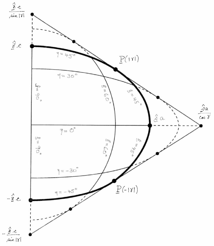
Figure 1: Bryan’s ellipsoidal coordinate system (103d) when $\gamma=45^{\circ}$ or $\gamma=-45^{\circ}$ and $2a=3c$. The fluid lies inside the heavy ellipse where either $\eta=-|\gamma|$, or $\xi=|\gamma|$, or $\eta=|\gamma|$. The points ${\bf P}(\pm|\gamma|)$ are given by equation (104), $\hat{\bf s}$ and $\hat{\bf z}$ being unit vectors in the direction of increasing $s$ and $z$.

Figure 1 shows the curvilinear coordinate system $(\xi,\,\eta)$ generated by a typical $\gamma$ satisfying (100a). In that figure, the two oblique straight lines are drawn so as to be tangent to (102) at the points ${\bf P}(\pm\gamma)$, where

$${\bf P}(\gamma)\ =\ {\hat{\bf s}}\,a\,\cos\,\gamma\ +\ {\hat{\bf z}}\,c\,\sin\,\gamma\,,$$ (104)

${\hat{\bf s}}$ being the unit vector in the $s$ direction in the $(s,z)$ plane. All the level curves of $\xi$ and $\eta$ obtained from (103d) are arcs of half-ellipses tangent to those two oblique lines. The level curves $\xi$ = constant belong to half-ellipses which intersect (102) between ${\bf P}(\pm\gamma)$ and the $z$ axis, while the level curves $\eta$ = constant belong to the half-ellipses which intersect (102) between ${\bf P}(\pm\gamma)$ and $a{\hat{\bf s}}$. The level curve $\xi\ =\ \pi/2$ is the segment of the $z$-axis connecting $-c{\hat{\bf z}}$ and $c{\hat{\bf z}}$. The level curve $\xi\ =\ |\gamma|$ is the part of (102) connecting ${\bf P}(\gamma)$ and ${\bf P}(-\gamma)$. The level curve $\eta\ =\ -|\gamma|$ is the part of (102) connecting $-c\,{\hat{\bf z}}$ and ${\bf P}(-|\gamma|)$. The level curve $\eta\ =\ |\gamma|$ is the part of (102) connecting $c\,{\hat{\bf z}}$ and ${\bf P}(|\gamma|)$. The level curve $\eta\ =\ 0$ is the segment of the $s$ axis connecting the origin and $a{\bf\hat{s}}$.

In terms of the coordinates $(\xi,\eta)$ the partial derivatives $\partial_{s}$ and $\partial_{z}$ are as follows:

$$aD(\xi,\eta)\sec\gamma\partial_{s}=\sin\xi\cos\eta\partial_{\xi}-\cos\xi\sin\eta\partial_{\eta}$$ (105a)

$$cD(\xi,\eta)\csc\gamma\partial_{z}=\cos\xi\sin\eta\partial_{\xi}-\sin\xi\cos\eta\partial_{\eta}$$ (105b)

where

$$D(\xi,\eta)\ =\ \cos^{2}\xi-\cos^{2}\eta\,.$$ (105c)

Straightforward calculation using (100b) then shows that

$$(a\sec\gamma)^{2}\,D(\xi,\eta)\,[\partial_{s}^{2}\ +\ s^{-1}\,\partial_{s}\ -$$

$$m^{2}s-(\lambda^{-2}-1)\partial_{z}^{2}]\ =\ L_{\eta}^{(m)}\ -\ L_{\xi}^{(m)}$$ (106a)

where

$$L_{\eta}^{(m)}\ =\ \partial_{\eta}^{2}\ -\ \tan\eta\,\partial_{\eta}\ -\ m^{2}(\sec\eta)^{2}\,.$$ (106b)

In the same way,

$$\begin{array}[]{l}D(\xi,\eta)\sin^{2}\gamma\left[s\partial_{s}+m\lambda^{-1}-(a/c)^{2}(\lambda^{-2}-1)z\partial_{z}\right]\\ \\ =D(\eta,\gamma)\sin\xi\cos\xi\partial_{\xi}+D(\gamma,\xi)\sin\eta\cos\eta\partial_{\eta}\\ \\ -D(\eta,\xi)m\lambda^{-1}\sin^{2}\gamma.\end{array}$$ (107)

Thus the Poincaré equation (98b) becomes

$$L_{\eta}^{(m)}\,\tilde{q}\ =\ L_{\xi}^{(m)}\,\tilde{q}$$ (108)

and the boundary condition (98a) separates into three parts corresponding to the three arcs into which ${\bf P}(\gamma)$ and ${\bf P}(-\gamma)$ divide the half-ellipse (102). To satisfy (98a) $\tilde{q}$ must behave as follows: for $|\gamma|<\xi<\pi/2$ one must have

$$\begin{array}[]{l}[\sin\eta\cos\eta\partial_{\eta}-mh(\gamma)\sin\gamma]\tilde{q}(\xi,\eta)=0\\ \\ {\rm at}\ \ \ \eta\ =\ \pm\gamma\,;\end{array}$$ (109a)

and for $$-|\gamma|<\eta<|\gamma|$$ one must have

$$\begin{array}[]{l}[\sin\xi\cos\xi\partial_{\xi}-mh(\gamma)\sin\gamma]\tilde{q}(\xi,\eta)=0\\ \\ {\rm at}\ \ \ \xi\ =\ |\gamma|\,.\end{array}$$ (109b)

Because of (108), a particular solution of (98b) can be obtained by choosing any integer $l\,\geq\,|\,m|$ and setting

$$\tilde{q}(\xi,\eta)\ =\ P_{l}^{m}(\sin\,\xi)\,P_{l}^{m}(\sin\,\eta)$$ (110a)

where $$P_{l}^{m}$$ is the associated Legendre function,

$$P_{l}^{m}(\mu)\ =\ (2^{l}\,l!)^{-1}\,(1-\mu^{2})^{m/2}\,\partial_{\mu}^{l+m}\,(\mu^{2}\ -\ 1)^{l}\,.$$ (110b)

This $\tilde{q}$ will also satisfy the boundary conditions (98a) if it satisfies (109b), that is, if

$$\begin{array}[]{l}[\sin\eta\cos\eta\partial_{\eta}-mh(\gamma)\sin\gamma]P_{l}^{m}(\sin\eta)=0\\ \\ {\rm at}\ \ \ \eta\ =\ \pm\gamma\end{array}$$ (111a)

and also

$$\begin{array}[]{l}[\sin\xi\cos\xi\partial_{\xi}-mh(\gamma)\sin\gamma]P_{l}^{m}(\sin\xi)=0\\ \\ {\rm at}\ \ \ \xi\ =\ |\gamma|\,.\end{array}$$ (111b)

Obviously (111a) implies (111b). Moreover, the left side of (111a) has the same parity in $\eta$ as does $P_{l}^{m}(\sin\,\eta)$, so if (111a) is satisfied for $\eta\ =\ \gamma$ it is also satisfied for $\eta\ =\ -\gamma$. At $\eta\ =\ \gamma$, (111a) reduces to

$$[\,\cos\,\eta\,\partial_{\eta}\ -\ mh(\eta)\,]\ P_{l}^{m}(\sin\,\eta)\ =\ 0$$ (112a)

where, because of (100a),

$$0<|\eta|<\pi/2\,.$$ (112b)

Note that when $m\ =\ 0$ the choice $l\ =\ 0$ is of no interest because then in (110a) $\tilde{q}\ =\ 1$ so (8) gives ${\bf v}={\bf 0}$.

Now we can summarize Bryan’s (1889) recipe for constructing some eigenfunctions $q$ and their corresponding eigenvalues $\lambda$ in the Poincaré pressure problem (9b): choose any integer $l\ \geq\ 1$ and any integer $m$ satisfying $-l\ \leq\ m\ \leq\ l$. Find a root $\eta$ of (112b) and set $\gamma=\eta$. Then use this $\gamma$ to generate a curvilinear coordinate system (103d) inside the fluid ellipsoid. Choose

$$q(s,\,\phi\,,\,z)\ =\ e^{{im}\phi}\,P_{l}^{m}(\sin\,\xi)\,P_{l}^{m}(\sin\,\eta)$$ (113)

where $s$ and $z$ are given by (103d). Finally, calculate $\lambda$ from $\gamma$ via (101b).