No Downlink Pilots are Needed in TDD Massive MIMO

Abstract

We consider the Massive Multiple-Input Multiple-Output downlink with maximum-ratio and zero-forcing processing and time-division duplex operation. To decode, the users must know their instantaneous effective channel gain. Conventionally, it is assumed that by virtue of channel hardening, this instantaneous gain is close to its average and hence that users can rely on knowledge of that average (also known as statistical channel information). However, in some propagation environments, such as keyhole channels, channel hardening does not hold.

We propose a blind algorithm to estimate the effective channel gain at each user, that does not require any downlink pilots. We derive a capacity lower bound of each user for our proposed scheme, applicable to any propagation channel. Compared to the case of no downlink pilots (relying on channel hardening), and compared to training-based estimation using downlink pilots, our blind algorithm performs significantly better. The difference is especially pronounced in environments that do not offer channel hardening.

I Introduction

In Massive Multiple-Input Multiple-Output (MIMO), the base station (BS) is equipped with a large antenna array (with hundreds of antennas) that simultaneously serves many (tens or more of) users. It is a key, scalable technology for next generations of wireless networks, due to its promised huge energy efficiency and spectral efficiency [2, 3, 4, 5, 6, 7]. In Massive MIMO, time-division duplex (TDD) operation is preferable, because the amount of pilot resources required does not depend on the number of BS antennas. With TDD, the BS obtains the channel state information (CSI) through uplink training. This CSI is used to detect the signals transmitted from users in the uplink. On downlink, owing to the reciprocity of propagation, CSI acquired at the BS is used for precoding. Each user receives an effective (scalar) channel gain multiplied by the desired symbol, plus interference and noise. To coherently detect the desired symbol, each user should know its effective channel gain.

Conventionally, each user is assumed to approximate its instantaneous channel gain by its mean [8, 9, 10]. This is known to work well in Rayleigh fading. Since Rayleigh fading channels harden when the number of BS antennas is large (the effective channel gains become nearly deterministic), the effective channel gain is close to its mean. Thus, using the mean of this gain for signal detection works very well. This way, downlink pilots are avoided and users only need to know the channel statistics. However, for small or moderate numbers of antennas, the gain may still deviate significantly from its mean. Also, in propagation environments where the channel does not harden, using the mean of the effective gain as substitute for its true value may result in poor performance even with large numbers of antennas.

The users may estimate their effective channel gain by using downlink pilots, see [2] for single-cell systems and [11] for multi-cell systems. Effectively, these downlink pilots are orthogonal between the users and beamformed along with the downlink data. The users may use, for example, linear minimum mean-square error (MMSE) techniques for the estimation of this gain. The downlink rates of multi-cell systems for maximum-ratio (MR) and zero-forcing (ZF) precoders with and without downlink pilots were analyzed in [12]. The effect of using outdated gain estimates at the users was investigated in [13]. Compared with the case when the users rely on statistical channel knowledge, the downlink-pilot based schemes improve the system performance in low-mobility environments (where the coherence interval is long). However, in high-mobility environments, they do not work well, owing to the large requirement of downlink training resources; this required overhead is proportional to the number of multiplexed users. A better way of estimating the effective channel gain, which requires less resources than the transmission of downlink pilots does, would be desirable.

Inspired by the above discussion, in this paper, we consider the Massive MIMO downlink with TDD operation. The BS acquires channel state information through the reception of uplink pilot signals transmitted by the users – in the conventional manner, and when transmitting data to the users, it applies MR or ZF processing with slow time-scale power control. For this system, we propose a simple blind method for the estimation of the effective gain, that each user should independently perform, and which does not require any downlink pilots. Our proposed method exploits the asymptotic properties of the received data in each coherence interval. Our specific contributions are:

• We give a formal definition of channel hardening, and an associated criterion that can be used to test if channel hardening holds. Then we examine two important propagation scenarios: independent Rayleigh fading, and keyhole channels. We show that Rayleigh fading channels harden, but keyhole channels do not.

• We propose a blind channel estimation scheme, that each user applies in the downlink. This scheme exploits the asymptotic properties of the sample average power of the received signal per coherence interval. We presented a preliminary version of this algorithm in [1].

• We derive a rigorous capacity lower bound for Massive MIMO with estimated downlink channel gains. This bound can be applied to any types of channels and can be used to analyze the performance of any downlink channel estimation method.

• Via numerical results we show that, in hardening propagation environments, the performance of our proposed blind scheme is comparable to the use of only statistical channel information (approximating the gain by its mean). In contrast, in non-hardening propagation environments, our proposed scheme performs much better than the use of statistical channel information only. The results also show that our blind method uniformly outperforms schemes based on downlink pilots [2, 11].

Notation: We use boldface upper- and lower-case letters to denote matrices and column vectors, respectively. Specific notation and symbols used in this paper are listed as follows:

$()^{\ast}$, $()^{T}$, and $()^{H}$	Conjugate, transpose, and transpose
	conjugate
$\det\left(\cdot\right)$ and $\mathrm{Tr}\left(\cdot\right)$	Determinant and trace of a matrix
$\mathcal{CN}\left({\mathbf{0}},{\mathbf{\Sigma}}\right)$	Circularly symmetric complex
	Gaussian vector with zero mean
	and covariance matrix $\mathbf{\Sigma}$
$|\cdot|$, $\|\cdot\|$	Absolute value, Euclidean norm
$\mathsf{E}\left\{\cdot\right\}$, $\operatorname{\mathsf{Var}}\left\{{\cdot}\right\}$	Expectation, variance operators
$\mathop{\to}\limits^{P}$	Convergence in probability
${\mathbf{I}}_{n}$	$n\times n$ identity matrix
$\left[{\mathbf{A}}\right]_{k}$, ${\mathbf{a}}_{k}$	The $k$th column of ${\mathbf{A}}$.

II System Model

We consider a single-cell Massive MIMO system with an $M$-antenna BS and $K$ single-antenna users, where $M>K$. The channel between the BS and the $k$th user is an $M\times 1$ channel vector, denoted by ${\mathbf{g}}_{k}$, and is modelled as:

$${\mathbf{g}}_{k}=\sqrt{\beta_{k}}{\mathbf{h}}_{k},$$ (1)

where $\beta_{k}$ represents large-scale fading which is constant over many coherence intervals, and ${\mathbf{h}}_{k}$ is an $M\times 1$ small-scale fading channel vector. We assume that the elements of ${\mathbf{h}}_{k}$ are uncorrelated, zero-mean and unit-variance random variables (RVs) which are not necessarily Gaussian distributed. Furthermore, ${\mathbf{h}}_{k}$ and ${\mathbf{h}}_{k^{\prime}}$ are assumed to be independent, for $k\neq k^{\prime}$. The $m$th elements of ${\mathbf{g}}_{k}$ and ${\mathbf{h}}_{k}$ are denoted by $g_{k}^{m}$ and $h_{k}^{m}$, respectively.

Here, we focus on the downlink data transmission with TDD operation. The BS uses the channel estimates obtained in the uplink training phase, and applies MR or ZF processing to transmit data to all users in the same time-frequency resource.

II-A Uplink Training

Let $\tau_{\mathrm{c}}$ be the length of the coherence interval (in symbols). For each coherence interval, let $\tau_{\mathrm{u,p}}$ be the length of uplink training duration (in symbols). All users simultaneously send pilot sequences of length $\tau_{\mathrm{u,p}}$ symbols each to the BS. We assume that these pilot sequences are pairwisely orthogonal. So it is required that $\tau_{\mathrm{u,p}}\geq K$. The linear MMSE estimate of ${\mathbf{g}}_{k}$ is given by [14]

$$\hat{{\mathbf{g}}}_{k}=\frac{\tau_{\mathrm{u,p}}\rho_{\mathrm{u}}\beta_{k}}{\tau_{\mathrm{u,p}}\rho_{\mathrm{u}}\beta_{k}+1}{\mathbf{g}}_{k}+\frac{\sqrt{\tau_{\mathrm{u,p}}\rho_{\mathrm{u}}}\beta_{k}}{\tau_{\mathrm{u,p}}\rho_{\mathrm{u}}\beta_{k}+1}{\mathbf{w}}_{\text{p},k},$$ (2)

where ${\mathbf{w}}_{\text{p},k}\sim\mathcal{CN}\left({0},{{\mathbf{I}}_{M}}\right)$ independent of ${\mathbf{g}}_{k}$, and $\rho_{\mathrm{u}}$ is the transmit signal-to-noise ratio (SNR) of each pilot symbol.

The variance of the $m$th element of $\hat{{\mathbf{g}}}_{k}$ is given by

$$\operatorname{\mathsf{Var}}\left\{{\hat{g}_{k}^{m}}\right\}=\mathsf{E}\left\{{|\hat{g}_{k}^{m}|^{2}}\right\}=\frac{\tau_{\mathrm{u,p}}\rho_{\mathrm{u}}\beta_{k}^{2}}{\tau_{\mathrm{u,p}}\rho_{\mathrm{u}}\beta_{k}+1}\triangleq\gamma_{k}.$$ (3)

Let $\tilde{{\mathbf{g}}}_{k}={\mathbf{g}}_{k}-\hat{{\mathbf{g}}}_{k}$ be the channel estimation error, and $\tilde{g}_{k}^{m}$ be the $m$th element of $\tilde{{\mathbf{g}}}_{k}$. Then from the properties of linear MMSE estimation, $\tilde{g}_{k}^{m}$ and $\hat{g}_{k}^{m}$ are uncorrelated, and

$$\operatorname{\mathsf{Var}}\left\{{\tilde{g}_{k}^{m}}\right\}=\mathsf{E}\left\{{|\tilde{g}_{k}^{m}|^{2}}\right\}=\beta_{k}-\gamma_{k}.$$ (4)

In the special case where ${\mathbf{g}}_{k}$ is Gaussian distributed (corresponding to Rayleigh fading channels), the linear MMSE estimator becomes the MMSE estimator and $\tilde{g}_{k}^{m}$ is independent of $\hat{g}_{k}^{m}$.

II-B Downlink Data Transmission

Let $s_{k}(n)$ be the $n$th symbol intended for the $k$th user. We assume that $\mathsf{E}\left\{{{\mathbf{s}}(n){\mathbf{s}}(n)^{H}}\right\}={\mathbf{I}}_{K}$, where ${\mathbf{s}}(n)\triangleq[s_{1}(n),\ldots,s_{K}(n)]^{T}$. With linear processing, the $M\times 1$ precoded signal vector is

$${\mathbf{x}}(n)=\sqrt{\rho_{\mathrm{d}}}\sum_{k=1}^{K}\sqrt{\eta_{k}}{\mathbf{a}}_{k}s_{k}(n),$$ (5)

where $\{{\mathbf{a}}_{k}\}$, $k=1,\ldots,K$, are the precoding vectors which are functions of the channel estimate $\hat{{\mathbf{G}}}\triangleq[\hat{{\mathbf{g}}}_{1},\ldots,\hat{{\mathbf{g}}}_{K}]$, ${\rho_{\mathrm{d}}}$ is the (normalized) average transmit power, $\{\eta_{k}\}$ are the power coefficients, and ${\mathbf{D}}_{\eta}$ is a diagonal matrix with $\{\eta_{k}\}$ on its diagonal. For a given $\{{\mathbf{a}}_{k}\}$, the power control coefficients $\{\eta_{k}\}$ are chosen to satisfy an average power constraint at the BS:

$$\mathsf{E}\left\{{\|{\mathbf{x}}(n)\|^{2}}\right\}\leq\rho_{\mathrm{d}}.$$ (6)

The signal received at the $k$th user is

$$y_{k}(n)={\mathbf{g}}_{k}^{H}{\mathbf{x}}(n)+w_{k}(n)$$

$$=\sqrt{\rho_{\mathrm{d}}\eta_{k}}\alpha_{kk}s_{k}(n)+\sum_{k^{\prime}\neq k}^{K}\sqrt{\rho_{\mathrm{d}}\eta_{k^{\prime}}}\alpha_{kk^{\prime}}s_{k^{\prime}}(n)+w_{k}(n),$$ (7)

where $w_{k}(n)\sim\mathcal{CN}\left({0},{1}\right)$ is additive Gaussian noise, and

$$\alpha_{kk^{\prime}}\triangleq{\mathbf{g}}_{k}^{H}{\mathbf{a}}_{k^{\prime}}.$$

Then, the desired signal $s_{k}$ is decoded.

We consider two linear precoders: MR and ZF processing.

• MR processing: here the precoding vectors $\{{\mathbf{a}}_{k}\}$ are

  $${\mathbf{a}}_{k}=\frac{\hat{{\mathbf{g}}}_{k}}{\|\hat{{\mathbf{g}}}_{k}\|},\quad k=1,\ldots,K.$$ (8)

• ZF processing: here the precoding vectors are

  $${\mathbf{a}}_{k}=\frac{1}{\left\|\left[\hat{{\mathbf{G}}}\left(\hat{{\mathbf{G}}}^{H}\hat{{\mathbf{G}}}\right)^{-1}\right]_{k}\right\|}\left[\hat{{\mathbf{G}}}\left(\hat{{\mathbf{G}}}^{H}\hat{{\mathbf{G}}}\right)^{-1}\right]_{k},$$ (9)

  for $k=1,\ldots,K$.

With the precoding vectors given in (8) and (9), the power constraint (6) becomes

$$\sum_{k=1}^{K}\eta_{k}\leq 1.$$ (10)

III Preliminaries of Channel Hardening

One motivation of this work is that Massive MIMO channels may not always harden. In this section we discuss the channel hardening phenomena. We specifically study channel hardening for independent Rayleigh fading and for keyhole channels.

Channel hardening is a phenomenon where the norms of the channel vectors $\{{\mathbf{g}}_{k}\}$, $k=1,\ldots,K$, fluctuate only little. We say that the propagation offers channel hardening if

$$\frac{\|{\mathbf{g}}_{k}\|^{2}}{\mathsf{E}\left\{{\|{\mathbf{g}}_{k}\|^{2}}\right\}}~{}\mathop{\to}\limits^{P}~{}1,\quad\text{as}~{}M\to\infty,\quad k=1,\ldots,K.$$ (11)

III-A Advantages of Channel Hardening

If the BS and the users know the channel ${\mathbf{G}}$ perfectly, the channel is deterministic and its sum-capacity is given by [15]

$$C=\max_{\eta_{k}\geq 0,\sum_{k=1}^{K}\eta_{k}\leq 1}\log_{2}\det\left({\mathbf{I}}_{M}+\rho_{\mathrm{d}}{\mathbf{G}}{\mathbf{D}}_{\eta}{\mathbf{G}}^{H}\right),$$ (12)

where ${\mathbf{D}}_{\eta}$ is the diagonal matrix whose $k$th diagonal element is the power control coefficient $\eta_{k}$.

In Massive MIMO, for most propagation environments, we have asymptotically favorable propagation [16], i.e. $\frac{{\mathbf{g}}_{k}^{H}{\mathbf{g}}_{k^{\prime}}}{M}\to 0$, as $M\to\infty$, for $k\neq k^{\prime}$. In addition, if the channel hardens, i.e., $\frac{\|{\mathbf{g}}_{k}\|^{2}}{M}\to\mathsf{E}\left\{{{\left\|{\mathbf{g}}_{k}\right\|^{2}}}\right\}=\beta_{k}$, as $M\to\infty$, then we have, for fixed $K$,

$$C-\max_{\eta_{k}\geq 0,\sum_{k=1}^{K}\eta_{k}\leq 1}\sum_{k=1}^{K}\log_{2}\left(1+\rho_{\mathrm{d}}\eta_{k}\beta_{k}M\right)$$

$$=C-\!\!\!\max_{\eta_{k}\geq 0,\sum_{k=1}^{K}\eta_{k}\leq 1}\!\!\!\!\!\!\log_{2}\det\!\!\left({\mathbf{I}}_{K}\!+\!\rho_{\mathrm{d}}{\mathbf{D}}_{\eta}M\left[\begin{array}[]{ccc}\beta_{1}&\cdots&0\\ \vdots&\ddots&\vdots\\ 0&\cdots&\beta_{K}\\ \end{array}\right]\right)$$ (16)

$$=\!\!\!\!\!\!\max_{\eta_{k}\geq 0,\sum_{k=1}^{K}\eta_{k}\leq 1}\!\!\!\!\!\!\log_{2}\det\!\!\left(\left[\begin{array}[]{ccc}\frac{1+\rho_{\mathrm{d}}\eta_{1}\|{\mathbf{g}}_{1}\|^{2}}{1+\rho_{\mathrm{d}}\eta_{1}\beta_{1}M}&\cdots&\frac{\rho_{\mathrm{d}}\eta_{1}{\mathbf{g}}_{1}^{H}{\mathbf{g}}_{K}}{1+\rho_{\mathrm{d}}\eta_{K}\beta_{K}M}\\ \vdots&\ddots&\vdots\\ \frac{\rho_{\mathrm{d}}\eta_{K}{\mathbf{g}}_{K}^{H}{\mathbf{g}}_{1}}{1+\rho_{\mathrm{d}}\eta_{1}\beta_{1}M}&\cdots&\frac{1+\rho_{\mathrm{d}}\eta_{K}\|{\mathbf{g}}_{K}\|^{2}}{1+\rho_{\mathrm{d}}\eta_{K}\beta_{K}M}\\ \end{array}\right]\right)\$$ (20)

$$\to 0,\quad\text{as}~{}M\to\infty.$$ (21)

In (III-A) we have used the facts that

$$\frac{1+\rho_{\mathrm{d}}\eta_{k}\|{\mathbf{g}}_{k}\|^{2}}{1+\rho_{\mathrm{d}}\eta_{k}\beta_{k}M}=\frac{\frac{1}{M}+\rho_{\mathrm{d}}\eta_{k}\frac{\|{\mathbf{g}}_{k}\|^{2}}{M}}{\frac{1}{M}+\rho_{\mathrm{d}}\eta_{k}\beta_{k}}\to 1,~{}\text{as}~{}M\to\infty,$$

and for $k\neq k^{\prime}$,

$$\frac{\rho_{\mathrm{d}}\eta_{k}{\mathbf{g}}_{k}^{H}{\mathbf{g}}_{k^{\prime}}}{1+\rho_{\mathrm{d}}\eta_{k^{\prime}}\beta_{k^{\prime}}M}=\frac{\rho_{\mathrm{d}}\eta_{k}{\mathbf{g}}_{k}^{H}{\mathbf{g}}_{k^{\prime}}/M}{1/M+\rho_{\mathrm{d}}\eta_{k^{\prime}}\beta_{k^{\prime}}}\to 0,\quad\text{as}~{}M\to\infty.$$

The limit in (III-A) implies that if the channel hardens, the sum-capacity (12) can be approximated for $M\gg K$ as:

$$C\approx\max_{\eta_{k}\geq 0,\sum_{k=1}^{K}\eta_{k}\leq 1}\sum_{k=1}^{K}\log_{2}\left(1+\rho_{\mathrm{d}}\eta_{k}\beta_{k}M\right),$$ (22)

which does not depend on the small-scale fading. As a consequence, the system scheduling, power allocation, and interference management can be done over the large-scale fading time scale instead of the small-scale fading time scale. Therefore, the overhead for these system designs is significantly reduced.

Another important advantage is: if the channel hardens, then we do not need instantaneous CSI at the receiver to detect the transmitted signals. What the receiver needs is only the statistical knowledge of the channel gains. This reduces the resources (power and training duration) required for channel estimation. More precisely, consider the signal received at the $k$th user given in (II-B). The $k$th user wants to detect $s_{k}$ from $y_{k}$. For this purpose, it needs to know the effective channel gain $\alpha_{kk}$. If the channel hardens, then $\alpha_{kk}\approx\mathsf{E}\left\{{\alpha_{kk}}\right\}$. Therefore, we can use the statistical properties of the channel, i.e., $\mathsf{E}\left\{{\alpha_{kk}}\right\}$ is a good estimate of $\alpha_{kk}$ when detecting $s_{k}$. This assumption is widely made in the Massive MIMO literature [8, 9, 10] and circumvents the need for downlink channel estimation.

III-B Measure of Channel Hardening

We next state a simple criterion, based on the Chebyshev inequality, to check whether the channel hardens or not. A similar method was discussed in [17]. From Chebyshev’s inequality, we have

$$\operatorname{\mathsf{Pr}}\left\{{\left|\frac{{\left\|{\mathbf{g}}_{k}\right\|^{2}}}{\mathsf{E}\left\{{{\left\|{\mathbf{g}}_{k}\right\|^{2}}}\right\}}-1\right|^{2}\leq\epsilon}\right\}$$

$$=1-\operatorname{\mathsf{Pr}}\left\{{\left|\frac{{\left\|{\mathbf{g}}_{k}\right\|^{2}}}{\mathsf{E}\left\{{{\left\|{\mathbf{g}}_{k}\right\|^{2}}}\right\}}-1\right|^{2}\geq\epsilon}\right\}$$

$$\geq 1-\frac{1}{\epsilon}\cdot\frac{\operatorname{\mathsf{Var}}\left\{{{\left\|{\mathbf{g}}_{k}\right\|^{2}}}\right\}}{\left(\mathsf{E}\left\{{{\left\|{\mathbf{g}}_{k}\right\|^{2}}}\right\}\right)^{2}},\quad\text{for any $\epsilon\geq 0$}.$$ (23)

Clearly, if

$$\frac{\operatorname{\mathsf{Var}}\left\{{{\left\|{\mathbf{g}}_{k}\right\|^{2}}}\right\}}{\left(\mathsf{E}\left\{{{\left\|{\mathbf{g}}_{k}\right\|^{2}}}\right\}\right)^{2}}\to 0,\quad\text{as}~{}M\to\infty,$$ (24)

we have channel hardening. In contrast, (11) implies

$$\frac{\operatorname{\mathsf{Var}}\left\{{{\left\|{\mathbf{g}}_{k}\right\|^{2}}}\right\}}{\left(\mathsf{E}\left\{{{\left\|{\mathbf{g}}_{k}\right\|^{2}}}\right\}\right)^{2}}\to 0,\quad\text{as}~{}M\to\infty,$$

so if (24) does not hold, then the channel does not harden. Therefore, we can use $\frac{\operatorname{\mathsf{Var}}\left\{{{\left\|{\mathbf{g}}_{k}\right\|^{2}}}\right\}}{\left(\mathsf{E}\left\{{{\left\|{\mathbf{g}}_{k}\right\|^{2}}}\right\}\right)^{2}}$ to determine if channel hardening holds for a particular propagation environment.

III-C Independent Rayleigh Fading and Keyhole Channels

In this section, we study the channel hardening property of two particular channel models: Rayleigh fading and keyhole channels.

III-C1 Independent Rayleigh Fading Channels

Consider the channel model (1) where $\{h_{k}^{m}\}$ (the elements of ${\mathbf{h}}_{k}$) are i.i.d. $\mathcal{CN}\left({0},{1}\right)$ RVs. Independent Rayleigh fading channels occur in a dense, isotropic scattering environment [18]. By using the identity $\mathsf{E}\left\{{\|{\mathbf{g}}_{k}\|^{4}}\right\}=\beta_{k}^{2}(M+1)M$ [19], we obtain

$$\frac{\operatorname{\mathsf{Var}}\left\{{{\left\|{\mathbf{g}}_{k}\right\|^{2}}}\right\}}{\left(\mathsf{E}\left\{{{\left\|{\mathbf{g}}_{k}\right\|^{2}}}\right\}\right)^{2}} =\frac{1}{\beta_{k}^{2}M^{2}}\mathsf{E}\left\{{\|{\mathbf{g}}_{k}\|^{4}}\right\}-1$$

$$=\frac{1}{M}\to 0,\quad M\to\infty.$$ (25)

Therefore, we have channel hardening.

III-C2 Keyhole Channels

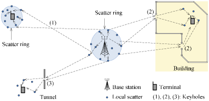
Figure 1: Examples of keyhole channels: (1)—keyhole effects occur when the distance between transmitter and receiver is large. The transmitter and the receiver have their own local scatters which yield locally uncorrelated fading. However, the scatter rings are much smaller than the distance between them, the channel becomes low rank, and hence keyhole effects occur [20]; (2)—the receiver is located inside a building, the only way for the radio wave to propagation from the transmitter to the receiver is to go through several narrow holes which can be considered as keyholes; and (3)—the transmitter and the receiver are separated by a tunnel.

A keyhole channel (or double scattering channel) appears in scenarios with rich scattering around the transmitter and receiver, and where there is a low-rank connection between the two scattering environments. The keyhole effect can occur when the radio wave goes through tunnels, corridors, or when the distance between the transmitter and receiver is large. Figure 1 shows some examples where the keyhole effect occurs in practice. This channel model has been validated both in theory and by practical experiments [21, 22, 23, 24]. Under keyhole effects, the channel vector ${\mathbf{g}}_{k}$ in (1) is modelled as [22]:

$${\mathbf{g}}_{k}=\sqrt{\beta_{k}}\sum_{j=1}^{n_{k}}c_{j}^{(k)}a_{j}^{(k)}{\mathbf{b}}_{j}^{(k)},$$ (26)

where $n_{k}$ is the number of effective keyholes, $a_{j}^{(k)}$ is the random channel gain from the $k$th user to the $j$th keyhole, ${\mathbf{b}}_{j}^{(k)}\in\mathbb{C}^{M\times 1}$ is the random channel vector between the $j$th keyhole associated with the $k$th user and the BS, and $c_{j}^{(k)}$ represents the deterministic complex gain of the $j$th keyhole associated with the $k$th user. The elements of ${\mathbf{b}}_{j}^{(k)}$ and $a_{j}^{(k)}$ are i.i.d. $\mathcal{CN}\left({0},{1}\right)$ RVs. Furthermore, the gains $\{c_{j}^{(k)}\}$ are normalized such that $\mathsf{E}\left\{{|{g}_{k}^{m}|^{2}}\right\}=\beta_{k}$. Therefore,

$$\sum_{i=1}^{n_{k}}\left|c_{i}^{(k)}\right|^{2}=1.$$ (27)

When $n_{k}=1$, we have a degenerate keyhole (single-keyhole) channel. Conversely, when $n_{k}\to\infty$, under the additional assumptions that $c_{i}^{(k)}\neq 0$ for finite $n_{k}$ and $c_{i}^{(k)}\to 0$ as $n_{k}\to\infty$, we obtain an i.i.d. Rayleigh fading channel.

We assume that different users have different sets of keyholes. This assumption is reasonable if the users are located at random in a large area, as illustrated in Figure 1. Then from the derivations in Appendix -A, we obtain

$$\frac{\operatorname{\mathsf{Var}}\left\{{{\left\|{\mathbf{g}}_{k}\right\|^{2}}}\right\}}{\left(\mathsf{E}\left\{{{\left\|{\mathbf{g}}_{k}\right\|^{2}}}\right\}\right)^{2}} =\left(1+\frac{1}{M}\right)\sum_{i=1}^{n_{k}}\left|c_{i}^{(k)}\right|^{4}+\frac{1}{M}$$

$$\to\sum_{i=1}^{n_{k}}\left|c_{i}^{(k)}\right|^{4}\neq 0,\quad M\to\infty.$$ (28)

Consequently, the keyhole channels do not harden. In addition, since $\left|c_{i}^{(k)}\right|^{2}\leq 1$, we have

$$\frac{\operatorname{\mathsf{Var}}\left\{{{\left\|{\mathbf{g}}_{k}\right\|^{2}}}\right\}}{\left(\mathsf{E}\left\{{{\left\|{\mathbf{g}}_{k}\right\|^{2}}}\right\}\right)^{2}} \leq\left(1+\frac{1}{M}\right)\sum_{i=1}^{n_{k}}\left|c_{i}^{(k)}\right|^{2}+\frac{1}{M}.$$ (29)

Using (27), (29) becomes

$$\frac{\operatorname{\mathsf{Var}}\left\{{{\left\|{\mathbf{g}}_{k}\right\|^{2}}}\right\}}{\left(\mathsf{E}\left\{{{\left\|{\mathbf{g}}_{k}\right\|^{2}}}\right\}\right)^{2}} \leq 1+\frac{2}{M},$$ (30)

where the right hand side corresponds to the case of single-keyhole channels ($n_{k}=1$). This implies that a single-keyhole channel represents the worst case in the sense that then the channel gain fluctuates the most.

IV Proposed Downlink Blind Channel Estimation Technique

The $k$th user should know the effective channel gain $\alpha_{kk}$ to coherently detect the transmitted signal $s_{k}$ from $y_{k}$ in (II-B). Most previous works on Massive MIMO assume that $\mathsf{E}\left\{{\alpha_{kk}}\right\}$ is used in lieu of the true $\alpha_{kk}$ when detecting $s_{k}$. The reason behind this is that if the channel is subject to independent Rayleigh fading (the scenario considered in most previous Massive MIMO works), it hardens when the number of BS antennas is large, and hence $\alpha_{kk}\approx\mathsf{E}\left\{{\alpha_{kk}}\right\}$; $\mathsf{E}\left\{{\alpha_{kk}}\right\}$ is then a good estimate of $\alpha_{kk}$. However, as seen in Section III, under other propagation models the channel may not always harden when $M\to\infty$ and then, using $\mathsf{E}\left\{{\alpha_{kk}}\right\}$ as the true effective channel $\alpha_{kk}$ to detect $s_{k}$ may result in poor performance.

For the reasons explained, it is desirable that the users estimate their effective channels. One way to do this is to have the BS transmit beamformed downlink pilots [2]. Then at least $K$ downlink pilot symbols are required. This can significantly reduce the spectral efficiency. For example, suppose $M=200$ antennas serve $K=50$ users, in a coherence interval of length $200$ symbols. If half of the coherence interval is used for the downlink, then with the downlink beamforming training of [2], we need to spend at least $50$ symbols for sending pilots. As a result, less than $50$ of the $100$ downlink symbols are used for payload in each coherence interval, and the insertion of the downlink pilots reduces the overall (uplink + downlink) spectral efficiency by a factor of $1/4$.

In what follows, we propose a blind channel estimation method which does not require any downlink pilots.

IV-A Downlink Blind Channel Estimation Algorithm

We next describe our downlink blind channel estimation algorithm, a refined version of the scheme in [1]. Consider the sample average power of the received signal at the $k$th user per coherence interval:

$$\xi_{k}\triangleq\frac{|y_{k}(1)|^{2}+|y_{k}(2)|^{2}+\ldots+|y_{k}(\tau_{\mathrm{d}})|^{2}}{\tau_{\mathrm{d}}},$$ (31)

where $y_{k}(n)$ is the $n$th sample received at the $k$th user and $\tau_{\mathrm{d}}$ is the number of symbols per coherence interval spent on downlink transmission. From (II-B), and by using the law of large numbers, we have, as $\tau_{\mathrm{d}}\to\infty$,

$$\xi_{k}-\left(\rho_{\mathrm{d}}\eta_{k}\left|\alpha_{kk}\right|^{2}+\sum_{k^{\prime}\neq k}^{K}\rho_{\mathrm{d}}\eta_{k^{\prime}}\left|\alpha_{kk^{\prime}}\right|^{2}+1\right)~{}\mathop{\to}\limits^{P}~{}0.$$ (32)

Since $\sum_{k^{\prime}\neq k}^{K}\rho_{\mathrm{d}}\eta_{k^{\prime}}\left|\alpha_{kk^{\prime}}\right|^{2}$ is a sum of many terms, it can be approximated by its mean (this follows from the law of large numbers). As a consequence, when $K$, and $\tau_{\mathrm{d}}$ are large, $\xi_{k}$ in (31) can be approximated as follows:

$$\xi_{k}\approx\rho_{\mathrm{d}}\eta_{k}|\alpha_{kk}|^{2}+\rho_{\mathrm{d}}\mathsf{E}\left\{{\sum_{k^{\prime}\neq k}^{K}\eta_{k^{\prime}}|\alpha_{kk^{\prime}}|^{2}}\right\}+1.$$ (33)

Furthermore, the approximation (33) is still good even if $K$ is small. The reason is that when $K$ is small, with high probability the term $\sum_{k^{\prime}\neq k}^{K}\eta_{k^{\prime}}|\alpha_{kk^{\prime}}|^{2}$ is much smaller than $\eta_{k}|\alpha_{kk}|^{2}$, since with high probability $|\alpha_{kk^{\prime}}|^{2}\ll|\alpha_{kk}|^{2}$. As a result, $\sum_{k^{\prime}\neq k}^{K}\eta_{k^{\prime}}|\alpha_{kk^{\prime}}|^{2}$ can be approximated by its mean even for small $K$. (In fact, in the special case of $K=1$, this sum is zero.)

Equation (33) enables us to estimate the amplitude of the effective channel gain $\alpha_{kk}$ using the received samples via $\xi_{k}$ as follows:

$$\widehat{|\alpha_{kk}|}=\sqrt{\frac{\xi_{k}-1-\rho_{\mathrm{d}}\mathsf{E}\left\{{\sum_{k^{\prime}\neq k}^{K}\eta_{k^{\prime}}|\alpha_{kk^{\prime}}|^{2}}\right\}}{\rho_{\mathrm{d}}\eta_{k}}}.$$ (34)

In case the argument of the square root is non-positive, we set the estimate $|\alpha_{kk}|$ equal to $\mathsf{E}\left\{{|\alpha_{kk}|}\right\}$.

For completeness, the $k$th user also needs to estimate the phase of $\alpha_{kk}$. When $M$ is large, with high probability, the real part of $\alpha_{kk}$ is much larger than the imaginary part of $\alpha_{kk}$. Thus, the phase of $\alpha_{kk}$ is very small and can be set to zero. Based on that observation, we propose to treat the estimate of $|\alpha_{kk}|$ as the estimate of the true $\alpha_{kk}$: $\hat{\alpha}_{kk}=\widehat{|\alpha_{kk}|}$

The algorithm for estimating the downlink effective channel gain $\alpha_{kk}$ is summarized as follows:

Algorithm 1

(Blind downlink channel estimation method) 1. For each coherence interval, using a data block of $\tau_{\mathrm{d}}$ samples $y_{k}(n)$, compute $\xi_{k}$ according to (31). 2. The $k$th user acquires $\eta_{k}$ and $\mathsf{E}\left\{{\sum_{k^{\prime}\neq k}^{K}\eta_{k^{\prime}}|\alpha_{kk^{\prime}}|^{2}}\right\}$. See Remark 1 for a detailed discussion on how to acquire these values. 3. The estimate of the effective channel gain $\alpha_{kk}$ is as $\displaystyle\hat{\alpha}_{kk}\!=\!\left\{\!\begin{array}[]{l}\sqrt{\frac{\xi_{k}-1-\rho_{\mathrm{d}}\mathsf{E}\left\{{\sum_{k^{\prime}\neq k}^{K}\eta_{k^{\prime}}|\alpha_{kk^{\prime}}|^{2}}\right\}}{\rho_{\mathrm{d}}\eta_{k}}},\\ \quad\text{if $\xi_{k}>1+\rho_{\mathrm{d}}\mathsf{E}\left\{{\sum_{k^{\prime}\neq k}^{K}\eta_{k^{\prime}}|\alpha_{kk^{\prime}}|^{2}}\right\}$}\\ \mathsf{E}\left\{{|\alpha_{kk}|}\right\},\quad\text{otherwise}.\\ \end{array}\right.$ (38)

Remark 1

To implement Algorithm 1, the $k$th user has to know $\eta_{k}$ and $\mathsf{E}\left\{{\sum_{k^{\prime}\neq k}^{K}\eta_{k^{\prime}}|\alpha_{kk^{\prime}}|^{2}}\right\}$. We assume that the $k$th user knows these values. This assumption is reasonable since these values depend only on the large-scale fading coefficients, which stay constant over many coherence intervals. The BS can compute these values and inform the $k$th user about them. In addition $\mathsf{E}\left\{{\sum_{k^{\prime}\neq k}^{K}\eta_{k^{\prime}}|\alpha_{kk^{\prime}}|^{2}}\right\}$ can be expressed in closed form (except for in the case of ZF processing with keyhole channels) as follows:

$$\mathsf{E}\left\{{\sum_{k^{\prime}\neq k}^{K}\eta_{k^{\prime}}|\alpha_{kk^{\prime}}|^{2}}\right\}\!=\left\{\!\!\begin{array}[]{l}\sum\limits_{k^{\prime}\neq k}^{K}\eta_{k^{\prime}}\beta_{k},\quad\text{for MR,}\\ \text{(Rayleigh/keyhole channels)}\\ \sum\limits_{k^{\prime}\neq k}^{K}\eta_{k^{\prime}}(\beta_{k}-\gamma_{k}),~{}\text{for ZF.}\\ \text{(Rayleigh channels)}\\ \end{array}\right.$$ (43)

Detailed derivations of (43) are presented in Appendix -B.

IV-B Asymptotic Performance Analysis

In this section, we analyze the accuracy of our proposed downlink blind channel estimation scheme when $\tau_{\mathrm{c}}$ and $M$ go to infinity for two specific propagation channels: Rayleigh fading and keyhole channels. We use the model (26) for keyhole channels. When $\tau_{\mathrm{c}}\to\infty$, $\xi_{k}$ in (31) is equal to its asymptotic value:

$$\xi_{k}-\left(\rho_{\mathrm{d}}\eta_{k}\left|\alpha_{kk}\right|^{2}+\sum_{k^{\prime}\neq k}^{K}\rho_{\mathrm{d}}\eta_{k^{\prime}}\left|\alpha_{kk^{\prime}}\right|^{2}+1\right)\to 0,$$ (44)

and hence, the channel estimate $\hat{\alpha}_{kk}$ in (38) becomes

$$\hat{\alpha}_{kk}=\left\{\begin{array}[]{l}\sqrt{|\alpha_{kk}|^{2}+\sum\limits_{k^{\prime}\neq k}^{K}\frac{\eta_{k^{\prime}}}{\eta_{k}}\left(|\alpha_{kk^{\prime}}|^{2}-\mathsf{E}\left\{{|\alpha_{kk^{\prime}}|^{2}}\right\}\right)},\\ \vspace{-0.7cm}\\ \hskip 34.14322pt\text{if $\xi_{k}>1+\rho_{\mathrm{d}}\mathsf{E}\left\{{\sum\limits_{k^{\prime}\neq k}^{K}\eta_{k^{\prime}}|\alpha_{kk^{\prime}}|^{2}}\right\}$},\\ \mathsf{E}\left\{{|\alpha_{kk}|}\right\},\quad\text{otherwise}.\\ \end{array}\right.$$ (49)

Since $\tau_{\mathrm{c}}\to\infty$, it is reasonable to assume that the BS can perfectly estimate the channels in the uplink training phase, i.e., we have $\hat{{\mathbf{G}}}={\mathbf{G}}$. (This can be achieved by using very long uplink training duration.) With this assumption, $\alpha_{kk}$ is a positive real value. Thus, (49) can be rewritten as

$$\frac{\hat{\alpha}_{kk}}{\alpha_{kk}}=\left\{\begin{array}[]{l}\sqrt{1+\sum\limits_{k^{\prime}\neq k}^{K}\frac{\eta_{k^{\prime}}}{\eta_{k}}\frac{|\alpha_{kk^{\prime}}|^{2}-\mathsf{E}\left\{{|\alpha_{kk^{\prime}}|^{2}}\right\}}{\alpha_{kk}^{2}}},\\ \hskip 28.45274pt\text{if $\xi_{k}>1+\rho_{\mathrm{d}}\mathsf{E}\left\{{\sum\limits_{k^{\prime}\neq k}^{K}\eta_{k^{\prime}}|\alpha_{kk^{\prime}}|^{2}}\right\}$},\\ \frac{\mathsf{E}\left\{{\alpha_{kk}}\right\}}{\alpha_{kk}},\quad\text{otherwise}.\\ \end{array}\right.$$ (53)

IV-B1 Maximum-Ratio Processing

With MR processing, from (43) and (53), we have

$$\frac{\hat{\alpha}_{kk}}{\alpha_{kk}}=\left\{\begin{array}[]{l}\sqrt{1+\sum\limits_{k^{\prime}\neq k}^{K}\frac{\eta_{k^{\prime}}}{\eta_{k}}\frac{\left|\frac{{\mathbf{g}}_{k}^{H}{\mathbf{g}}_{k^{\prime}}}{\left\|{\mathbf{g}}_{k^{\prime}}\right\|}\right|^{2}-\beta_{k}}{\left\|{\mathbf{g}}_{k}\right\|^{2}}},\\ \hskip 54.06006pt\text{if $\xi_{k}>1+\rho_{\mathrm{d}}\sum\limits_{k^{\prime}\neq k}^{K}\eta_{k^{\prime}}\beta_{k}$},\\ \frac{\mathsf{E}\left\{{\left\|{\mathbf{g}}_{k}\right\|}\right\}}{\left\|{\mathbf{g}}_{k}\right\|},\quad\text{otherwise}.\\ \end{array}\right.$$ (57)

• Rayleigh fading channels: Under Rayleigh fading channels, $\alpha_{kk}=\left\|{\mathbf{g}}_{k}\right\|$, and hence,

  $$\operatorname{\mathsf{Pr}}\left\{{\xi_{k}>1+\rho_{\mathrm{d}}\sum_{k^{\prime}\neq k}^{K}\eta_{k^{\prime}}\beta_{k}}\right\}$$

  $$=\operatorname{\mathsf{Pr}}\left\{{1+\sum_{k^{\prime}=1}^{K}\rho_{\mathrm{d}}\eta_{k^{\prime}}\left|\alpha_{kk^{\prime}}\right|^{2}>1+\rho_{\mathrm{d}}\sum_{k^{\prime}\neq k}^{K}\eta_{k^{\prime}}\beta_{k}}\right\}$$

  $$\geq\operatorname{\mathsf{Pr}}\left\{{\rho_{\mathrm{d}}\eta_{k}\left|\alpha_{kk}\right|^{2}>\rho_{\mathrm{d}}\sum_{k^{\prime}\neq k}^{K}\eta_{k^{\prime}}\beta_{k}}\right\}$$

  $$=\operatorname{\mathsf{Pr}}\left\{{\frac{1}{M}\left\|{\mathbf{g}}_{k}\right\|^{2}>\frac{1}{M}\sum_{k^{\prime}\neq k}^{K}\frac{\eta_{k^{\prime}}}{\eta_{k}}\beta_{k}}\right\}$$

  $$\to~{}1,\quad\text{as $M\to\infty$},$$ (58)

  where the convergence follows the fact that $\frac{1}{M}\left\|{\mathbf{g}}_{k}\right\|^{2}\to\beta_{k}$ and $\frac{1}{M}\sum_{k^{\prime}\neq k}^{K}\frac{\eta_{k^{\prime}}}{\eta_{k}}\beta_{k}\to 0$, as $M\to\infty$.

  In addition, by the law of large numbers,

  $$\frac{\left|\frac{{\mathbf{g}}_{k}^{H}{\mathbf{g}}_{k^{\prime}}}{\left\|{\mathbf{g}}_{k^{\prime}}\right\|}\right|^{2}-\beta_{k}}{\left\|{\mathbf{g}}_{k}\right\|^{2}} =\left(\left|\frac{{\mathbf{g}}_{k}^{H}{\mathbf{g}}_{k^{\prime}}}{M}\right|^{2}\frac{M}{\left\|{\mathbf{g}}_{k^{\prime}}\right\|^{2}}-\frac{\beta_{k}}{M}\right)\frac{M}{\left\|{\mathbf{g}}_{k}\right\|^{2}}$$

  $$\to~{}0,\quad\text{as $M\to\infty$}.$$ (59)

  From (57), (- ‣ IV-B1), and (- ‣ IV-B1), we obtain

  $$\frac{\hat{\alpha}_{kk}}{\alpha_{kk}}\to~{}1,\quad\text{as $M\to\infty$}.$$ (60)

  Our proposed scheme is expected to work very well at large $\tau_{\mathrm{c}}$ and $M$.

• Keyhole channels: Following a similar methodology used in the case of Rayleigh fading, and using the identity

  $$\frac{{\mathbf{g}}_{k}^{H}{\mathbf{g}}_{k^{\prime}}}{\|{\mathbf{g}}_{k^{\prime}}\|}=\sqrt{\beta_{k}}\sum_{j=1}^{n_{k}}c_{j}^{(k)}a_{j}^{(k)}\nu_{j}^{(k)},$$ (61)

  where $\nu_{j}^{(k)}\triangleq\frac{\left({\mathbf{b}}_{j}^{(k^{\prime})}\right)^{H}{\mathbf{g}}_{k^{\prime}}}{\|{\mathbf{g}}_{k^{\prime}}\|}$ is $\mathcal{CN}\left({0},{1}\right)$ distributed, we can arrive at the same result as (60). The random variable $\nu_{j}^{(k)}$ is Gaussian due to the fact that conditioned on ${\mathbf{g}}_{k^{\prime}}$, $\nu_{j}^{(k)}$ is a Gaussian RV with zero mean and unit variance which is independent of ${\mathbf{g}}_{k^{\prime}}$.

IV-B2 Zero-forcing Processing

With ZF processing, when $\tau_{\mathrm{c}}\to\infty$,

$$\frac{\hat{\alpha}_{kk}}{\alpha_{kk}}\to~{}1,\quad\text{as $M\to\infty$}.$$ (62)

This follows from (44) and the fact that $\alpha_{kk^{\prime}}\to 0$, for $k\neq k^{\prime}$.

V Capacity Lower Bound

Next, we give a new capacity lower bound for Massive MIMO with downlink channel gain estimation. It can be applied, in particular, to our proposed blind channel estimation scheme. Denote by ${\mathbf{y}}_{k}\triangleq[y_{k}(1)~{}\ldots~{}y_{k}(\tau_{\mathrm{d}})]^{T}$, ${\mathbf{s}}_{k}\triangleq[s_{k}(1)~{}\ldots~{}s_{k}(\tau_{\mathrm{d}})]^{T}$, and ${\mathbf{w}}_{k}\triangleq[w_{k}(1)~{}\ldots~{}w_{k}(\tau_{\mathrm{d}})]^{T}$. Then from (II-B), we have

$${\mathbf{y}}_{k}=\sqrt{\rho_{\mathrm{d}}\eta_{k}}\alpha_{kk}{\mathbf{s}}_{k}+\sum_{k^{\prime}\neq k}^{K}\sqrt{\rho_{\mathrm{d}}\eta_{k^{\prime}}}\alpha_{kk^{\prime}}{\mathbf{s}}_{k^{\prime}}+{\mathbf{w}}_{k}.$$ (63)

The capacity of (63) is lower bounded by the mutual information between the unknown transmitted signal ${\mathbf{s}}_{k}$ and the observed/known values ${\mathbf{y}}_{k}$, $\hat{\alpha}_{kk}$. More precisely, for any distribution of ${\mathbf{s}}_{k}$, we obtain the following capacity bound for the $k$th user:

$$C_{k}\geq\frac{1}{\tau_{\mathrm{d}}}{\tt I}({\mathbf{y}}_{k},\hat{\alpha}_{kk};{\mathbf{s}}_{k})$$

$$=\frac{1}{\tau_{\mathrm{d}}}\big{[}{\tt h}({\mathbf{s}}_{k})-{\tt h}({\mathbf{s}}_{k}|{\mathbf{y}}_{k},\hat{\alpha}_{kk})\big{]}$$

$$\!\mathop{=}\limits^{(a)}\!\frac{1}{\tau_{\mathrm{d}}}{\tt h}({\mathbf{s}}_{k})\!-\!\frac{1}{\tau_{\mathrm{d}}}\!\Big{[}{\tt h}\big{(}{s}_{k}(1)|{\mathbf{y}}_{k},\hat{\alpha}_{kk}\big{)}\!+\!{\tt h}\big{(}{s}_{k}(2)|{s}_{k}(1),{\mathbf{y}}_{k},\hat{\alpha}_{kk}\big{)}$$

$$\hskip 34.14322pt+\ldots+{\tt h}\big{(}{s}_{k}(\tau_{\mathrm{d}})|{s}_{k}(1),\ldots,{s}_{k}(\tau_{\mathrm{d}}-1),{\mathbf{y}}_{k},\hat{\alpha}_{kk}\big{)}\Big{]}$$

$$\mathop{\geq}\limits^{(b)}\frac{1}{\tau_{\mathrm{d}}}{\tt h}({\mathbf{s}}_{k})-\frac{1}{\tau_{\mathrm{d}}}\big{[}{\tt h}\left({s}_{k}(1)|{\mathbf{y}}_{k},\hat{\alpha}_{kk}\right)+{\tt h}\left({s}_{k}(2)|{\mathbf{y}}_{k},\hat{\alpha}_{kk}\right)$$

$$\hskip 99.58464pt+\ldots+{\tt h}\left({s}_{k}(\tau_{\mathrm{d}})|{\mathbf{y}}_{k},\hat{\alpha}_{kk}\right)\big{]},$$ (64)

where in $(a)$ we have used the chain rule [25], and in $(b)$ we have used the fact that conditioning reduces entropy.

It is difficult to compute ${\tt h}\left({s}_{k}(n)|{\mathbf{y}}_{k},\hat{\alpha}_{kk}\right)$ in (V) since $\hat{\alpha}_{kk}$ and ${s}_{k}(n)$ are correlated. To render the problem more tractable, we introduce new variables $\{\hat{\hat{\alpha}}_{kk}(n)\}$, $n=1,...,\tau_{\mathrm{d}}$, which can be considered as the channel estimates of $\alpha_{kk}$ using Algorithm 1, but $\xi_{k}$ is now computed as

$$\frac{|y_{k}(1)|^{2}+\ldots+|y_{k}(n-1)|^{2}+|y_{k}(n+1)|^{2}\ldots+|y_{k}(\tau_{\mathrm{d}})|^{2}}{\tau_{\mathrm{d}}-1}.$$

Clearly, $\hat{\hat{\alpha}}_{kk}(n)$ is very close to $\hat{\alpha}_{kk}$. More importantly, $\hat{\hat{\alpha}}_{kk}(n)$ is independent of ${s}_{k^{\prime}}(n)$, $k^{\prime}=1,...,K$. This fact will be used for subsequent derivation of the capacity lower bound.

Since $\hat{\hat{\alpha}}_{kk}(n)$ is a deterministic function of ${\mathbf{y}}_{k}$, ${\tt h}\left({s}_{k}(n)|{\mathbf{y}}_{k},\hat{\alpha}_{kk}\right)={\tt h}\left({s}_{k}(n)|{\mathbf{y}}_{k},\hat{\alpha}_{kk},\hat{\hat{\alpha}}_{kk}(n)\right)$, and hence, (V) becomes

$$C_{k} \geq\frac{1}{\tau_{\mathrm{d}}}{\tt h}({\mathbf{s}}_{k})-\frac{1}{\tau_{\mathrm{d}}}\Big{[}{\tt h}\left({s}_{k}(1)|{\mathbf{y}}_{k},\hat{\alpha}_{kk},\hat{\hat{\alpha}}_{kk}(1)\right)$$

$$\hskip 71.13188pt+\ldots+{\tt h}\left({s}_{k}(\tau_{\mathrm{d}})|{\mathbf{y}}_{k},\hat{\alpha}_{kk},\hat{\hat{\alpha}}_{kk}(\tau_{\mathrm{d}})\right)\Big{]}$$

$$\geq\frac{1}{\tau_{\mathrm{d}}}{\tt h}({\mathbf{s}}_{k})-\frac{1}{\tau_{\mathrm{d}}}\Big{[}{\tt h}\left({s}_{k}(1)|{y}_{k}(1),\hat{\hat{\alpha}}_{kk}(1)\right)$$

$$\hskip 51.21504pt+\ldots+{\tt h}\left({s}_{k}(\tau_{\mathrm{d}})|{y}_{k}(\tau_{\mathrm{d}}),\hat{\hat{\alpha}}_{kk}(\tau_{\mathrm{d}})\right)\Big{]},$$ (65)

where in the last inequality, we have used again the fact that conditioning reduces entropy. The bound (V) holds irrespective of the distribution of ${\mathbf{s}}_{k}$. By taking $s_{k}(1),\ldots,s_{k}(\tau_{\mathrm{d}})$ to be i.i.d. $\mathcal{CN}\left({0},{1}\right)$, we obtain

$$C_{k} \geq\log_{2}(\pi e)-{\tt h}\left({s}_{k}(1)|{y}_{k}(1),\hat{\hat{\alpha}}_{kk}(1)\right).$$ (66)

The right hand side of (66) is the mutual information between ${y}_{k}(1)$ and ${s}_{k}(1)$ given the side information $\hat{\hat{\alpha}}_{kk}(1)$. Since $\hat{\hat{\alpha}}_{kk}(1)$ and ${s}_{k^{\prime}}(1)$, $k^{\prime}=1,...,K$, are independent, we have

$$\mathsf{E}\left\{{\left.\bar{w}_{k}(1)\right|\hat{\hat{\alpha}}_{kk}(1)}\right\}=0,$$

$$\mathsf{E}\left\{{\left.s_{k}^{\ast}(1)\bar{w}_{k}(1)\right|\hat{\hat{\alpha}}_{kk}(1)}\right\}=0,$$

$$\mathsf{E}\left\{{\left.\alpha_{kk}^{\ast}s_{k}^{\ast}(1)\bar{w}_{k}(1)\right|\hat{\hat{\alpha}}_{kk}(1)}\right\}=0,$$ (67)

where $\bar{w}_{k}(1)\triangleq\sum_{k^{\prime}\neq k}^{K}\sqrt{\rho_{\mathrm{d}}\eta_{k^{\prime}}}\alpha_{kk^{\prime}}s_{k^{\prime}}(1)+w_{k}(1)$. Hence we can apply the result in [26] to further bound the capacity for the $k$th user as (43), shown at the top of the next page.

$$C_{k} \geq R_{k}^{\text{blind}}\triangleq\mathsf{E}\left\{{\log_{2}\left(1+\frac{\left|\mathsf{E}\left\{{\left.y_{k}^{\ast}(1)s_{k}(1)\right|\hat{\hat{\alpha}}_{kk}(1)}\right\}\right|^{2}}{\mathsf{E}\left\{{\left.\left|y_{k}(1)\right|^{2}\right|\hat{\hat{\alpha}}_{kk}(1)}\right\}-\left|\mathsf{E}\left\{{\left.y_{k}^{\ast}(1)s_{k}(1)\right|\hat{\hat{\alpha}}_{kk}(1)}\right\}\right|^{2}}\right)}\right\},$$ (43)

$$R_{k}^{\text{blind}}=\mathsf{E}\left\{{\log_{2}\left(1+\frac{\rho_{\mathrm{d}}\eta_{k}\left|\mathsf{E}\left\{{\left.\alpha_{kk}\right|\hat{\hat{\alpha}}_{kk}(1)}\right\}\right|^{2}}{1+\rho_{\mathrm{d}}\sum_{k^{\prime}=1}^{K}\eta_{k^{\prime}}\mathsf{E}\left\{{\left.\left|\alpha_{kk^{\prime}}\right|^{2}\right|\hat{\hat{\alpha}}_{kk}(1)}\right\}-\rho_{\mathrm{d}}\eta_{k}\left|\mathsf{E}\left\{{\left.\alpha_{kk}\right|\hat{\hat{\alpha}}_{kk}(1)}\right\}\right|^{2}}\right)}\right\},$$ (44)

$$R_{k}^{\text{blind}}\!=\!\sum_{i}p_{\hat{\hat{\alpha}}_{kk}(1)}\!\left(x_{i}\right)\triangle_{x_{i}}\!\log_{2}\!\!\left(\!\!1\!+\!\frac{\rho_{\mathrm{d}}\eta_{k}\left|\mathsf{E}\left\{{\left.\alpha_{kk}\right|x_{i}}\right\}\right|^{2}}{1+\rho_{\mathrm{d}}\!\!\sum\limits_{k^{\prime}=1}^{K}\eta_{k^{\prime}}\mathsf{E}\left\{{\left.\left|\alpha_{kk^{\prime}}\right|^{2}\right|x_{i}}\right\}-\rho_{\mathrm{d}}\eta_{k}\left|\mathsf{E}\left\{{\left.\alpha_{kk}\right|x_{i}}\right\}\right|^{2}}\!\!\right),$$ (46)

Inserting (II-B) into (43), we obtain a capacity lower bound (achievable rate) for the $k$th user given by (44) at the top of the next page.

Remark 2

The computation of the capacity lower bound (44) involves the expectations $\mathsf{E}\left\{{\left.\left|\alpha_{kk^{\prime}}\right|^{2}\right|\hat{\hat{\alpha}}_{kk}(1)}\right\}$ and $\mathsf{E}\left\{{\left.\alpha_{kk}\right|\hat{\hat{\alpha}}_{kk}(1)}\right\}$ which cannot be directly computed. However, we can compute $\mathsf{E}\left\{{\left.\left|\alpha_{kk^{\prime}}\right|^{2}\right|\hat{\hat{\alpha}}_{kk}(1)}\right\}$ and $\mathsf{E}\left\{{\left.\alpha_{kk}\right|\hat{\hat{\alpha}}_{kk}(1)}\right\}$ numerically by first using Bayes’s rule and then discretizing it using the Riemann sum:

$$\mathsf{E}\left\{{X|y}\right\} =\int_{x}xp_{X|Y}(x|y)dx=\int_{x}x\frac{p_{X,Y}(x,y)}{p_{Y}(y)}dx$$

$$\approx\sum_{i}x_{i}\frac{p_{X,Y}(x_{i},y)}{p_{Y}(y)}\triangle_{x_{i}},$$ (45)

where $\triangle_{x_{i}}\triangleq x_{i}-x_{i-1}$. Precise steps to compute (44) are:

• Generate $N$ random realizations of the channel ${\mathbf{G}}$. Then the corresponding $N\times 1$ random vectors of $\alpha_{kk}$, $\left|\alpha_{kk^{\prime}}\right|^{2}$, and $\hat{\hat{\alpha}}_{kk}(1)$ are obtained.

• From sample vectors obtained in step $1$, numerically build the density function $\{p_{\hat{\hat{\alpha}}_{kk}(1)}\left(x_{i}\right)\}$ and the joint density functions $\{p_{\alpha_{kk},\hat{\hat{\alpha}}_{kk}(1)}\left(y_{j},x_{i}\right)\}$ and $p_{\left|\alpha_{kk^{\prime}}\right|^{2},\hat{\hat{\alpha}}_{kk}(1)}\left(z_{n},x_{i}\right)$. These density functions can be numerically computed using built-in functions in MATLAB such as “$\mathsf{kde}$” and “$\mathsf{kde2d}$”.

• Using (2), we compute the achievable rate (44) as (46), shown at the top of the next page, where

  $$\mathsf{E}\left\{{\left.\alpha_{kk}\right|x_{i}}\right\}=\sum_{j}y_{j}\triangle_{y_{j}}\frac{p_{\alpha_{kk},\hat{\hat{\alpha}}_{kk}(1)}\left(y_{j},x_{i}\right)}{p_{\hat{\hat{\alpha}}_{kk}(1)}\left(x_{i}\right)},$$ (47)

  $$\mathsf{E}\left\{{\!\left.\left|\alpha_{kk^{\prime}}\right|^{2}\right|x_{i}\!}\right\}\!=\!\sum_{n}\!z_{n}\triangle_{z_{n}}\frac{p_{\left|\alpha_{kk^{\prime}}\right|^{2},\hat{\hat{\alpha}}_{kk}(1)}\left(z_{n},x_{i}\right)}{p_{\hat{\hat{\alpha}}_{kk}(1)}\left(x_{i}\right)}.$$ (48)

Remark 3

The bound (44) relies on a worst-case Gaussian noise argument [26]. Since the effective noise is the sum of many random terms, its distribution is, by the central limit theorem, close to Gaussian. Hence, our bounds are expected to be rather tight and they are likely to closely represent what state-of-the-art coding would deliver in reality. (This is generally true for the capacity lower bounds used in much of the Massive MIMO literature; see for example, quantitative examples in [27, Myth 4].)

VI Numerical Results and Discussions

In this section, we provide numerical results to evaluate our proposed channel estimation scheme. We consider the per-user normalized MSE and net throughput as performance metrics. We define

$$\mathsf{SNR}_{\text{d}}=\rho_{\mathrm{d}}\times\text{median[cell-edge large-scale fading]},$$

and

$$\mathsf{SNR}_{\text{u}}=\rho_{\mathrm{u}}\times\text{median[cell-edge large-scale fading]},$$

where the cell-edge large-scale fading is the large-scale fading between the BS and a user located at the cell-edge. This gives $\mathsf{SNR}_{\text{d}}$ and $\mathsf{SNR}_{\text{u}}$ the interpretation of the median downlink and the uplink cell-edge SNRs. For keyhole channels, we assume $n_{k}=n_{\tt KH}$ and $c_{j}^{(k)}=1/\sqrt{n_{\tt KH}}$, for all $k=1,\ldots,K$ and $j=1,\ldots,n_{\tt KH}$.

In all examples, we compare the performances of three cases: i) “use $\mathsf{E}\left\{{\alpha_{kk}}\right\}$”, representing the case when the $k$th user relies on the statistical properties of the channels, i.e., it uses $\mathsf{E}\left\{{\alpha_{kk}}\right\}$ as estimate of $\alpha_{kk}$; ii) “DL pilots [2]”, representing the use of beamforming training [2] with linear MMSE channel estimation; and iii) “proposed scheme”, representing our proposed downlink blind channel estimation scheme (using Algorithm 1). In our proposed scheme, the curves with $\tau_{\mathrm{d}}=\infty$ correspond to the case that the $k$th user perfectly knows the asymptotic value of $\xi_{k}$. Furthermore, we choose $\tau_{\mathrm{u,p}}=K$. For the beamforming training scheme, the duration of the downlink training is chosen as $\tau_{\mathrm{d,p}}=K$.

VI-A Normalized Mean-Square Error

We consider the normalized MSE at user $k$, defined as:

$${\tt MSE}_{k}\triangleq\frac{\mathsf{E}\left\{{\left|\hat{\alpha}_{kk}-\alpha_{kk}\right|^{2}}\right\}}{\left|\mathsf{E}\left\{{\alpha_{kk}}\right\}\right|^{2}}.$$ (49)

In this part, we choose $\beta_{k}=1$, and equal power allocation to all users, i.e, $\eta_{k}=1/K$, $\forall k$. Figures 2 and 3 show the normalized MSE versus $\mathsf{SNR}_{\text{d}}$ for MR and ZF processing, respectively, under Rayleigh fading and single-keyhole channels. Here, we choose $M=100$, $K=10$, and $\mathsf{SNR}_{\text{u}}=0$ dB.

We can see that, in Rayleigh fading channels, for both MR and ZF processing, the MSEs of the three schemes (use $\mathsf{E}\left\{{\alpha_{kk}}\right\}$, DL pilots, and proposed scheme) are comparable. Using $\mathsf{E}\left\{{\alpha_{kk}}\right\}$ in lieu of the true $\alpha_{kk}$ for signal detection works rather well. However, in keyhole channels, since the channels do not harden, the MSE when using $\mathsf{E}\left\{{\alpha_{kk}}\right\}$ as the estimate of $\alpha_{kk}$ is very large. In both propagation environments, our proposed scheme works very well and improves when $\tau_{\mathrm{d}}$ increases (since the approximation in (33) becomes tighter). Our scheme outperforms the beamforming training scheme for a wide range of SNRs, even for short coherence intervals. The training-based method uses the received pilot signals only during a short time, to estimate the effective channel gain. In contrast, our proposed scheme uses the received data during a whole coherence block. This is the basic reason for why our proposed scheme can perform better than the training-based scheme. (Note also that the training-based method is based on linear MMSE estimation, which is suboptimal, but that is a second-order effect.)

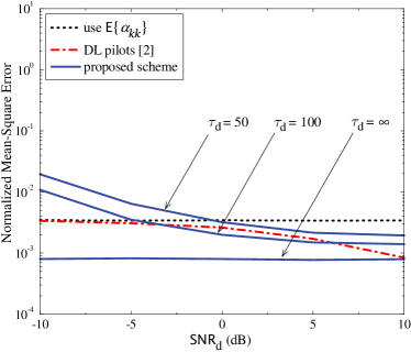
(a) Rayleigh fading channels

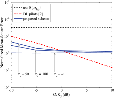
(b) Single-keyhole channels

Figure 2: Normalized MSE versus $\mathsf{SNR}_{\text{d}}$ for different channel estimation schemes, for MR processing. Here, $M=100$, $K=10$, and $\mathsf{SNR}_{\text{u}}=0$ dB.

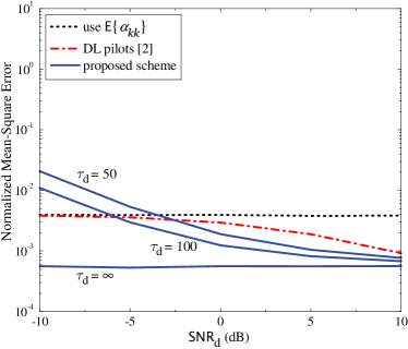
(a) Rayleigh fading channels

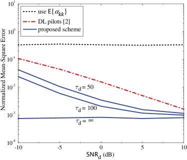
(b) Single-keyhole channels

Figure 3: Same as Figure 2, but for ZF processing.

Next we study the affects of the number of BS antennas and the number of keyholes on the performance of our proposed scheme. We choose $K=10$, $\tau_{\mathrm{d}}=100$, $\mathsf{SNR}_{\text{u}}=0$ dB, and $\mathsf{SNR}_{\text{d}}=5$ dB. Figure 4 shows the normalized MSE versus $M$ for different numbers of keyholes $n_{\tt KH}$ with MR and ZF processing. When $n_{\tt KH}=\infty$, we have Rayleigh fading. As expected, the MSE reduces when $M$ increases. More importantly, our proposed scheme works well even when $M$ is not large. Furthermore, we can see that the MSE does not change much when the number of keyholes varies. This implies the robustness of our proposed scheme against the different propagation environments.

Note that, with the beamforming training scheme in [2], we additionally have to spend at least $K$ symbols on training pilots (this is not accounted for here, since we only evaluate MSE). By contrast, our proposed scheme does not require any resources for downlink training. To account for the loss due to training, we will examine the net throughput in the next part.

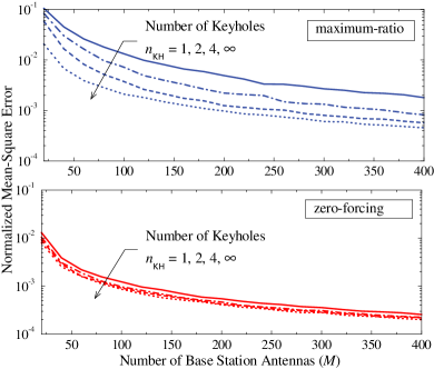
Figure 4: Normalized MSE versus $M$ for different number of keyholes $n_{k}=n_{\tt KH}$, using Algorithm 1. Here, $\mathsf{SNR}_{\text{u}}=0$ dB, $\mathsf{SNR}_{\text{d}}=5$ dB, and $K=10$.

VI-B Downlink Net Throughput

The downlink net throughputs of three cases—use $\mathsf{E}\left\{{\alpha_{kk}}\right\}$, DL pilots, and proposed schemes—are defined as:

$$\mathcal{S}_{k}^{\text{noCSI}} =B\frac{\tau_{\mathrm{d}}}{\tau_{\mathrm{c}}}R_{k}^{\text{noCSI}},$$ (50)

$$\mathcal{S}_{k}^{\text{pilot}} =B\frac{\tau_{\mathrm{d}}-\tau_{\mathrm{d,p}}}{\tau_{\mathrm{c}}}R_{k}^{\text{pilot}},$$ (51)

$$\mathcal{S}_{k}^{\text{blind}} =B\frac{\tau_{\mathrm{d}}}{\tau_{\mathrm{c}}}R_{k}^{\text{blind}},$$ (52)

where $B$ is the spectral bandwidth, $\tau_{\mathrm{c}}$ is again the coherence interval in symbols, and $\tau_{\mathrm{d}}$ is the number of symbols per coherence interval allocated for downlink transmission. Note that $R_{k}^{\text{noCSI}}$, $R_{k}^{\text{pilot}}$, and $R_{k}^{\text{blind}}$ are the corresponding achievable rates of these cases. $R_{k}^{\text{blind}}$ is given by (44), while $R_{k}^{\text{pilot}}$ and $R_{k}^{\text{noCSI}}$ can be computed by using (44), but $\hat{\hat{\alpha}}_{kk}(1)$ is replaced with the channel estimate of $\alpha_{kk}$ using scheme in [2] respectively $\mathsf{E}\left\{{\alpha_{kk}}\right\}$. The term $\dfrac{\tau_{\mathrm{d}}}{\tau_{\mathrm{c}}}$ in (50) and (52) comes from the fact that, for each coherence interval of $\tau_{\mathrm{c}}$ samples, with our proposed scheme and the case of no channel estimation, we spend $\tau_{\mathrm{d}}$ samples for downlink payload data transmission. The term $\dfrac{\tau_{\mathrm{d}}-\tau_{\mathrm{d,p}}}{\tau_{\mathrm{c}}}$ in (51) comes from the fact that we spend $\tau_{\mathrm{d,p}}$ symbols on downlink pilots to estimate the effect channel gains [2]. In all examples, we choose $B=20$ MHz and $\tau_{\mathrm{d}}=\tau_{\mathrm{c}}/2$ (half of the coherence interval is used for downlink transmission).

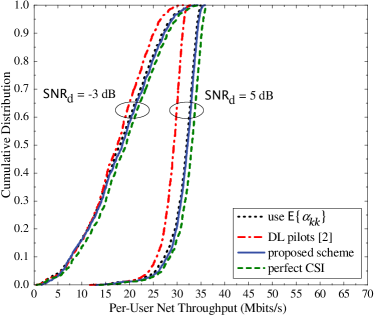
(a) Rayleigh fading channels

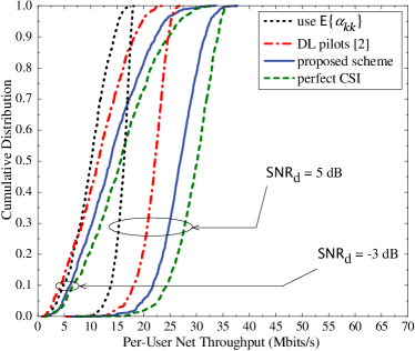
(b) Single-keyhole channels

Figure 5: The cumulative distribution of the per-user downlink net throughput for MR processing. Here, $M=100$, $K=10$, $\tau_{\mathrm{c}}=200$ ($\tau_{\mathrm{d}}=100$), $\mathsf{SNR}_{\text{d}}=10\mathsf{SNR}_{\text{u}}$, and $B=20$ MHz.

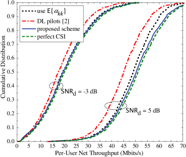
(a) Rayleigh fading channels

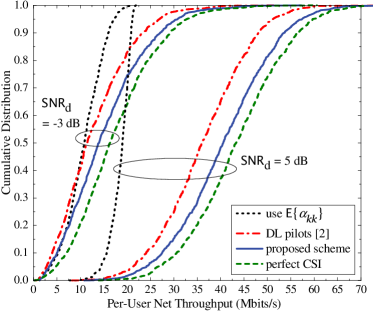
(b) Single-keyhole channels

Figure 6: Same as Figure 5, but for ZF processing.

We consider a more realistic scenario which incorporates the large-scale fading and max-min power control:

• To generate the large-scale fading, we consider an annulus-shaped cell with a radius of $R_{\text{max}}$ meters, and the BS is located at the cell center. $K+1$ users are placed uniformly at random in the cell with a minimum distance of $R_{\text{min}}$ meters from the BS. The user with the smallest large-scale fading $\beta_{k}$ is dropped, such that $K$ users remain. The large-scale fading is modeled by path loss, shadowing (with log-normal distribution), and random user locations:

  $$\beta_{k}=\text{PL}_{0}\left(\frac{d_{k}}{R_{\text{min}}}\right)^{\upsilon}\times 10^{\frac{\sigma_{\text{sh}}\cdot\mathcal{N}(0,1)}{10}},$$ (53)

  where $\upsilon$ is the path loss exponent and $\sigma_{\text{sh}}$ is the standard deviation of the shadow fading. The factor $\text{PL}_{0}$ in (53) is a reference path loss constant which is chosen to satisfy a given downlink cell-edge SNR, $\mathsf{SNR}_{\text{d}}$. In the simulation, we choose $R_{\text{min}}=100$, $R_{\text{max}}=1000$, $\upsilon=3.8$, and $\sigma_{\text{sh}}=8$ dB. We generate $1000$ random realizations of user locations and shadowing fading profiles.

• The power control control coefficients $\{\eta_{k}\}$ are chosen from the max-min power control algorithm [28]:

  $$\eta_{k}=\left\{\begin{array}[]{ll}\frac{1+\rho_{\mathrm{d}}\beta_{k}}{\rho_{\mathrm{d}}\gamma_{k}\left(\frac{1}{\rho_{\mathrm{d}}}\sum\limits_{k^{\prime}=1}^{K}\frac{1}{\gamma_{k^{\prime}}}+\sum\limits_{k^{\prime}=1}^{K}\frac{\beta_{k^{\prime}}}{\gamma_{k^{\prime}}}\right)},&\text{for MR,}\\ \frac{1+\rho_{\mathrm{d}}(\beta_{k}-\gamma_{k})}{\rho_{\mathrm{d}}\gamma_{k}\left(\frac{1}{\rho_{\mathrm{d}}}\sum\limits_{k^{\prime}=1}^{K}\frac{1}{\gamma_{k^{\prime}}}+\sum\limits_{k^{\prime}=1}^{K}\frac{\beta_{k^{\prime}}-\gamma_{k^{\prime}}}{\gamma_{k^{\prime}}}\right)},&\text{for ZF.}\\ \end{array}\right.$$ (56)

  This max-min power control offers uniformly good service for all users for the case where the $k$th user uses $\mathsf{E}\left\{{\alpha_{kk}}\right\}$ as estimate of $\alpha_{kk}$.

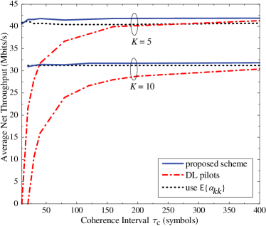
(a) Rayleigh fading channels

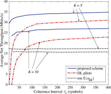
(b) Single-keyhole channels

Figure 7: The average per-user downlink net throughput for MR processing. Here, $M=100$, $\mathsf{SNR}_{\text{d}}=10\mathsf{SNR}_{\text{u}}=5$ dB, and $B=20$ MHz.

Figures 5 and 6 show the cumulative distributions of the per-user downlink net throughput for MR respectively ZF processing, under Rayleigh fading and single-keyhole channels. Here we choose $M=100$, $K=10$, $\tau_{\mathrm{c}}=200$, and $\mathsf{SNR}_{\text{d}}=10\mathsf{SNR}_{\text{u}}$. As a baseline for comparisons, we additionally add the curves labelled “perfect CSI”. These curves represent the presence of a genie receiver at the $k$th user, which knows the channel gain perfectly. For both propagation environments, our proposed scheme is the best and performs very close to the genie receiver. For Rayleigh fading channels, due to the hardening property of the channels, our proposed scheme and the scheme using statistical property of the channels are comparable. These schemes perform better than the beamforming training scheme in [2]. The reason is that, with beamforming training scheme, we have to spend $\tau_{\mathrm{d,p}}$ pilot samples for the downlink training. For single-keyhole channels, the channels do not harden, and hence, it is necessary to estimate the effective channel gains. Our proposed scheme improves the system performance significantly. At $\mathsf{SNR}_{\text{d}}=5$ dB, with MR processing, our proposed scheme can improve the 95%-likely net throughput by about $20$% and $60$%, compared with the downlink beamforming training scheme respectively the case of without channel estimation. With ZF processing, our proposed scheme can improve the 95%-likely net throughput by $15$% and $66$%, respectively. The MSE of “use $\mathsf{E}\left\{{\alpha_{kk}}\right\}$” does not depend on $\mathsf{SNR}_{\text{d}}$ (see Figures 2 and 3), but it depends on $\mathsf{SNR}_{\text{u}}$. In Figures 5 and 6, when $\mathsf{SNR}_{\text{d}}$ increases, $\mathsf{SNR}_{\text{u}}$ also increases, and hence, the per-user throughput gaps between the “use $\mathsf{E}\left\{{\alpha_{kk}}\right\}$” curves and the “perfect CSI” curves vary as $\mathsf{SNR}_{\text{d}}$ increases.

Finally, we investigate the effect of the coherence interval $\tau_{\mathrm{c}}$ and the number of users $K$ on the performance of our proposed scheme. Figure 7 shows the average downlink net throughput versus $\tau_{\mathrm{c}}$ with MR processing for different $K$ in both Rayleigh fading and keyhole channels. The average is taken over the large-scale fading. Our proposed scheme overcomes the disadvantage of beamforming training scheme in high mobility environments (short coherence interval), and the disadvantage of statistical property-based scheme in non-hardening propagation environments, and hence, performs very well in many cases, even when $\tau_{\mathrm{c}}$ and $K$ are small.

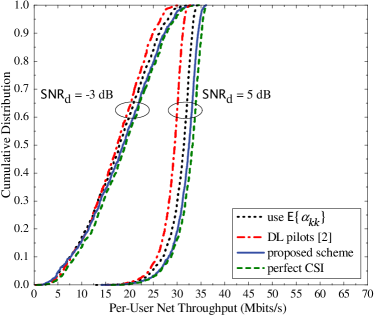
(a) Rayleigh fading channels

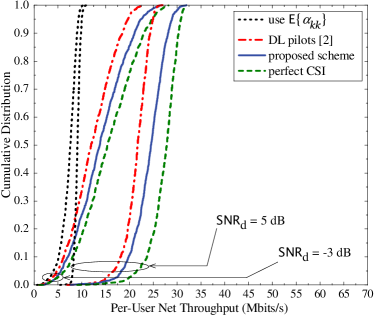
(b) Single-keyhole channels

Figure 8: Same as Figure 5, but with long-term average power constraint (57).

VII Comments

VII-A Short-Term V.s. Long-Term Average Power Constraint

The precoding vectors ${\mathbf{a}}_{k}$ in (8) and (9) are chosen to satisfy a short-term average power constraint where the expectation of (6) is taken over only ${\mathbf{s}}(n)$. This short-term average power constraint is not the only possibility. Alternatively, one could consider a long-term average power constraint where the expectation in (6) is taken over ${\mathbf{s}}(n)$ and over the small-scale fading. With MR combining, the long-term-average-power-based precoding vectors $\{{\mathbf{a}}_{k}\}$ are

$${\mathbf{a}}_{k}=\frac{\hat{{\mathbf{g}}}_{k}}{\sqrt{\mathsf{E}\left\{{\|\hat{{\mathbf{g}}}_{k}\|^{2}}\right\}}}=\frac{\hat{{\mathbf{g}}}_{k}}{\sqrt{M\gamma_{k}}},\quad k=1,\ldots,K.$$ (57)

However, with ZF, the long-term-average-power-based precoder is not always valid. For example, for single-keyhole channels, perfect uplink estimation, and $K=1$, we have

$$\mathsf{E}\left\{{\left\|\left[{\mathbf{G}}\left({\mathbf{G}}^{H}{\mathbf{G}}\right)^{-1}\right]_{k}\right\|^{2}}\right\},$$ (58)

which is infinite.

We emphasize here that compared to the short-term average power case, the long-term average power case does not make a difference in the sense that the resulting effective channel gain does not always harden, and hence, it needs to be estimated. (The harding property of the channels is discussed in detail in Section III.) To see this more quantitatively, we compare the performance of three cases: “use $\mathsf{E}\left\{{\alpha_{kk}}\right\}$”, “DL pilots [2]”, and “proposed scheme” for MR with long-term average power constraint (57). As seen in Figure 8, under keyhole channels, our proposed scheme improves the net throughput significantly, compared to the “use $\mathsf{E}\left\{{\alpha_{kk}}\right\}$” case.

VII-B Flaw of the Bound in [2, 11]

In the above numerical results, the curves with downlink pilots are obtained by first replacing $\hat{\hat{\alpha}}_{kk}(1)$ in (44) with the channel estimate obtained using the algorithm in [2], and then using the numerical technique discussed in Remark 2 to compute the capacity bound.

Closed-form expressions for achievable rates with downlink training were given in [2, Eq. (12)] and [11]. However, those formulas were not rigorously correct, since $\{a_{kk^{\prime}}\}$ are non-Gaussian in general (even in Rayleigh fading) and hence the linear MMSE estimate is not equal to the MMSE estimate; the expressions for the capacity bounds in [2, 11] are valid only when the MMSE estimate is inserted. However, the expressions [2, 11] are likely to be extremely accurate approximations. A similar approximation was stated in [12].

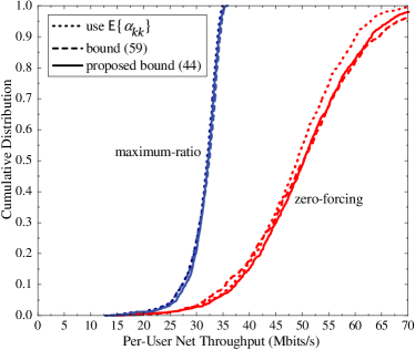
(a) Rayleigh fading channels

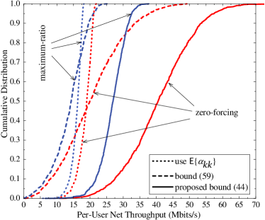
(b) Single-keyhole channels

Figure 9: The cumulative distribution of the per-user downlink net throughput for MR and ZF processing. Here, $M=100$, $K=10$, $\tau_{\mathrm{c}}=200$ ($\tau_{\mathrm{d}}=100$), $\mathsf{SNR}_{\text{d}}=10\mathsf{SNR}_{\text{u}}=5$ dB, and $B=20$ MHz.

VII-C Using the Capacity Bounding Technique of [8, 10]

It may be tempting to use the bounding technique in [8, 10] to derive a simpler capacity bound as follows (the index $n$ is omitted for simplicity of notation):

• Divide the received signal $\eqref{eq:sys3}$ by the channel estimate $\hat{\hat{\alpha}}_{kk}$,

  $$y^{\prime}_{k} =\frac{y_{k}}{\sqrt{\rho_{\mathrm{d}}\eta_{k}}\hat{\hat{\alpha}}_{kk}}$$

  $$=\frac{\alpha_{kk}}{\hat{\hat{\alpha}}_{kk}}s_{k}+\sum_{k^{\prime}\neq k}^{K}\sqrt{\frac{\eta_{k^{\prime}}}{\eta_{k}}}\frac{\alpha_{kk^{\prime}}}{\hat{\hat{\alpha}}_{kk}}s_{k^{\prime}}+\frac{w_{k}}{\sqrt{\rho_{\mathrm{d}}\eta_{k}}\hat{\hat{\alpha}}_{kk}}.$$ (59)

• Rewrite (i)) as the sum of the desired signal multiplied with a deterministic gain, $\mathsf{E}\left\{{\frac{\alpha_{kk}}{\hat{\hat{\alpha}}_{kk}}}\right\}s_{k}$, and remaining terms which constitute uncorrelated effective noise,

  $$y^{\prime}_{k} =\mathsf{E}\left\{{\frac{\alpha_{kk}}{\hat{\hat{\alpha}}_{kk}}}\right\}s_{k}+\left(\frac{\alpha_{kk}}{\hat{\hat{\alpha}}_{kk}}-\mathsf{E}\left\{{\frac{\alpha_{kk}}{\hat{\hat{\alpha}}_{kk}}}\right\}\right)s_{k}$$

  $$+\sum_{k^{\prime}\neq k}^{K}\sqrt{\frac{\eta_{k^{\prime}}}{\eta_{k}}}\frac{\alpha_{kk^{\prime}}}{\hat{\hat{\alpha}}_{kk}}s_{k^{\prime}}+\frac{w_{k}}{\sqrt{\rho_{\mathrm{d}}\eta_{k}}\hat{\hat{\alpha}}_{kk}}.$$ (60)

$$R_{k}^{\text{UnF}}=\log_{2}\left(1+\frac{\left|\mathsf{E}\left\{{\frac{\alpha_{kk}}{\hat{\hat{\alpha}}_{kk}}}\right\}\right|^{2}}{\operatorname{\mathsf{Var}}\left\{{\frac{\alpha_{kk}}{\hat{\hat{\alpha}}_{kk}}}\right\}+\sum\limits_{k^{\prime}\neq k}^{K}\frac{\eta_{k^{\prime}}}{\eta_{k}}\mathsf{E}\left\{{\left|\frac{\alpha_{kk^{\prime}}}{\hat{\hat{\alpha}}_{kk}}\right|^{2}}\right\}+\frac{1}{\rho_{\mathrm{d}}\eta_{k}}\mathsf{E}\left\{{\frac{1}{\left|\hat{\hat{\alpha}}_{kk}\right|^{2}}}\right\}}\right).$$ (59)

The worst-case Gaussian noise property [26] then yields the capacity bound (59), shown at the top of the next page. This bound does not require the complicated numerical computation given in Section V. However, this bound is tight only when the effective channel gain $\alpha_{kk}$ hardens, which is generally not the case under the models that we consider herein.

More quantitatively, Figure 9 shows a comparison between our new bound (44) and the bound (59). The figure shows the cumulative distributions of the per-user downlink net throughput for MR and ZF processing, for the same setup as in Section VI-B. In Rayleigh fading, the throughputs for the three cases “use $\mathsf{E}\left\{{\alpha_{kk}}\right\}$”, “bound (59)”, and “proposed bound (44)”, are very close, and hence, relying on statistical channel knowledge ($\mathsf{E}\left\{{\alpha_{kk}}\right\})$ for signal detection is good enough – obviating the need for the bound in (59). In in keyhole channels, the bound (59) is significantly inferior to our proposed bound. Therefore, the bound (59) is of no use neither in Rayleigh fading nor in keyhole channels.

VIII Conclusion

In the Massive MIMO downlink, in propagation environments where the channel hardens, using the mean of the effective channel gain for signal detection is good enough. However, the channels may not always harden. Then, to reliably decode the transmitted signals, each user should estimate its effective channel gain rather than approximate it by its mean. We proposed a new blind channel estimation scheme at the users which does not require any downlink pilots. With this scheme, the users can blindly estimate their effective channel gains directly from the data received during a coherence interval. Our proposed channel estimation scheme is computationally easy, and performs very well. Numerical results show that in non-hardening propagation environments and for large numbers of BS antennas, our proposed scheme significantly outperforms both the downlink beamforming training scheme in [2] and the conventional approach that approximates the effective channel gains by their means.

-A Derivation of (III-C2)

We have,

$$\frac{\operatorname{\mathsf{Var}}\left\{{{\left\|{\mathbf{g}}_{k}\right\|^{2}}}\right\}}{\left(\mathsf{E}\left\{{{\left\|{\mathbf{g}}_{k}\right\|^{2}}}\right\}\right)^{2}}\!=\!\frac{1}{\beta_{k}^{2}M^{2}}\mathsf{E}\left\{{\left\|{\mathbf{g}}_{k}\right\|^{4}}\right\}-\frac{1}{\beta_{k}^{2}M^{2}}\!\left(\!\mathsf{E}\left\{{\left\|{\mathbf{g}}_{k}\right\|^{2}}\right\}\right)^{2}$$

$$=\frac{1}{\beta_{k}^{2}M^{2}}\mathsf{E}\left\{{\left\|{\mathbf{g}}_{k}\right\|^{4}}\right\}-1$$

$$=\frac{1}{M^{2}}\mathsf{E}\left\{{\left|\sum_{i=1}^{n_{k}}\sum_{n=1}^{n_{k}}\left(c_{i}^{(k)}a_{i}^{(k)}{\mathbf{b}}_{i}^{(k)}\right)^{H}c_{n}^{(k)}a_{n}^{(k)}{\mathbf{b}}_{n}^{(k)}\right|^{2}}\right\}-1$$

$$=\frac{1}{M^{2}}\mathsf{E}\left\{{\left|\sum_{i=1}^{n_{k}}\!\left\|\tilde{{\mathbf{b}}}_{i}^{(k)}\right\|^{2}\!+\!\sum_{i=1}^{n_{k}}\!\sum_{n\neq i}^{n_{k}}\!\left(\tilde{{\mathbf{b}}}_{i}^{(k)}\right)^{H}\!\tilde{{\mathbf{b}}}_{n}^{(k)}\right|^{2}}\right\}\!-\!1,$$ (60)

where $\tilde{{\mathbf{b}}}_{i}^{(k)}\triangleq c_{i}^{(k)}a_{i}^{(k)}{\mathbf{b}}_{i}^{(k)}$. We can see that, the terms in the double sum have zero mean. We now consider the covariance between two arbitrary terms:

$$\mathsf{E}\left\{{\left(\tilde{{\mathbf{b}}}_{i}^{(k)}\right)^{H}\tilde{{\mathbf{b}}}_{n}^{(k)}\left(\left(\tilde{{\mathbf{b}}}_{i^{\prime}}^{(k)}\right)^{H}\tilde{{\mathbf{b}}}_{n^{\prime}}^{(k)}\right)^{\ast}}\right\},$$

where $i\neq n$, $i^{\prime}\neq n^{\prime}$, and $(i,n)\neq(i^{\prime},n^{\prime})$. Clearly, if $(i,n)\neq(n^{\prime},i^{\prime})$, then

$$\mathsf{E}\left\{{\left(\tilde{{\mathbf{b}}}_{i}^{(k)}\right)^{H}\tilde{{\mathbf{b}}}_{n}^{(k)}\left(\left(\tilde{{\mathbf{b}}}_{i^{\prime}}^{(k)}\right)^{H}\tilde{{\mathbf{b}}}_{n^{\prime}}^{(k)}\right)^{\ast}}\right\}=0.$$

If $(i,n)=(n^{\prime},i^{\prime})$, the we have

$$\mathsf{E}\left\{{\left(\tilde{{\mathbf{b}}}_{i}^{(k)}\right)^{H}\tilde{{\mathbf{b}}}_{n}^{(k)}\left(\left(\tilde{{\mathbf{b}}}_{i^{\prime}}^{(k)}\right)^{H}\tilde{{\mathbf{b}}}_{n^{\prime}}^{(k)}\right)^{\ast}}\right\}$$

$$=\mathsf{E}\left\{{\left(\tilde{{\mathbf{b}}}_{i}^{(k)}\right)^{H}\tilde{{\mathbf{b}}}_{n}^{(k)}\left(\tilde{{\mathbf{b}}}_{n}^{(k)}\right)^{T}\left(\tilde{{\mathbf{b}}}_{i}^{(k)}\right)^{\ast}}\right\}=0,$$ (61)

where we used the fact that if $z$ is a circularly symmetric complex Gaussian random variable with zero mean, then $\mathsf{E}\left\{{z^{2}}\right\}=0$. The above result implies that the terms $\left(\tilde{{\mathbf{b}}}_{i}^{(k)}\right)^{H}\tilde{{\mathbf{b}}}_{n}^{(k)}$ [inside the double sum of (-A)] are zero-mean mutual uncorrelated random variables. Furthermore, they are uncorrelated with $\sum_{i=1}^{n_{k}}\left\|\tilde{{\mathbf{b}}}_{i}^{(k)}\right\|^{2}$, so (-A) can be rewritten as:

$$\frac{\operatorname{\mathsf{Var}}\left\{{{\left\|{\mathbf{g}}_{k}\right\|^{2}}}\right\}}{\left(\mathsf{E}\left\{{{\left\|{\mathbf{g}}_{k}\right\|^{2}}}\right\}\right)^{2}} =\frac{1}{M^{2}}\underbrace{\mathsf{E}\left\{{\left|\sum_{i=1}^{n_{k}}\left\|\tilde{{\mathbf{b}}}_{i}^{(k)}\right\|^{2}\right|^{2}}\right\}}_{\triangleq\text{Term1}}$$

$$+\frac{1}{M^{2}}\sum_{i=1}^{n_{k}}\sum_{n\neq i}^{n_{k}}\underbrace{\mathsf{E}\left\{{\left|\left(\tilde{{\mathbf{b}}}_{i}^{(k)}\right)^{H}\tilde{{\mathbf{b}}}_{n}^{(k)}\right|^{2}}\right\}}_{\triangleq\text{Term2}}-1.$$ (62)

We have,

Term1 $$=\sum_{i=1}^{n_{k}}\mathsf{E}\left\{{\left\|\tilde{{\mathbf{b}}}_{i}^{(k)}\right\|^{4}}\right\}+\sum_{i=1}^{n_{k}}\sum_{n\neq i}^{n_{k}}\mathsf{E}\left\{{\left\|\tilde{{\mathbf{b}}}_{i}^{(k)}\right\|^{2}\left\|\tilde{{\mathbf{b}}}_{n}^{(k)}\right\|^{2}}\right\}$$

$$=\sum_{i=1}^{n_{k}}\mathsf{E}\left\{{\left|c_{i}^{(k)}\right|^{4}\left|a_{i}^{(k)}\right|^{4}\left\|{{\mathbf{b}}}_{i}^{(k)}\right\|^{4}}\right\}$$

$$+\sum_{i=1}^{n_{k}}\!\sum_{n\neq i}^{n_{k}}\!\mathsf{E}\left\{{\!\left|c_{i}^{(k)}\!\right|^{2}\!\left|a_{i}^{(k)}\right|^{2}\left\|{{\mathbf{b}}}_{i}^{(k)}\right\|^{2}\!}\right\}\!\mathsf{E}\left\{{\!\left|c_{n}^{(k)}\!\right|^{2}\left|a_{n}^{(k)}\right|^{2}\!\left\|{{\mathbf{b}}}_{n}^{(k)}\right\|^{2}\!}\right\}$$

$$=2M(M+1)\sum_{i=1}^{n_{k}}\left|c_{i}^{(k)}\right|^{4}+M^{2}\sum_{i=1}^{n_{k}}\sum_{n\neq i}^{n_{k}}\left|c_{i}^{(k)}\right|^{2}\left|c_{n}^{(k)}\right|^{2}$$

$$=M(M+2)\sum_{i=1}^{n_{k}}\left|c_{i}^{(k)}\right|^{4}+M^{2},$$ (63)

where we have used the identity that if ${\mathbf{z}}\sim\mathcal{CN}\left({\mathbf{0}},{{\mathbf{I}}_{n}}\right)$, then $\mathsf{E}\left\{{\left\|{\mathbf{z}}\right\|^{4}}\right\}=n(n+1)$.

Furthermore, we have

$$\text{Term2}=\mathsf{E}\left\{{\left|\left(c_{i}^{(k)}a_{i}^{(k)}{\mathbf{b}}_{i}^{(k)}\right)^{H}c_{n}^{(k)}a_{n}^{(k)}{\mathbf{b}}_{n}^{(k)}\right|^{2}}\right\}$$

$$=\left|c_{i}^{(k)}\right|^{2}\left|c_{n}^{(k)}\right|^{2}\operatorname{\mathsf{E}}{\left|a_{i}^{(k)}\right|^{2}}\mathsf{E}\left\{{\left|a_{n}^{(k)}\right|^{2}}\right\}\operatorname{\mathsf{E}}{\left|\left({\mathbf{b}}_{i}^{(k)}\right)^{H}{\mathbf{b}}_{n}^{(k)}\right|^{2}}$$

$$=M\left|c_{i}^{(k)}\right|^{2}\left|c_{n}^{(k)}\right|^{2}.$$ (64)

Substituting (-A) and (-A) into (-A), we obtain

$$\frac{\operatorname{\mathsf{Var}}\left\{{{\left\|{\mathbf{g}}_{k}\right\|^{2}}}\right\}}{\left(\mathsf{E}\left\{{{\left\|{\mathbf{g}}_{k}\right\|^{2}}}\right\}\right)^{2}} =\left(1+\frac{1}{M}\right)\sum_{i=1}^{n_{k}}\left|c_{i}^{(k)}\right|^{4}+\frac{1}{M}.$$ (65)

-B Derivation of (43)

Here, we provide the proof of (43).

• With MR, for both Rayleigh and keyhole channels, ${\mathbf{g}}_{k}$ and ${\mathbf{a}}_{k^{\prime}}$ are independent, for $k\neq k^{\prime}$. Thus, we have

  $$\mathsf{E}\left\{{|\alpha_{kk^{\prime}}|^{2}}\right\} =\mathsf{E}\left\{{{\mathbf{a}}_{k^{\prime}}^{H}{\mathbf{g}}_{k}{\mathbf{g}}_{k}^{H}{\mathbf{a}}_{k^{\prime}}}\right\}$$

  $$=\beta_{k}\mathsf{E}\left\{{\left\|{\mathbf{a}}_{k^{\prime}}\right\|^{2}}\right\}$$

  $$=\beta_{k}.$$ (66)

• With ZF, for Rayleigh channels, the channel estimate $\hat{{\mathbf{g}}}_{k}$ is independent of the channel estimation error $\tilde{{\mathbf{g}}}_{k}$. So $\tilde{{\mathbf{g}}}_{k}$ and ${\mathbf{a}}_{k^{\prime}}$ are independent. In addition, from (9), we have

  $$\hat{{\mathbf{g}}}_{k}^{H}{\mathbf{a}}_{k^{\prime}}=0,\quad k\neq k^{\prime},$$

  and therefore,

  $$\mathsf{E}\left\{{|\alpha_{kk^{\prime}}|^{2}}\right\} =\mathsf{E}\left\{{|{\mathbf{g}}_{k}^{H}{\mathbf{a}}_{k^{\prime}}|^{2}}\right\}$$

  $$=\mathsf{E}\left\{{|\tilde{{\mathbf{g}}}_{k}^{H}{\mathbf{a}}_{k^{\prime}}|^{2}}\right\}$$

  $$=\mathsf{E}\left\{{{\mathbf{a}}_{k^{\prime}}^{H}\tilde{{\mathbf{g}}}_{k}\tilde{{\mathbf{g}}}_{k}^{H}{\mathbf{a}}_{k^{\prime}}}\right\}$$

  $$=(\beta_{k}-\gamma_{k})\mathsf{E}\left\{{\left\|{\mathbf{a}}_{k^{\prime}}\right\|^{2}}\right\}$$

  $$=\beta_{k}-\gamma_{k}.$$ (67)

Hien Quoc Ngo received the B.S. degree in electrical engineering from Ho Chi Minh City University of Technology, Vietnam, in 2007. He then received the M.S. degree in Electronics and Radio Engineering from Kyung Hee University, Korea, in 2010, and the Ph.D. degree in communication systems from Linköping University (LiU), Sweden, in 2015. From May to December 2014, he visited Bell Laboratories, Murray Hill, New Jersey, USA. Hien Quoc Ngo is currently a postdoctoral researcher of the Division for Communication Systems in the Department of Electrical Engineering (ISY) at Linköping University, Sweden. He is also a Visiting Research Fellow at the School of Electronics, Electrical Engineering and Computer Science, Queen’s University Belfast, U.K. His current research interests include massive (large-scale) MIMO systems and cooperative communications. Dr. Hien Quoc Ngo received the IEEE ComSoc Stephen O. Rice Prize in Communications Theory in 2015. He also received the IEEE Sweden VT-COM-IT Joint Chapter Best Student Journal Paper Award in 2015. He was an IEEE Communications Letters exemplary reviewer for 2014, an IEEE Transactions on Communications exemplary reviewer for 2015. He has been a member of Technical Program Committees for several IEEE conferences such as ICC, Globecom, WCNC, VTC, WCSP, ISWCS, ATC, ComManTel.

Erik G. Larsson is Professor of Communication Systems at Linköping University (LiU) in Linköping, Sweden. He previously worked for the Royal Institute of Technology (KTH) in Stockholm, Sweden, the University of Florida, USA, the George Washington University, USA, and Ericsson Research, Sweden. In 2015 he was a Visiting Fellow at Princeton University, USA, for four months. He received his Ph.D. degree from Uppsala University, Sweden, in 2002. His main professional interests are within the areas of wireless communications and signal processing. He has co-authored some 130 journal papers on these topics, he is co-author of the two Cambridge University Press textbooks Space-Time Block Coding for Wireless Communications (2003) and Fundamentals of Massive MIMO (2016). He is co-inventor on 16 issued and many pending patents on wireless technology. He served as Associate Editor for, among others, the IEEE Transactions on Communications (2010-2014) and IEEE Transactions on Signal Processing (2006-2010). He serves as chair of the IEEE Signal Processing Society SPCOM technical committee in 2015–2016 and he served as chair of the steering committee for the IEEE Wireless Communications Letters in 2014–2015. He was the General Chair of the Asilomar Conference on Signals, Systems and Computers in 2015, and Technical Chair in 2012. He received the IEEE Signal Processing Magazine Best Column Award twice, in 2012 and 2014, and the IEEE ComSoc Stephen O. Rice Prize in Communications Theory in 2015. He is a Fellow of the IEEE.

References

- [1] H. Q. Ngo and E. G. Larsson, “Blind estimation of effective downlink channel gains in massive MIMO,” in Proc. IEEE International Conference on Acoustics, Speech and Signal Processing (ICASSP), Brisbane, Australia, Apr. 2015.
- [2] H. Q. Ngo, E. G. Larsson, and T. L. Marzetta, “Massive MU-MIMO downlink TDD systems with linear precoding and downlink pilots,” in Proc. Allerton Conference on Communication, Control, and Computing, Urbana-Champaign, Illinois, Oct. 2013.
- [3] E. G. Larsson, F. Tufvesson, O. Edfors, and T. L. Marzetta, “Massive MIMO for next generation wireless systems,” IEEE Commun. Mag., vol. 52, no. 2, pp. 186–195, Feb. 2014.
- [4] L. Lu, G. Y. Li, A. L. Swindlehurst, A. Ashikhmin, and R. Zhang, “An overview of massive MIMO: Benefits and challenges,” IEEE J. Select. Topics Signal Process., vol. 8, no. 5, pp. 742–758, Oct. 2014.
- [5] T. Bogale and L. B. Le, “Massive MIMO and mmWave for 5G wireless HetNet: Potentials and challenges,” IEEE Veh. Technol. Mag., vol. 11, no. 1, pp. 64–75, Feb. 2016.
- [6] X. Gao, O. Edfors, F. Rusek, and F. Tufvesson, “Massive MIMO performance evaluation based on measured propagation data,” IEEE Trans. Wireless Commun., vol. 14, no. 7, pp. 3899–3911, Jul. 2015.
- [7] Q. Zhang, S. Jin, K.-K. Wong, H. Zhu, and M. Matthaiou, “Power scaling of uplink massive MIMO systems with arbitrary-rank channel means,” IEEE J. Select. Topics Signal Process., vol. 8, no. 5, pp. 966–981, Oct. 2014.
- [8] J. Jose, A. Ashikhmin, T. L. Marzetta, and S. Vishwanath, “Pilot contamination and precoding in multi-cell TDD systems,” IEEE Trans. Wireless Commun., vol. 10, no. 8, pp. 2640–2651, Aug. 2011.
- [9] H. Yang and T. L. Marzetta, “Performance of conjugate and zero-forcing beamforming in large-scale antenna systems,” IEEE J. Sel. Areas Commun., vol. 31, no. 2, pp. 172–179, Feb. 2013.
- [10] J. Hoydis, S. ten Brink, and M. Debbah, “Massive MIMO in the UL/DL of cellular networks: How many antennas do we need?” IEEE J. Sel. Areas Commun., vol. 31, no. 2, pp. 160–171, Feb. 2013.
- [11] J. Zuo, J. Zhang, C. Yuen, W. Jiang, and W. Luo, “Multi-cell multi-user massive MIMO transmission with downlink training and pilot contamination precoding,” IEEE Trans. Veh. Technol., vol. 65, no. 8, pp. 6301–6314, Aug. 2016.
- [12] A. Khansefid and H. Minn, “Achievable downlink rates of MRC and ZF precoders in massive MIMO with uplink and downlink pilot contamination,” IEEE Trans. Commun., vol. 63, no. 12, pp. 4849–4864, Dec. 2015.
- [13] T. Kim, K. Min, and S. Choi, “Study on effect of training for downlink massive MIMO systems with outdated channel,” in Proc. IEEE International Conference on Communications (ICC), London, UK, Jun. 2015.
- [14] H. Q. Ngo, E. G. Larsson, and T. L. Marzetta, “Energy and spectral efficiency of very large multiuser MIMO systems,” IEEE Trans. Commun., vol. 61, no. 4, pp. 1436–1449, Apr. 2013.
- [15] P. Viswanath and D. N. C. Tse, “Sum capacity of the vector Gaussian broadcast channel and uplink-downlink duality,” IEEE Trans. Inf. Theory, vol. 49, no. 8, pp. 1912–1921, Aug. 2003.
- [16] H. Q. Ngo, E. G. Larsson, and T. L. Marzetta, “Aspects of favorable propagation in massive MIMO,” in Proc. European Signal Processing Conf. (EUSIPCO), Lisbon, Portugal, Sep. 2014.
- [17] Y.-G. Lim, C.-B. Chae, and G. Caire, “Performance analysis of massive MIMO for cell-boundary users,” IEEE Trans. Wireless Commun., vol. 14, no. 12, pp. 6827–6842, Dec. 2015.
- [18] A. L. Moustakas, H. U. Baranger, L. Balents, A. M. Sengupta, and S. H. Simon, “Communication through a diffusive medium: Coherence and capacity,” Science, vol. 287, no. 5451, pp. 287–290, 2000.
- [19] A. M. Tulino and S. Verdú, “Random matrix theory and wireless communications,” Foundations and Trends in Communications and Information Theory, vol. 1, no. 1, pp. 1–182, Jun. 2004.
- [20] D. Gesbert, H. Bölcskei, D. A. Gore, and A. J. Paulraj, “Outdoor MIMO wireless channels: Models and performance prediction,” IEEE Trans. Commun., vol. 50, no. 12, pp. 1926–1934, Dec. 2002.
- [21] P. Almers, F. Tufvensson, and A. F. Molisch, “Keyhole effect in MIMO wireless channels: Measurements and theory,” IEEE Trans. Wireless Commun., vol. 5, no. 12, pp. 3596–3604, Dec. 2006.
- [22] X. Li, S. Jin, X. Gao, and M. R. McKay, “Capacity bounds and low complexity transceiver design for double-scattering MIMO multiple access channels,” IEEE Trans. Signal Process., vol. 58, no. 5, pp. 2809–2822, May 2010.
- [23] C. Zhong, S. Jin, K.-K. Wong, and M. R. McKay, “Ergodic mutual information analysis for multi-keyhole MIMO channels,” IEEE Trans. Wireless Commun., vol. 10, no. 6, pp. 1754–1763, Jun. 2011.
- [24] G. Levin and S. Loyka, “From multi-keyholes to measure of correlation and power imbalance in MIMO channels: Outage capacity analysis,” IEEE Trans. Inf. Theory, vol. 57, no. 6, pp. 3515–3529, Jun. 2011.
- [25] T. M. Cover and J. A. Thomas, Elements of Information Theory. New York: Wiley, 1991.
- [26] M. Médard, “The effect upon channel capacity in wireless communications of perfect and imperfect knowledge of the channel,” IEEE Trans. Inf. Theory, vol. 46, no. 3, pp. 933–946, May 2000.
- [27] E. Björnson, E. G. Larsson, and T. L. Marzetta, “Massive MIMO: 10 myths and one critical question,” IEEE Commun. Mag., vol. 54, no. 2, pp. 114–123, Feb. 2016.
- [28] H. Yang and T. L. Marzetta, “A macro cellular wireless network with uniformly high user throughputs,” in Proc. IEEE Veh. Technol. Conf. (VTC), Sep. 2014.