The Oslo model, hyperuniformity, and the quenched Edwards-Wilkinson model

Abstract

We present simulations of the 1-dimensional Oslo rice pile model in which the critical height at each site is randomly reset after each toppling. We use the fact that the stationary state of this sandpile model is hyperuniform to reach system of sizes $>10^{7}$. Most previous simulations were seriously flawed by important finite size corrections. We find that all critical exponents have values consistent with simple rationals: $\nu=4/3$ for the correlation length exponent, $D=9/4$ for the fractal dimension of avalanche clusters, and $z=10/7$ for the dynamical exponent. In addition we relate the hyperuniformity exponent to the correlation length exponent $\nu$. Finally we discuss the relationship with the quenched Edwards-Wilkinson (qEW) model, where we find in particular that the local roughness exponent is $\alpha_{\rm loc}=1$.

I Introduction

Although self-organized critical (SOC) sandpile models Bak:1987 ; Ivash:1994 ; Ktit:2000 ; ddrev ; redig ; propp have been studied intensively during the last thirty years, many of their aspects are still not well understood. For example, the critical exponents of avalanche distributions in the original Bak-Tang-Wiesenfeld sandpile model, on the square lattice, are still not known. The question of universality classes of different sandpile models is also not well understood Benhur ; Tebaldi:1999 . It is realized that models with stochastic toppling rules Manna ; Oslo ; Zhang ; Maslov-Zhang ; Rossi ; Mohanty:2002 ; Mohanty:2007 are in a different universality class than those with deterministic toppling rules. In particular, strong indications were found in BBBMH that models with stochastic toppling rules and with continuous local stresses (sandpile heights) behave differently from those with discrete ones. On the other hand, as already noted by Tang and Bak Tang ; Tang2 ; Grass-Manna , for all these models exist also non-self organized versions, now called fixed-energy sandpiles, that should show conventional (co-dimension one) critical points. The fixed-energy sandpiles (FES) undergo an active-absorbing state transition as a function of the mean density of particles. An important question has been if this transition is in the universality class of directed percolation. This question is not clearly understood yet Manna ; Oslo ; Zhang ; Maslov-Zhang ; Rossi ; Mohanty:2002 ; Mohanty:2007 . In FES, the number of absorbing states grows exponentially with the size of system. This alone would not create a problem, as it is known that models with many absorbing states can still be in the DP universality class – provided they do not have too-long-ranged correlations Hinrichsen .

One problem in numerical studies is precisely the long-ranged correlations in the absorbing states at criticality, called in the following “natural critical states” (NCS). A straightforward strategy seems to consist in studying states remaining after large avalanches have died, in systems poised to the critical point. But this is not possible, since it is not feasible to wait until avalanches die on very large systems (the average CPU time per avalanche diverges with system size). Thus one has to do some tricks that – unless one is sufficiently careful – can introduce spurious correlations in the NCS. While this problem was known quite early footnote3 , the first papers that tried to deal with it carefully and systematically Mohanty:2002 ; Mohanty:2007 ; BBBMH were published rather recently. They indicated that there exists in fact a universality class of stochastic sandpile models, but it seemed to be identical with the DP universality class. In fact, two of us have given heuristic arguments earlier, but no proof Mohanty:2002 ; Mohanty:2007 , that stochastic sandpile models in the Manna universality class will flow into the DP universality class if we add an appropriate perturbation.

It is the purpose of the present paper to clarify the situation somewhat. We study in detail the one-dimensional Oslo model oslo1 , which is one of the simplest nontrivial stochastic sandpile models. It has stochasticity in the toppling rules, and the critical height at each site is randomly reset after each toppling. Thus, it may be said that there is a degree of ”stickiness” in the model. While the model has some interesting properties due to its unusual algebraic structure, its steady state and critical properties are not known exactly so far ddoslo . We will study the behavior of other directed Oslo-type sandpile models on the 2-dimensional square lattice in a forthcoming paper. Here we study the 1-dimensional Oslo model using numerical simulations of much larger systems (and with much higher statistics) than what had been possible previously. As we said, simulations of FES at the critical point are hampered by the difficulty of sampling from the correct NCS. On the other hand, precise simulations of the SOC versions are difficult, because the open boundary conditions lead to large finite-size corrections, unless one can simulate huge systems. The latter, however, is made difficult by very long transients (during which the proper NCS has to build up). As a consequence, the largest published simulations of the 1-$d$ Oslo model are for systems of size $\approx 20,000$. Without the transients, systems larger by one or two units of magnitude would be easy to simulate on modern computers.

Our large-scale simulations are made possible by two technical improvements: (i) We use a new method of triggering avalanches in the FES that preserves all NCS correlations; (ii) We use initial configurations which are close to NCS configurations to reduce the time required to reach the NCS state.

Crucial for the latter is the observation, made first in BBBMH and verified later in Hexner ; Lee:2014 ; Dick:2015 , that NCS’s of some SOC models are ‘hyperuniform’ Torquato ; Gabrielli . Consider a statistically stationary random point process on a line. Then, so long as correlations in the system die sufficiently fast with distance, using Gauss’ central limit theorem, the variance of the number $n_{L}$ of points in an interval of size $L$, ${\rm Var}[n_{L}]\sim L$. In contrast, a periodic distribution would have variance ${\rm Var}[n_{L}]\sim const$. A point process on a line is called hyperuniform, if the variance falls between these two limits, more precisely

$${\rm Var}[n_{L}]\sim L^{\zeta}$$ (1)

with hyperuniformity exponent $0<\zeta<1$.

Notice that Eq. (1) implies negative long range correlations, and it would be non-trivial to choose initial conditions which satisfy it exactly (with the correct exponent $\zeta$), but this is not really needed. It will turn out that it is sufficient to use initial conditions which have (a) the right density, and (b) variances much smaller than those for random distributions. We shall use periodic initial conditions with long periods (typically $\gtrsim 10^{2}$) which are carefully chosen so that the density is close to the measured one of the NCS, the period is as small as possible for the given density, and the distribution within one period is as uniform as possible. We note that hyperuniformity is not a generic property of all sandpile models. While the one-dimensional undirected sandpile model does show hyperuniformity, the steady state of the prototypical BTW model on a square lattice, slowly-driven by random particle additions does not.

Our results can be summarized very succinctly: The 1-d Oslo model is clearly not in the DP universality class. It is in the qEW class, and our estimates for the critical exponents $\nu=4/3,D=9/4,z=10/7$ are more precise than all previous estimates for any model in the Manna and/or qEW classes. They strongly indicate that $\it all$ critical exponents are simple rationals. Finally, we have clear evidence that the SOC and FES versions of the 1-d Oslo model are related to each other trivially, while this is still debated for the BTW model Fey1 .

In the next section we define the model and its variants – distinguished by boundary conditions and ways of driving. In section III, we give some simulations details. In Sec. IV, we present the main numerical data for the determination of numerical exponents of the model. In Sec. V, we discuss the relationship to the quenched Edwards-Wilkinson model. Sec. VI contains a summary of our results, and some concluding remarks.

II The model and its variants

II.1 The original version: Open b.c. and boundary driven

The Oslo model was invented to mimic a one-dimensional pile of non-spherical particles (rice) Oslo . In the original version, particles are added one after the other at the left end (which is closed), so that they pile up until they fall off from the open right end. Actually, as we shall see, it is more convenient to formulate it entirely in terms of local slopes, and to disregard completely the actual height of the pile. The reason is that we shall discuss later (in Sec. IV) a completely different interface associated with the local slopes, and we do not want to confuse the original height profile of the pile with it.

Because the slopes of the original pile will turn out to be not the slopes of the new interface, we will also change notation (even if this might look confusing at first) and speak of “stresses” instead of slopes.

Formally, the model is a one-dimensional cellular automaton where an integer $z_{i}\geq 0$ (the local stress) is attached to each site $i\in{1,2,\ldots L}$. Each site has a threshold stress ${\color[rgb]{0,0,1}z^{*}},$ which can be either $2$ or $3;$ sites $i$ with $z_{i}<z^{*}$ are called stable, whereas those with $z_{i}\geq z^{*}$ are unstable. Initially at $t=0,$ $z^{*}$ at different sites are chosen (as $2$ or $3$) randomly and independently. Unstable sites immediately ‘topple’ and reset their threshold values. For sites $1<i<L$, toppling occurs as

$$z_{i}\to z_{i}-2,z_{i\pm 1}\to z_{i\pm 1}+1.$$ (2)

This corresponds to moving a single grain of rice from top of the pile at site $i$ to site $i+1$. At the boundaries, i.e. for $i=1$ and $i=L$, only the appropriate neighbor gets increased, and the unit of stress that would go to $i=0$ resp. $i=L+1$ gets lost footnote4 . It is easily verified that in this stochastic model, topplings still have the abelian property ddrev .

II.2 Boundary- and bulk- driving

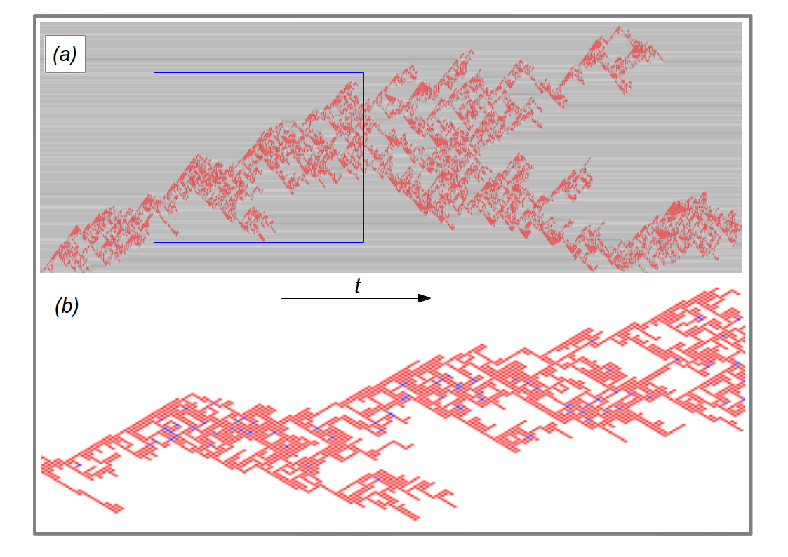
Figure 1: (Color online) A typical avalanche of boundary driven Oslo model (time flows towards right). (a) The stress profile: $z_{i}\leq 2$ are marked as gray (different shades) and sites with $z_{i}>2$ are marked as red. (b) A portion of the avalanche, marked as a rectangle in (a), is zoomed to view single (red) and multiple (blue) topplings.

In the original version, the model is driven by adding grains of rice at the left boundary. In terms of stresses this means that the system is driven by increasing $z_{1}$ by one unit. If this leads to an instability, the entire avalanche of topplings is done before $z_{1}$ is increased again. A typical avalanche in the boundary driven case, starting from a single seed is shown in Fig. 1.

We say that the pile is bulk-driven, when we choose a random site $i\in]1,L[$ and increase its stress by 1 unit. Notice that this would be a somewhat unusual drive in a real rice pile: It would correspond to adding 1 rice grain at sites $1,2,\ldots i$ each. We expect that avalanche size distributions for bulk-driving will be different from those for the boundary-driven case, but some critical exponents like $D$ and $z$ (defined below) would be the same.

In addition, we expect that finite size corrections will be very different. For boundary driving, the only large length scale is the distance $L$ to the far boundary. For bulk driving, another length scale comes into play: the (random) distance of point of addition from the boundary. This is, of course, averaged over, but typically gives rise to much larger finite size corrections.

II.3 Fixed energy version

Finally, we shall also consider the FES version with periodic boundary conditions. In that case no stress can get lost. If we drive the system by adding stress, we sooner or later must reach the critical point where avalanches never stop. On the one hand, this is the cleanest case because finite size corrections are minimal. On the other hand, as pointed out in the introduction, simulations at the critical point are not trivial in this version.

In the subcritical case simulations are rather straightforward: starting with any initial configuration with $\langle z\rangle=Z/L<z_{c}$, we follow the avalanche (if at least one site is unstable) until it dies. After that, all sites are stable. If $\langle z\rangle$ is sufficiently close to $z_{c}$, there will be some sites with $z_{i}=2$. We now trigger a new avalanche by declaring one (or several) of these sites as unstable (if no site with $z_{i}=2$ exists, we increase $Z$, until we are close enough to the critical point).

Notice that declaring a stable site with $z_{i}=2$ does not alter the NCS, hence we do not expect to encounter the problems mentioned in footnote3 .

Simulations are equally straightforward in the supercritical case, where the above procedure soon leads to an infinite avalanche. As in the BTW case Fey1 , an avalanche will not stop after each site has toppled once, and this will happen in general after $\ll O(L)$ time steps.

On the other hand, following avalanches on large lattices until they die is not a viable option at the critical point, because avalanches may not die even after very many time steps. In that case we have (at least) three options how to proceed:

(a) We could use finite lattices and perform a finite size scaling (FSS) analysis Christ:2004 . This gives reasonable results, although it requires more numerical effort and the extrapolation $L\to\infty$ is associated with the usual uncertainties of any extrapolation.

(b) We could introduce a small amount of dissipation (i.e., with some very small probability $\epsilon$, Eq. (2) is modified such that one of the neighbors has its stress not increased), and extrapolate to $\epsilon\to 0$. This was the strategy used in Mohanty:2002 ; Mohanty:2007 . While this should give cleanest results, it has the drawback that it requires more simulations and also involves an extrapolation. We did not try it in the present work.

(c) We could simply cut the evolution at some large time $T_{\rm max}$. This seems to be the strategy chosen in most previous simulations (e.g. in the BTW simulations of Vesp:2000 ). As we shall see, results can be extremely misleading, unless this is done carefully.

II.4 Initial conditions

We know from previous simulations and from test runs that $z_{c}\approx 1.7326$. We now pick a rational number $n/m$ slightly smaller than $z_{c}$, e.g. $n/m=45/26=1.7307\ldots$. A sequence $w_{m,n}$ of $m$ digits $z_{i}\in\{1,2\}$ is then constructed such that $\sum_{i}z_{i}=n$ and that $w_{m,n}$ is as uniform as possible. For $(n,m)=(45,26)$ such a sequence is $w_{26,45}=(12^{2}12^{3}12^{3}12^{3}12^{2}12^{3}12^{3})$ or any of its cyclic permutations. The initial configuration is then simply a repetition of $L/m$ such words, provided $L$ is a multiple of $m$. In practice, we used rational approximants closer to $z_{c}$, such as 149/86 or 473/273.

II.5 Transients

First we discuss transients in the boundary-driven case. To see most clearly the transients, we used very large lattices ($\geq 10^{7}$ sites) driven at the left boundary. We call the “active region” at time $t$ the part $[1,i_{\rm max}(t)]$, where $i_{\rm max}(t)$ is the rightmost point that had toppled at some time $t^{\prime}\leq t$. We monitor the evolution while $i_{\rm max}(t)<L$, i.e., while the active region still spreads. In Fig. 2 we show the total number of topplings, starting from the initial time $t=0$ till the time the disturbances from the boundary first reach the site $i=i_{\rm max},$ for different initial configurations. Notice that this gives a lower estimate for the transient CPU time, because even if the active region covers the entire lattice, it is still not clear whether it has the correct NCS correlations. The top five curves are for random 1 / 2 sequences. If $z_{0}=\langle z_{i,0}\rangle\ll z_{c}$, clearly $s\sim i_{\rm max}^{3}$. As $z_{0}$ comes closer to $z_{c}\approx 1.73260$, this increase is slower, but it is still much faster than the increase $s\sim i_{\rm max}^{2}$ observed for periodic initial configurations.

Figure 2: (Color online) Number of topplings on a semi-infinite lattice driven at its left end, until a site at distance $i_{\rm max}$ from this end is first toppled. Each curve is based on $\approx 1000$ runs.

While Fig. 2 suggests that periodic initial configurations lead to much shorter transients, it could still be that the configurations at the time when $i_{\rm max}$ is reached have much larger fluctuations and densities far from the asymptotic one. That this is not true, and that periodic initial configurations lead both to much smaller fluctuations and to correct densities is seem from Fig. 3. There we plot the average density $\langle z\rangle_{\rm active}$ in the active region, obtained in one single run, against an inverse power of $i_{\rm max}$. The lowest five curves in this plot correspond all to periodic initial configurations, with increasing values of $z_{0}$. They show that both deviations from the asymptotic density and fluctuations become smaller as the initial density approaches the stationary one. On the other hand, starting with a random configuration leads to huge fluctuations, even if its density is close to the stationary one.

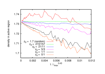
Figure 3: (Color online) Average density in the active region, plotted against an inverse power of the size $i_{\rm max}$ of the active region, for different initial configurations. Each curve is based on a single run. For all curves the stationary density is reached as $i_{\rm max}\to\infty$, but the speed of convergence and the fluctuations depend strongly on the choice of initial state. Periodic initial states with density close to the stationary one are optimal. Notice that what looks like a horizontal straight line is indeed the data for $z_{0}=272/157=1.732484$.

III Determination of critical exponents from numerical simulations

In subsections A to C we shall mostly discuss simulations with open boundaries, which are driven by adding stress at the left boundary (with the exception of Figs. 2 to 6, which are indeed identical for open systems driven in the bulk). The fixed-energy version is discussed in subsection D, while properties of avalanches in bulk-driven open systems are treated in subsection E.

III.1 The stationary state and hyperuniformity

We will now discuss the various observables measured in our simulations, and their analysis in terms of the finite-size scaling theory. The critical exponent $\nu$ is defined in terms of the dependence of the correlation length $\xi$ on the distance from the critical point $\epsilon=\rho-\rho^{*}$, where $\rho^{*}$ is the critical density, by the relation

$$\xi\sim\epsilon^{-\nu}.$$ (3)

According to the finite-size scaling theory (FSS), a system with finite size $L$ at criticality will behave like an infinite system with finite correlation length $L$. Thus, we expect

$$\langle z\rangle_{L}-z_{c}\sim L^{-1/\nu}$$ (4)

The dependence of $\langle z\rangle_{L}$ on $L$ provides a straightforward direct determination of $\nu$. In Fig. 4 we show how the average stress $\langle z\rangle=L^{-1}\sum_{i=1}^{L}z_{i}$ depends on $L$. In the main plot we show the raw data, and in the inset a plot which suggests the precise finite size corrections. Indeed, for reasons that will become clear in a moment, we used in Fig. 4 not only data obtained on boundary driven systems, but we averaged also over systems driven in the bulk, both at random sites and also just at the center site. The result of Fig. 4 can be summarized as

$$\langle z\rangle=z_{c}+c/L^{\sigma}$$ (5)

with

$$z_{c}=1.732594(4)\;,\quad\sigma=1/\nu=\;\;0.74(1),$$ (6)

while the precise value of $c$ depends strongly on $\sigma$. The best previous estimates of $z_{c}$ were $1.7326(3)$ for boundary driven and $1.734(2)$ for bulk driven open systems, and $1.73260(2)$ for the FES version Christ:2004 . We are not aware of a previous estimate of $\sigma$.

Another way to determine $\nu$ is to look at the effects of the boundary on the density profile. Let $\rho(i)$ be the mean density of particles at site $i$ in the steady state of the driven sandpile. From the abelian property one obtains the following result : $\rho(i)$ is independent of the way the pile is driven.

Proof: Let $a_{i}$ be the operator corresponding to adding a particle at $i$ and letting a subsequent avalanche evolve until a stable state is reached again. Let $|\Phi\rangle$ be the statistically stationary (macro-)state obtained by driving at site $i$ with probability $p_{i}$. It satisfies $|\Phi\rangle=W|\Phi\rangle$ with $W=\sum_{i}p_{i}a_{i}$ . Since all $a_{i}$ commute due to the abelian property, they can be diagonalized simultaneously, and $|\Phi\rangle$ is an eigenvector of each $a_{i}$ with eigenvalue $1$, and if the Markov process can reach all recurrent states, it is the only eigenvector with this property, and so independent of the distribution $\{p_{i}\}$.

We have checked this directly in simulations. In Fig. 5, we plot $\rho(i|j_{0})$ the average stress at $i$ when the system is driven at site $j_{0}$. In the main plot of Fig. 5 we show differences between averages measured at the same $i$ but for different $j_{0}$. These data are for a very small system, but the same was found also for larger $L$. This is true also for random bulk driving, as we indeed verified numerically.

From scaling theory, we expect $\rho_{i}$ to differ from $z_{c}$ as

$$\rho(i)-z_{c}\sim i^{-1/\nu}.$$ (7)

We show the variation of $\rho_{i}$ with $i$ in Fig. 6.

The stress density, averaged over a finite block of size $k$, will in the critical state show fluctuations of order $k^{-1/\nu}$, hence the total stress $Z$ in this block will fluctuate by a typical amount $k\times k^{-1/\nu}$. This gives

$${\rm Var}[Z]\sim L^{\zeta}=L^{2(1-1/\nu)}$$ (8)

giving the hyperuniformity exponent $\zeta=2(1-1/\nu)$. The variation of ${\rm Var}[Z]$ with $k$ is plotted in Fig. 7. We see that the value of $\zeta=1/2$ fits the data very well. Based on the results presented, we conjecture that $\nu$ is exactly equal to the simple fraction $4/3$.

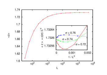
Figure 4: Average stress $\langle z\rangle$ of driven systems with open boundaries as a function of $L$. Main: log-linear plot of the raw data. Inset: The same data plotted such that one can determine more precisely the finite size corrections. More precisely, on the $x$-axis is plotted $L^{-\sigma}$ with $\sigma$ either 0.76, 0.74, or 0.72. If $\sigma$ were equal to the exponent of the leading finite size correction, then the plot of $\langle z\rangle$ versus $L^{-\sigma}$ would be asymptotically a straight line. Since finite size corrections are very large, data would be indistinguishable from straight lines in such a plot for a wide range of $\sigma$. Therefore we add to $\langle z\rangle$ a term linear in $L^{-\sigma}$, such that the curves become roughly flat near the origin. The curve which is most straight at the origin gives then the true correction to scaling exponent.

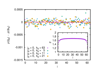
Figure 5: (Color online) The inset shows the stationary profile $\rho(i)$ for $L=64$. To verify that it is indeed left-right symmetric, we show in the main plot differences between values of $\rho(i)$ measured at the same site $i$, but for runs where the system was driven at different values $j_{0}$ resp. $k_{0}$. The estimated statistical error for these differences was between $\pm 0.0001$ and $\pm 0.0002$.

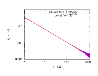
Figure 6: (Color online) Log-log plot of stress depletion near the end points versus distance from the end (more precisely from the point $x=1/2$, half way between the site $i=0$ where $\rho(i)$ is zero, and the site $i=1$ where it first becomes positive). Lattices ($L\geq 2^{15}$) are sufficiently large so that finite size corrections should be negligible.

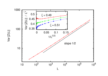
Figure 7: (Color online) The main plot shows a log-log plot of ${\rm Var}[Z]$ versus $L$, together with a straight line that suggests ${\rm Var}[Z]\sim L^{1/2}$ with visible corrections. The inset suggests that these corrections decrease roughly as $L^{-1/2}$.

III.2 Avalanche size distributions

For the distribution of avalanches, our clearest data come from the boundary-driven case where one adds stress at the left boundary, and lets it dissipate through the right one.

Let us first discuss the avalanche size distribution $P(s,L)$, where $s$ is the number of topplings in an avalanche. We expect the scaling law

$$P(s,L)=s^{-\tau}f(s/\varphi(L))\times[1+\frac{a}{L^{x}}+\ldots],$$ (9)

with

$$\varphi(L)=L^{D}\times[1+\frac{b}{L^{\omega}}+\ldots],$$ (10)

where the last factors in both expressions correspond to finite size corrections.

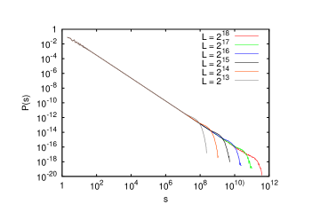
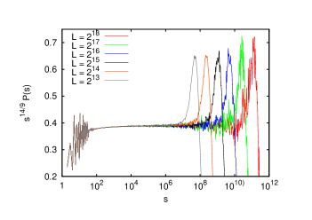
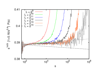
Figure 8: (Color online) Avalanche size distributions for the open systems driven at the left boundary. Panel (a) shows the raw data (for the largest lattices sizes only, to avoid overcrowding). Panel (b) shows the same data multiplied by $s^{14/9}$. If this exponent is equal to $\tau$, the central parts of the curves should be flat. In view of the substantial corrections to this, we plotted in panel (c) the data (for smaller $L$, since they have less statistical fluctuations) multiplied by a further factor $(1+a/s^{x})$, with $x=0.4$. The two straight lines in panel (c) indicate the error margins $\pm 0.0005$ of $\tau$. The numbers of avalanches used for these figures range between $>2\times 10^{10}$ for $L\leq 4096$, $1.7\times 10^{9}$ for $L=131072$, and $3.5\times 10^{9}$ for $L=262144$. The fluctuations seen for $s<100$ are not statistical, but are systematic, and are related to the structure of the state-space of recurrent stable configurations Chua-Christ .

In Fig. 8 we show $P(s,L)$ for values of $L$ between 512 and $2^{18}$. The raw data shown in panel (a) just demonstrate the impressive range, but they are not really informative. Multiplying the data with $s^{\tau}$ as in panel (b) shows already much more details. But it still does not allow to make a precise estimate of $\tau$. For this we have to include finite size corrections, as in panel (c) (where we mostly plotted data for the smallest values of $L$, which were not shown in panels (a) and (b)). The correction to scaling exponent is close to 1/2, and we will justify the choice $0.4$ below. Our best estimate of $\tau$ is $1.5556\pm 0.0005$. This is a factor 4 more precise than the best previous estimates $1.556\pm 0.002$ Christ:96 ; Pruss:2003 ; Paczuski . It strongly suggests that $\tau=14/9$ exactly, as conjectured in Christ:2004a (a ten times more precise value was claimed in Christ:2004a , but this was revised in a later paper by the same author Christ:2004 ).

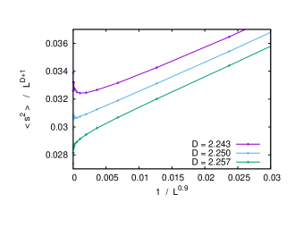
Figure 9: (Color online) Re-scaled second moments of avalanche sizes for the boundary model, plotted against $1/L^{0.9}$. The moments are divided by powers of $L$, such that the curve would be straight if the power were equal to $D+1$ and the correction to scaling exponent were $\omega=0.9$. This is indeed the case for $D=9/4$. The other two curves (with exponents $9/4\pm 0.007$) are clearly sub- and supercritical.

Using Eqs. (9), (10), and the fact that $\langle s\rangle=L$ (which is true exactly, without any finite size corrections) gives

$$D=(2-\tau)^{-1}=9/4\pm 0.002\quad{\rm and}\quad\omega=xD\approx 0.9.$$ (11)

Superimposing the peaks in Fig. 8b would give a compatible but much less precise estimate of $D$ because of the finite size corrections in $\varphi(L)$. But a more precise value, with error bars similar as those that follow from the scaling relation, can be obtained from higher moments of $s$. From Eq. (9) we expect

$$\langle s^{k}\rangle\sim L^{(k+1-\tau)D}=L^{D+1}\times[1+\frac{b^{\prime}}{L^{\omega}}].$$ (12)

In Fig. 9 we plot $L^{y}\langle s^{2}\rangle$ against $1/L^{0.9}$ for three values of $y$. The central curve is for $y=13/4$, and it is a perfect straight line up to fluctuations for the two largest lattices ($L=2^{18}$ and $L=2^{19}$). On the other hand, the two other curves are clearly sub- and supercritical. A similar result is obtained from the third moment (not shown). Apart from verifying the estimate of $D$, these data suggest very strongly that indeed the correction to scaling exponent is $\omega=0.9$.

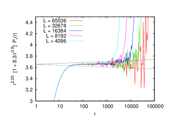
Figure 10: (Color online) (a) Log-log plot of $P_{r}(r,L)$, the spatial size distribution of avalanches for boundary driven systems, multiplied by $r^{9/4}$. (b) The same data, but multiplied by $1+8.3/r^{0.9}$ and plotted on a log-linear plot. The straight lines indicate the estimated errors $\pm 0.002$

The distribution of spatial extensions of avalanches, $P_{r}(r,L)$, we assume the scaling form

$$P_{r}(r,L)\approx r^{-\tau_{r}}g(r/L),$$ (13)

As we have $s\sim R^{D}$, it is easily seen that $\tau_{r}=1+(\tau-1)D$. For $D=9/4$, and $\tau=14/9$, we get $\tau_{r}=9/4$.

Plots analogous to Fig. 8b and 8c are shown in Fig. 10. This time the corrections to scaling are much bigger, but they seem to be described again to leading order by a rational power. The value $\tau_{r}=9/4$ fits our data well, with an error of $\pm 0.002$. At the same time, accepting the scaling $s\sim r^{D}$ in the scaling region, we predict the correction to scaling exponent as $0.4\times 9/4=0.9$, in perfect agreement with the data.

III.3 Temporal evolution of avalanches

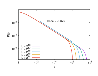
Figure 11: (Color online) Log-log plot of $P_{t}(t,L)$ (panel a), $N(t,L)$ (panel b), and $R(t,L)$ (panel c). In each plot, only data for $L\geq 16384$ are shown. The straight lines indicate power laws in the central (scaling) region.

We now discuss the time-dependent exponents of the avalanches. We define the dynamical exponent $z$ by the relation

$$R(t)\sim t^{1/z}$$ (14)

where $R(t)$ is the average distance of topplings at time $t$ from the boundary where the avalanches were triggered. Other related quantities are $P_{t}(t)$ and $N(t)$, which are respectively the probability that the avalanche survives up to time $t$, and the average number of topplings at time $t$ in the avalanches that survive up to time $t$. We define the exponents $\eta$ and $\delta$ by the relations

$$P_{t}(t)\sim t^{-\delta}\quad{\rm and}\quad N(t)\sim t^{\eta}.$$ (15)

Results of these measurements are shown in Fig. 11. They all show very clean scaling regions, with

$$\delta=7/8,\quad\eta=-3/10,\quad{\rm and}\quad z=10/7.$$ (16)

We do not quote formal error bars, because by now we obviously conjecture that these rational numbers are exact, and any error estimate (which by its very nature is subjective, critical exponents being obtained by extrapolating data) would probably be biased by this conjecture. We nevertheless can say informally that plots analogous to Figs. 8c and 10b suggest $\delta=0.875(1),\eta=-0.300(1)$, and $1/z=0.700(2)$.

Typical previous estimates were $\delta=0.85(2)$, $\eta=0.33(2)$, and $z=1.42(2)$ Bona-thesis . They were, however, made by assuming a Manna universality class and thus lumping together simulation results from various models. As a rule of thumb, our present estimates are an order of magnitude more precise than previous ones. On the other hand, extracting correction to scaling exponents from Fig. 11 was not very successful, because obviously more than one correction term is important in each case. Presumably, there are also important analytic corrections resulting from an inherent uncertainty how to define $t$ up to an arbitrary constant of order 1.

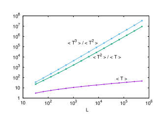
Figure 12: (Color online) Log-log plots of the average lifetime $\langle T\rangle$ of boundary-driven avalanches, and of moment ratios $\langle T^{k+1}\rangle/\langle T^{k}\rangle$ for $k=1$ and $k=2$.

Another estimate of $z$ can be obtained from the moments of $T$, the life time of avalanches. When defining $\langle T^{k}\rangle$, one has to specify how avalanches with different size $s$ are weighted. In Fig. 12 we show results for $\langle T\rangle,\langle T^{2}\rangle/\langle T\rangle$, and $\langle T^{3}\rangle/\langle T^{2}\rangle$, where $T=s^{-1}\sum_{{\rm topplings}j}t_{j}$ and $t_{j}$ is the time of the $j$-th toppling in the parallel update scheme. We see no clear scaling law for $\langle T\rangle$, a scaling law with large finite size corrections for $\langle T^{2}\rangle/\langle T\rangle$, and finally a clean scaling with reasonably small finite size corrections for $\langle T^{3}\rangle/\langle T^{2}\rangle$,

$$\langle T^{3}\rangle/\langle T^{2}\rangle\sim L^{1.43(1)}.$$ (17)

The latter is consistent with our conjectured exact value $z=10/7$.

III.4 The Fixed-energy sandpile: closed boundaries case

III.4.1 Supercritical systems: The order parameter exponent

As we said in the introduction, simulating the fixed “energy” (i.e. stress) model is easiest and most straightforward away from the critical point. In contrast, measuring the properties of single avalanches is non-trivial both in the critical and in the supercritical phase. But estimating the density $\rho_{a,\infty}$ of active sites in a stationary supercritical state, and thus the order parameter $\beta$ defined through

$$\rho_{a,\infty}\equiv\lim_{t\to\infty}\rho_{a}(t)\sim(\langle z\rangle-z_{c})^{\beta},$$ (18)

is easy. We start with a periodic configuration with the desired total stress (which implies also that we use for $L$ a multiple of the period). There will be $O(L)$ sites with $z_{i}=2$, half of which are declared as unstable. We then follow the evolution until stationarity of $\rho_{a}$ is reached and enough statistics is collected thereafter.

Figure 13: (Color online) Log-log plot of $\rho_{a,\infty}$ against $\langle z\rangle-z_{c}$. The straight line indicates the power law predicted by the scaling theory. The best fit would indeed be obtained with an exponent $0.243(5)$. The leftmost point was obtained by simulating 40 lattices with $L=10^{6}$ for $5\times 10^{7}$ time steps.

The approach to stationarity will be roughly exponential in the far supercritical regime, but in the critical region it will follow a power law. In the latter region the difference between the periodic initial state and the true NCS will become important, and we shall defer the discussion of this subtle case to a later subsection. Here it is sufficient to point out that in the worst case (i.e. closest to the critical point, where the correlation length becomes comparable to $L$) the transient time increases as $L^{z}$. As we have seen, the correlation length scales as $\xi\sim(\langle z\rangle-z_{c})^{-\nu}$ with $\nu=4/3$. Thus we can use lattices of sizes up to $L\approx 10^{6}$, simulated over $5\times\approx 10^{7}$ time steps, to test Eq. (18) down to $\langle z\rangle-z_{c}\approx 0.00005$.

Fig. 13 shows results from such runs. Each point in this plot is obtained from at least 40 such runs, and it was verified that the density of activity had become stationary. The straight line indicates the exponent

$$\beta=5/21$$ (19)

that follows from the scaling theory discussed below. The data shown in the figure would by themselves give a best fit $\beta=0.243(5)$, compatible with the above.

To obtain Eq. (19), we notice first that FSS suggests that for finite $L$ and exactly at criticality $\rho_{a,L}\sim L^{-\beta/\nu}$. The number of topplings in large avalanches (those which dominate the higher moments of $s$) scales then as $L$ times this density times the duration of the avalanches,

$$s\sim L\times L^{-\beta/\nu}\times L^{z}.$$ (20)

Assuming that $s\sim L^{D}$ with $D=9/4$ gives then

$$\beta=(1+z-D)\nu=5/21.$$ (21)

Table 1: Estimates of the critical exponent $\beta$ defined in Eq. (18). The acronyms for the various models are explained in the references.

0.24(3)	Bona-thesis	overall Manna class
0.42(2)	Dick:2001	Manna
0.416(4)	Dickman-Tome	restricted Manna
0.41(1)	Dick:2002	restricted Manna
0.289(12)	Dick:2006	restricted Manna
0.29(2)	Kockel	CDP
0.28(2)	Ramasco	CDP
0.382(19)	Lubeck:2004	DCMM
0.277(18)	BBBMH	CCMM
0.308(2)	BBBMH	CTTP
0.275(6)	BBBMH	CLG
0.277(3)	Fiore	modified CLG
0.25(3)	Lesch	qEW
0.33(2)	Duemmer	qEW
0.250(3)	Kim-Choi ,Song-Kim	qEW
0.245(6)	Ferrero	qEW
0.396(5)	Lee	Oslo
0.243(5)	present work	Oslo, direct fit
5/21 = 0.2380…	present work	Oslo, scaling relation
0.2764…	Hinrichsen	DP

There exist a large number of previous estimates of $\beta$, either for the Oslo model itself or for other models which are supposed in the same (Manna) universality class, see Table 1. They are all are much bigger, with one notable exception: $\beta=0.24(3)$ was obtained in Bona-thesis . All other estimates are supposedly more precise but outside our error bars. The problem in determining $\beta$ is obviously the large corrections to scaling which are seen in Fig. 13, and which require very large systems to be studied. In Table 1 we quote also the value for DP. In many previous papers it was concluded that the Manna class has to be distinct from DP, mainly because it has a larger value of $\beta$. We see now that the opposite is true, and Manna $\neq$ DP because its $\beta$ is smaller than that of DP.

We include in Table 1 also three estimates for the qEW model. Since the mapping of the Oslo model onto interface pinning is such that the interface height is just the number of topplings, the activity density $\rho_{a}(t)$ is just the average speed of the interface at time $t$. The value quoted in Table 1 is for the exponent (called $\theta$ in Kim-Choi ; Song-Kim ) that described how the speed increases in the de-pinned phase with the distance from the critical point, $v\sim(F-F_{c})^{\theta}$.

In Corral , the relation between

$$\beta=(1+z-D)/(3-D)$$ (22)

was proposed. Although the numerical value of $\beta$ obtained thereby in Corral is different from ours, Eq. (22) is satisfied by our exponents. Together with Eq. (19) it gives

$$\nu=1/(3-D).$$ (23)

Finally, we note that for FES with deterministic toppling rules, it has been noted that the critical density at which infinite avalanches first appear, depends on the starting configuration Fey1 . For sandpiles with stochastic toppling rules, this is not a problem, and the SOC and FES versions of the Oslo model have the same critical density.

III.4.2 Subcritical single-seed avalanches

The next easy case are isolated avalanches in the subcritical phase. We again start with a periodic configuration (this time with $\langle z\rangle<z_{c}$). We declare all sites (including those with $z_{i}=2$) as stable. To trigger an avalanche we simply pick a random site among those with $z_{i}=2$ and declare it as unstable. This avalanche will be finite with probability 1 and will have also finite size, thus we can follow its evolution until it dies and the configuration is stable again. After that, we again declare a random site with $z_{i}=2$ as unstable and repeat.

By measuring avalanche sizes, we verified that transients are very short: Average avalanche sizes converge within error bars to a stationary value, after each site has toppled less than 1000 times, even when $\langle z\rangle$ is very close to $z_{c}$. Thus we can again get good statistics for lattices with $L$ up to $10^{6}$. Lattices of this size are indeed needed in order to avoid finite size effects, if we want to measure very close to the critical point.

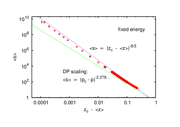
Figure 14: (Color online) Log-log plot of $\langle s\rangle$ against $z_{c}-\langle z\rangle$ for subcritical avalanches in the FES version. The upper straight line indicates the power law predicted by the scaling theory. The best fit would indeed be obtained with an exponent $2.68(2)$. The lower straight line shows the behavior that would have been expected, if the Oslo model were in the DP universality class. The leftmost point was obtained by simulating 3600 avalanches on a lattice with $L=5\times 10^{5}$.

Results are shown in Fig. 14, where we plot $\langle s\rangle$ against the distance from the critical point. We see a clear power law in the critical region, but important scaling corrections when $z_{c}-\langle z\rangle$ becomes large. The latter could have suggested that the power is the same as for DP, but this is actually excluded: While the DP exponent $\gamma$, defined as

$$\langle s\rangle\sim(z_{c}-\langle z\rangle)^{-\gamma},$$ (24)

is 2.278 Hinrichsen , a direct fit to our data would give $\gamma=2.68(2)$. The upper straight line shown in Fig. 14 represents our scaling conjecture

$$\gamma=2\nu=\;\;8/3,$$ (25)

which follows from $\langle s\rangle\sim L^{2}$ via FSS and which is fully compatible with the directly measured value.

III.4.3 Finite-size scaling: Critical avalanches on finite lattices

Exactly at the critical point, we cannot use either of the two strategies discussed in the previous subsections. In this subsection we simulate single avalanches, triggered in the way described above, on lattices of sufficiently small $L$ so that we can follow all of them until they die. Avalanche distributions will be discussed below, but first we shall discuss moments of their sizes and durations.

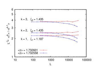
Figure 15: (Color online) Panel (a): Log-log plot of $\langle s\rangle$ (lowest triple of curves) and $\langle s^{k}\rangle/\langle s^{k-1}\rangle$ for $k=2$ and 3 (topmost triples) against $L$. Each curve in each triple corresponds to a different periodic start configuration (periods 101, 273, and 86 from top to bottom), and each value of $L$ is a multiple of the corresponding period. The data are divided by $L^{2}$ which makes the central curve in the lowest triple horizontal and makes the central curves in the two upper triples scale as $L^{1/4}$ (straight line). Panel (b): Analogous results size-weighted for moments of avalanche life times. This time only data for the two smaller values of $\langle z\rangle$ are shown, and all data are divided by powers of $L$ which make the critical curve of each pair horizontal.

Moments of the avalanche size $s$ are shown in Fig. 15a, while moments of their life times are shown in panel (b). The latter were computed as in subsection III.3. In panel (a) we show results for three values of $\langle z\rangle$ close to $z_{c}$, while results for only two of them are shown in panel (b).

The bottom triple of curves in panel (a) show $\langle s\rangle/L^{2}$. These values are independent of $L$ within errors for the central curve which is essentially critical, showing that

$$\langle s\rangle\sim L^{2}$$ (26)

for critical avalanches in the FES ensemble, just as it is for bulk driven avalanches on open lattices. This is not entirely trivial, since the argument predicting this scaling for open systems no longer holds. The fact that we nevertheless find the same scaling in both ensembles is a strong indication that the avalanches have the same statistical properties.

The same conclusion is reached by looking at the two upper triples of curves in panel (a) which show the ratios $L^{-2}\langle s^{k}\rangle/\langle s^{k-1}\rangle$ for $k=2$ and 3. Here the critical curves show that all moments satisfy exactly the same critical scaling $\langle s^{k}\rangle\sim L^{2+9k/4}$ as for open systems.

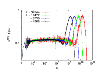
Figure 16: (Color online) Log-log plot of the avalanche size distributions for the fixed-energy version at $\langle z\rangle=1.732601$, and for different lattice sizes which are all multiples of 273. The actually plotted data are $s^{10/9}P(s)$.

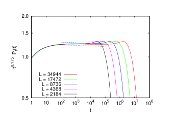
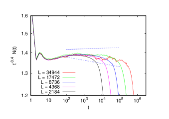
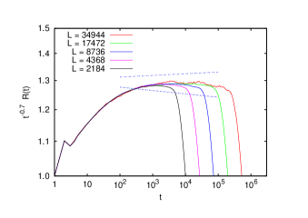
Figure 17: (Color online) Log-log plots of $P_{t}(t,L)$ (panel a), $N(t,L)$ (panel b), and $R(t,L)$ (panel c). In each plot, the raw data were divided by the conjectured power laws, i.e. the actually plotted data are $t^{3/8}P_{t}(t,L),t^{-2/5}N(t)$, and $t^{-7/10}R(t)$. As in Fig. 16, $R(t)$ is the rms. distance from the first toppling. In each panel, the straight lines indicate the error bars mentioned in the text.

The data for avalanche durations shown in panel (b) tell a similar story. The two topmost pairs of curves show that $\langle T^{k}\rangle/\langle T^{k-1}\rangle$ with $k\geq 2$ scale with the same power of $L$, which is within errors the same as the exponent $z$ found also in the open case (the fitted value of $z$ now is 1.438(10), while our previous estimate was $10/7=1.4286$). In agreement with the bulk-driven open case, $\langle T\rangle$ now also shows good scaling, with exponent $1.187(10)$.

Distributions of avalanche sizes and of the three time dependent properties $P_{t}(t),N(t)$, and $R(t)$ are shown in the Fig. 17 (we did these simulations at $\langle z\rangle=1.732601$ before arriving at the final estimate for $z_{c}$ in Eq. (6), but the small deviation from the best estimate of $z_{c}$ should not matter much). For $P(s)$ we show only a plot analogous to Figs. 8b and 23, where we divided the raw data by the supposed power law $s^{-\tau_{\rm bulk}}$, see Fig. 16. Although the scaling is not perfect, the improvement compared to the bulk driven case with open boundaries shown in Fig. 23 is dramatic. Now we can argue rather convincingly that $\tau_{\rm bulk}=10/9$. The best estimate based on this plot alone would be $\tau_{\rm bulk}=1.10(1)$, based both on the scaling region and on the heights of the peaks (which should also scale as $s^{-\tau_{\rm bulk}}$).

The three panels of Fig. 17 show $t^{3/8}P_{t}(t),t^{-2/5}N(t)$, and $t^{7/10}R(t)$. The actual best exponent estimates based on these plots alone would be $\delta_{\rm bulk}=0.175(3),\eta_{\rm bulk}=0.398(3)$, and $z_{\rm bulk}=0.699(3)$, as indicated by the dashed straight lines in each panel.

Within the statistical errors, the sum $\delta+\eta$ is the same as for open boundary driven systems,

$$\delta_{\rm bulk}+\eta_{\rm bulk}=\delta+\eta=23/40.$$ (27)

This means that the activity $N(t)/P_{t}(t)$ per surviving avalanche shows the same scaling in both cases. It should indeed scale as the product of the activity density in the active region (which scales as $t^{-\beta/z/\nu}$, as we shall see later) times its spatial extent (which scales as $t^{1/z}$). Therefore

$$\delta+\eta=(1-\beta/\nu)/z$$ (28)

III.4.4 Simulations involving termination of the evolution in non-stationary states

So far we have only discussed simulations of the fixed-energy Oslo model where it was either not necessary to terminate the evolution because avalanches died anyhow, or where the system had already reached a stationary state. For simulating systems very close to the critical point, it seems however necessary to terminate the evolution before avalanched have died or before stationarity is reached. As we shall see, extreme case is needed in interpreting such simulations.

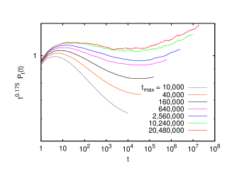
Figure 18: (Color online) Log-log plots of rescaled survival probabilities $t^{3/8}P_{t}(t)$, if the evolution of each still surviving avalanche is terminated at time $t_{\rm max}$. Here the largest lattices (for the largest $t_{\rm max}$) had $L=2^{21}$. The average stress was $1.732591$ (i.e., slightly subcritical), but it was verified that results were indistinguishable at slightly supercritical $\langle z\rangle$. From our previous simulations we would have expected the curves to become horizontal for large $t$ and large $t_{\rm max}$.

Let us first discuss simulations of single avalanches, triggered by declaring random sites with $z_{i}=2$ in an otherwise stable configuration as unstable. If an avalanche survives for a time $>t_{\rm max}$, its evolution is cut off by declaring all sites with $z_{i}=2$ as stable. Since only very few avalanches survive until $t_{\rm max}\gg 1$, one might hope that this gives reasonable results if $t_{\rm max}$ is sufficiently large. Indeed, this strategy is rather common in studies of FES sandpile models. Fig. 18 shows survival probabilities $P_{t}(t)$ on very large lattices and at $\langle z\rangle$ very close to criticality, for different values of the cutoff $t_{\rm max}$, ranging from $10^{4}$ to $2\times 10^{7}$. Since we have multiplied the data by the factor $t^{\delta}$, we should have expected the curves to become horizontal for large $t$ and large $t_{\rm max}$. They do indeed become horizontal for $1\ll t\ll t_{\rm max}$, but estimating $\delta$ from the data with largest $t$ would give gross inconsistencies. The same is true for $N(t),R(t)$, and $P(s)$. In all these cases we could get consistent results by first taking $t_{\rm max}\to\infty$ and only then going to large $t$, but this would not be very practical.

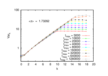
Figure 19: (Color online) Log-log plot of variances of the total stress on intervals of length $2^{k}$, ${\rm Var}_{k}={\rm Var}[Z_{k}]$ with $Z_{k}=\sum_{i=i_{0}}^{i_{0}+k-1{\rm mod}L}z_{i}$. Each curve was obtained by terminating the evolution of avalanches at $t_{\rm max}$, and the total CPU time used for each curve was roughly the same. Lattice sizes were up to $4\times 10^{6}$, and $\langle z\rangle$ is very close to critical.

The reason for this failure is that if avalanche evolution is stopped at $t_{\rm max}$, also the correlations in the NCS needed to make it critical and hyperuniform cannot develop at distances $>t_{\rm max}^{1/z}$. Essentially, criticality and hyperuniformity are then confined to scales $<t_{\rm max}^{1/z}$ and correlations at larger scales are those of the initial state and different from those in the NCS, even if the simulation is kept going for extremely long times, see Fig. 19. Since total CPU time was roughly the same for each curve in Fig. 19, it seems unlikely that longer runs would establish critical correlations on substantially larger scales.

Thus simulations of single avalanches where the evolution is stopped at finite times seem not very useful. But simulations near criticality where a finite fraction (50%, say) of sites with $z_{i}=2$ are initially unstable are useful, and are crucial for understanding scaling. Let us denote by $\epsilon=\langle z\rangle-z_{c}$ the distance from the critical point. Naively, one should expect that activity satisfies in this case a finite size scaling (FSS) ansatz

$$\rho_{a}(t,L,\epsilon)\sim t^{-\theta}F(\epsilon L^{1/\nu},\epsilon t^{1/\nu_{t}})$$ (29)

with $\nu_{t}=z\nu$. In order to agree with Eq. (18), the scaling function $F(x,y)$ has to scale for $y\to 0$ and $x\to\infty$ as $y^{\beta}$ and furthermore $\theta=\beta/\nu_{t}$. The problem is of course that we expect this to hold when the state at $t=0$ is a NCS, but we have no foolproof way to construct one. Even worse, a NCS would have no unstable sites. In studying single avalanches, it seems reasonable that declaring a single $z_{i}=2$ site as unstable should be a negligible perturbation, but now we want to make a finite fraction unstable. It is far from obvious what effect this has, but we can turn to simulations to find out numerically.

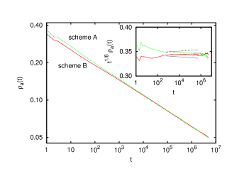
Figure 20: (Color online) Main plot: Log-log plot of $\rho_{a}(t)$ for $\langle z\rangle=359/208=1.732596$ and $L=524140$. For the upper curve (scheme A) each run started from an periodic configuration, while the lower curve (scheme B) used for each run the final state of the previous run, with half of the sites with $z_{i}=2$ declared as unstable. Each curve is based on 508 runs. The inset shows the same data multiplied by $t^{1/8}$. They coincide for $t>10^{4}$ within statistical errors. The straight lines in the inset indicate the error $\pm 0.002$ of $\theta$.

Assume we want to use Eq. (29) to estimate $\theta$ from simulations up to time $t_{\rm max}$, and let us assume that declaring half of the stable $z_{i}=2$ sites as unstable does not create any problem (we shall come back to this later). If we rule out the option that we make first auxiliary runs up to $t\gg t_{\rm max}$ in order to be sure that we have critical correlations up to and beyond the needed length scale, two options are left:

• We start each run from an uncorrelated periodic configuration, hoping that correlations build up sufficiently rapidly so that at late times the evolution proceeds effectively in a NCS (scheme A);

• We keep the configuration of the previous run and declare half of the $z_{i}=2$ sites as unstable (scheme B).

If both schemes lead to the same results, it is reasonable to assume that the results are reliable.

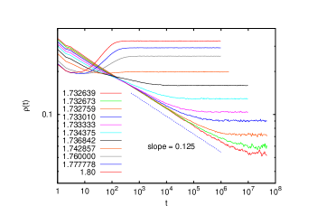
Figure 21: (Color online) Activity densities for supercritical FES systems, large enough to have negligible finite size effects. Initial configurations were chosen according to scheme A. The numbers in the legend indicate $\langle z\rangle$ (top curve has largest $\langle z\rangle$)

.

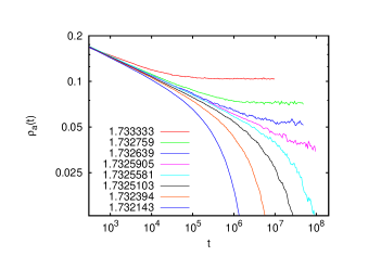
Figure 22: (Color online) Panel a: Activity densities for near critical FES systems. Initial conditions used scheme A, and lattices are large enough to have negligible finite size effects. The numbers in the legend indicate $\langle z\rangle$ (top curve has largest $\langle z\rangle$). Panel b: Data collapse obtained by plotting $t^{1/8}\rho_{a}(t)$ against $z_{c}-\langle z\rangle t^{\nu_{t}}$ with $\nu_{t}=21/40$. There are altogether 27 curves overlaid in this plot, for $\langle z\rangle$ ranging from 1.7143 to 1.7391.

Results obtained with these two schemes are shown in Fig. 20. There we used a large enough lattice ($L\approx 2^{15}$) and $\langle z\rangle$ sufficiently close to $z_{c}$ that we expect a pure power law for large $t$. Both schemes lead indeed to the same power law

$$\rho_{a}(t)\sim t^{-\theta}\;,\quad\theta=1/8\pm 0.002.$$ (30)

On the other hand, both schemes show corrections for intermediate $t$. For scheme A they seem to be a simple power law, but for B they are more complicated: There is a depletion for $10<t<10^{3}$ which indicates that declaring half of the $z_{i}=2$ sites in the NCS as unstable is indeed a too violent perturbation. This is even more pronounced for supercritical simulations, where scheme B gives very deep minima for intermediate $t$ (see Fig. 21). We thus conclude that scheme A gives, in spite of showing substantial finite-$t$ corrections, more reliable results that are easier to interpret. Final results are shown in Fig. 22. Panel a shows $\rho_{a}(t)$ against $t$ for a few selected near-critical values of $\langle z\rangle$, while panel b shows a collapse plot for the entire set of data in a rather wide range of $\langle z\rangle$. The structure near the the origin is due to the finite-time corrections mentioned above. Apart from that we see a perfect data collapse, indicating that indeed $\theta=1/8$ and

$$\nu_{t}=40/21.$$ (31)

Notice that Eq. (28) can now be written as $\delta+\eta+\theta=1/z$, in which form it is just the generalized hyperscaling relation for systems with multiple absorbing states proposed in Mendes .

III.5 Bulk driven open systems

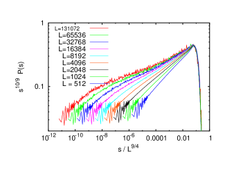
Figure 23: (Color online) Log-log plot of $s^{10/9}P(s,L)$ against $s/L^{9/4}$ for bulk driven open systems. In panel (a) the driving is uniformly distributed over the entire region $[1,L]$. while in panel (b) the center sites are driven. In both cases we see huge violations of scaling, which are biggest for uniform driving.

As we just discussed, the statistical properties of the stationary state are identical to those for boundary driving, thus we only have to discuss here the properties of avalanches. We again expect the scaling law Eq. (9) to hold, with the same exponent $D$. But $\tau$ should now be different Christ:2004a , because now $\langle s\rangle\sim L^{2}$. Assuming Eq. (9) we obtain

$$\tau_{\rm bulk}=2-2/D=10/9.$$ (32)

This should hold for any open system with large $L$, where stress is added at sites far from the boundaries. We shall discuss later the case where stress is added only at the center region, but let us first discuss the case of uniform driving which was considered e.g. in Malthe ; Christ:2004a .

In this case, the stress is not always added at sites far from the boundary, and corrections to scaling could be large, but the scaling could hold nevertheless. To test this, we plotted in Fig. 23a $s^{10/9}P(s,L)$ against $s/L^{9/4}$. If scaling were perfect, this would lead to a perfect data collapse. This is obviously not true (thus the fact that some avalanches start near a boundary is not negligible), but it seems to become true in the limit $L\to\infty$. In any case, both the position and the height of the peak scale in the right way. This means that avalanches starting near the boundaries don’t contribute to the peak, as we should expect.

More interesting is the case of center driving, because there we expect cleaner scaling than in case of uniform driving – although not as clean as for boundary driving. This is indeed seen in Fig. 23b, but the improvement over uniform driving is rather modest.

Both for center driving and for uniform driving we also measured moments of $T$. Ratios $\langle T^{k}\rangle/\langle T^{k-1}\rangle$ showed now clean power laws for both $k=2$ and $k=3$, with exponent $z=1.426(5)$, consistent with the previous estimate. But, in contrast to boundary driving, also $\langle T\rangle$ showed a power law with exponent $1.19(1)$.

Finally we show in Fig. 24 results for the temporal evolution of avalanches similar to those shown in Fig. 11 for the boundary driven case. Again these data show much poorer scaling. The only curve that shows a convincing power law is that for $R(t)$ (which is now defined as the root mean square distance), and which clearly shows the same value for the dynamical exponent $z$. The exponents $\delta$ and $\eta$ are clearly different from those for boundary driven systems. In view of the large deviations from scaling, the estimates

$$\delta_{\rm bulk}=7/40\;,\quad\eta_{\rm bulk}=2/5$$ (33)

seem not very well justified by the data alone, but they are consistent with the fixed-energy results presented in the last subsection.

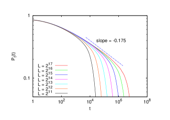
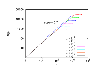
Figure 24: (Color online) Log-log plot of $P_{t}(t,L)$ (panel a), $N(t,L)$ (panel b), and $R(t,L)$ (panel c) for center driven systems, similar to Fig. 11 for boundary driven avalanches. The straight lines indicate power laws in the central (scaling) region.

IV Mapping onto an interface model

Following Paczuski , we define an interface without overhangs by identifying its height $H(i,t)$ with the number of topplings up to (and including) time $t$. Alternatively Pruessner , we could define another interface with height $h(i,t)$ such that $h(i,t)$ is the number of stress units received by topplings from its neighboring sites. The two heights are related by Pruessner

$$h(i,t)=H(i-1,t)+H(i+1,t).$$ (34)

On the other hand, the evolution of $z_{i}$ can be written as

$$z_{i,t}-z_{i,0} = h(i,t)-2H(i,t)$$ (35)

$$= H(i-1,t)+H(i+1,t)-2H(i,t)$$

$$\equiv \partial^{2}_{i}H(i,t),$$

where $\partial^{2}_{i}$ is the discrete Laplacian. Finally, the number of topplings at $(i,t)$ is just a (random) function of $z_{i,t}$,

$$H(i,t+1)-H(i,t)=\sigma(z_{i,t})$$ (36)

with

$$\sigma(z)=\begin{cases}0&\quad\text{if }z\leq 1\\ 1&\quad\text{if }z>2\\ 0\;\;\text{or}\;\;1&\quad\text{with probability 1/2, if }z=2.\end{cases}$$ (37)

The last equations can be summarized as

$$\partial_{t}H(i,t)=\partial^{2}_{i}H(i,t)+\eta[i;H(i-1,t),H(i,t),H(i+1,t)]$$ (38)

with $\eta(x,y)=\sigma(x)+x-y$. This looks formally like the qEW equation Natter

$$\partial_{t}H(i,t)=\partial^{2}_{i}H(i,t)+\eta[i;H(i,t)]$$ (39)

except that in the latter the noise $\eta$ depends only on $i$ and $H(i,t)$. In Eq. (38), in contrast, there is explicit dependence on the stresses $z_{i,t}$. Note that in Eq. (38), unlike the qEW equation, the noise depends not only on a quenched variable at the site in question, but also on the curvature of the interface .

Thus, the Oslo model is not exactly equivalent to the standard qEW model based on the interface $H$, where the noise correlations are

$$\langle\eta(t,H)\eta(t^{\prime},H^{\prime})\rangle=\delta_{t,t^{\prime}}\delta_{H,H^{\prime}}.$$ (40)

Because $h$ is an explicit function of $H$ due to Eq. (34), this is also true if $H$ is exchanged by $h$, in contrast to what is claimed in Pruessner . It is also not true that $H$ and $h$ have different scaling properties, as was claimed in Pruessner ; Bona:2007 . As should be clear from Eq. (34), and as will be verified numerically, they show exactly the same scaling.

Let us finally discuss the interface interpretation of the original Oslo model which is driven from its left border. As shown in Paczuski , this corresponds to an interface that is prevented from being pinned by pulling slowly up the leftmost point. Consider the case where the interface is at its left end pulled by an amount $H(1,t)\gg L$, after which the pulling stops. In this case the left hand side of Eq. (39) vanishes, and it can be written as

$$H(i+1,t)=2H(i,t)+\eta(i,H(i,t))-H(i-1,t),$$ (41)

showing that the evolution in the variable $i$, considered as a ’time’-evolution, is Markovian. Moreover, since the noise is assumed to be zero in average, the averaged heights satisfy simply $\partial^{2}_{i}\langle H(i,t)\rangle=0$, showing that the height profile is just linear.

Figure 25: (Color online) Roughness $W$ of interfaces constructed from the FES Oslo model, on lattices with density $\langle z\rangle=473/273=1.732601$ and lattice sizes which are multiples of 273. Panel (a) shows the raw data, while panel (b) shows a data collapse obtained by plotting $L^{-\alpha_{\rm qEW}}W$ against $t/L^{z}$. In this and the following two figures, averages are taken over all runs, those which are still active at time $t$ and those which had already died. If we had excluded the latter from the averages, interfaces would be slightly less rough (roughness increases sharply immediately before interfaces get pinned), but this would not affect their scaling (while it would affect the scaling of average height).

We have already discussed the main idea of the mapping on the qEW model, and we have already given the numerical value of the exponent, called usually $\theta$ in the qEW model, that describes how the average interface velocity increases with the distance from the critical point. Here we shall discuss more relations of this type. An annoying problem in doing so is the fact that equivalent exponents are given different names in the Oslo and qEW interpretations. We shall deal with it by adding a subscript “qEW” to all qEW exponents, e.g. $v\sim(F-F_{c})^{\theta_{\rm qEW}}$ (notice that $z$ and $\nu$ are defined in the same way in the Oslo and qEW models). In the following we shall discuss only the behavior exactly at the critical point, which we approximate to sufficient precision as $\langle z\rangle=473/273=1.732601$. As we said in Sec. 2, there are two slightly different mappings from the Oslo model onto the interface model. In the first, $h(i,t)$ is the number of stress units received at site $i$ up to (and including) time $t$, while in the other $H(i,t)$ is the number of topplings.

Let us first discuss how the global roughness of an interface $h$ of base $L$ increases at the critical force with time. The roughness is defined as the square root of $W^{2}=\langle(\Delta h(t))^{2}\rangle$, where brackets stand for an ensemble average and

$$(\Delta h(t))^{2}=\frac{1}{L}\sum_{i}h(i,t)^{2}-[\frac{1}{L}\sum_{i}h(i,t)]^{2}$$ (42)

Results are shown in Fig. 25. They demonstrate the well known behavior

$$W(t,L)=t^{\beta_{\rm qEW}}f(t/L^{z})=L^{\alpha_{\rm qEW}}\tilde{f}(t/L^{z})$$ (43)

with $\beta_{\rm qEW}=1-\theta=7/8$ and $\alpha_{\rm qEW}=z\beta_{\rm qEW}=5/4$. The most precise previous estimates of the exponents were in Song-Kim and Ferrero . They are, respectively, $\beta_{\rm qEW}=0.871(3)\;[0.872(3)],\;\alpha_{\rm qEW}=1.250(3)\;[1.250(3)]$ and $z=1.440(15)\;[1.443(7)]$, and are somewhat less precise than our estimates.

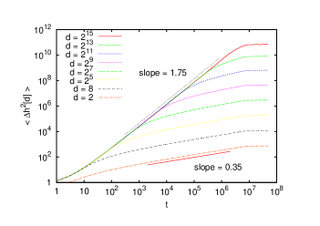
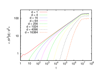
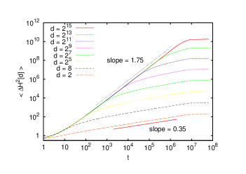
Figure 26: (Color online) (a) Log-log plot of local squared roughnesses of interfaces constructed from the FES Oslo model, on lattices with density $\langle z\rangle=473/273=1.732601$ and size $L=131040$. The straight lines indicate the anomalous roughening power laws. Panel (b) shows the same data, but divided by $d^{2}$. According Eq. (44) one should see a data collapse for $d\ll t^{1/z}\ll L$. There is indeed a perfect collapse for $t\approx 10^{6}$, if the largest distances $d$ are discarded. Panel (c), finally, is analogous to panel (a) but shows data for the alternative interface definition that is based on number of topplings instead of received units of stress.

Since $\alpha_{\rm qEW}>1$ (critical qEW interfaces are “superrough”), the local slope of a critical interface cannot be bounded Lesch-Tang , and local roughnesses (i.e. roughnesses measured on a length scale $d\ll L$ must still increase for times at which an interface of total length $d$ would already be pinned. Thus the roughness of a part of length $d$ of an interface of base $L\gg d$ satisfies “anomalous scaling” Sarma

$$W(d;t,L)\sim\begin{cases}t^{\beta_{\rm qEW}}&\quad\text{for }\;t\ll d^{z}\\ d^{\alpha_{\rm loc}}L^{\alpha_{\rm qEW}-\alpha_{\rm loc}}&\quad\text{for }\;d\ll L\ll t^{1/z}\\ d^{\alpha_{\rm loc}}t^{(\alpha_{\rm qEW}-\alpha_{\rm loc})/z}&\quad\text{for }\;d\ll t^{1/z}\ll L,\end{cases}$$ (44)

where $\alpha_{\rm loc}$ is a new exponent which for consistency must be $\leq 1$. In Sarma , $\alpha_{\rm qEW}-\alpha_{\rm loc}$ was called $\kappa/2$, but we shall follow Lopez ; Bona:2007 and define

$$\kappa=\frac{\alpha_{\rm qEW}-\alpha_{\rm loc}}{z},$$ (45)

so that the scaling for intermediate times reads now

$$W\sim d^{\alpha_{\rm loc}}t^{\kappa}\quad\text{for }\;d\ll t^{1/z}\ll L.$$ (46)

If the Oslo model is in the qEW universality class, the interfaces it is mapped onto must also satisfy these scaling relations. In order to test this, we show local roughnesses of $h(i,t)$ in panels (a) and (b) of Fig. 26, while local roughnesses of $H(i,t)$ are shown in panel (c). All three panels in Fig. 26 show data for $L=131040$ and $\langle z\rangle=473/273$. Panel (a) shows a log-log plot of the square of the roughness against $t$. Each curve corresponds to a distance $d=2^{k},\;k=1,3,5,\ldots,15$ over which the roughness is computed. It is defined as $W^{2}(d;t,L)=\langle[h(i,t)-h(i+d,t)]^{2}\rangle$. We see clearly the two scaling laws $W(d;t,L)\sim t^{\beta_{\rm qEW}}$ for $t<d^{z}$ with $\beta_{\rm qEW}=0.875$, and Eq. (46) with $\kappa=7/40\pm 0.01$. Notice that the latter holds for all $d$, even for $d=1$ (not shown). Panel (b) shows the same data, but in order to see more clearly the value of $\alpha_{\rm loc}$ we divided the roughness by $d$. We see a perfect data collapse for $t\gg 1$ and $d\ll t^{1/z}$, which implies that

$$\alpha_{\rm loc}=1,$$ (47)

in agreement with our estimate $\kappa=7/40$. Finally, panel (c) of Fig. 26 is completely analogous to panel (a), except that it shows roughnesses of the interface $H(i,t)$ which is obtained from the number of topplings instead of the number of units received by a site. It clearly demonstrates that both interface definitions lead to the same scaling.

Our result $\alpha_{\rm loc}=1$ is obtained in many different 1-d interface models Sarma ; Lopez , but to our knowledge it cannot be derived analytically for the qEW model. Previous numerical estimates Lopez-Rod agree with it. On the other hand, our finding that the interfaces $H(i,t)$ and $h(i,t)$ satisfy the same scaling disagrees with claims made in Pruessner ; Bona:2007 . In particular, we find for both the same exponent $\kappa$. This value agrees with what is called “A scaling” in Bona:2007 . In contrast to claims made in Bona:2007 , the Oslo model seems incompatible with what is called there “B scaling”.

V Conclusions

Part of the motivation for the present work was the observation that natural critical state in the Oslo model is models are hyperuniform. On the one hand this suggests that transients in simulations could be cut short by starting from very uniform initial configurations. This was indeed found, and it allowed the simulation of much bigger systems than previously possible.

On the other hand it suggested that – if the hyperuniformity is strong enough – the conserved field in sandpile models can be considered as rigid and non-fluctuating, in which case these models would be in the same universality class as directed percolation. We find that this is not so (see also Dick:2015 ). Instead, we find compelling evidence that the 1-dimensional Oslo model is in the same universality class as the qEW (or linear interface) model. This had been a long-standing conjecture, but it had been repeatedly doubted due to contradictory numerical results. One main reason for these numerical problems was precisely that hyperuniformity had not been taken into account. In a forthcoming paper forthcoming , we will discuss some other Oslo type models with directed particle transfer rules on two-dimensional lattices, which turn out to correspond to an Edwards-Wilkinson interface model with annealed noise.

An unexpected outcome of this work is that the vastly improved simulations (made possible in part by judicious choices of initial conditions) suggest that the critical exponents of the 1-d Oslo model (and, more importantly, also the 1-d qEW model) are simple rational numbers. For some exponents this had already been conjectured before, but not (to our knowledge) for the dynamical and hyperuniformity exponents, and for the exponent $\sigma$ (see Eq. (5) describing the stress profile in the case of open boundaries. Also, these exponents fall outside the infinite series of discrete rational exponents recently found for 1-d stochastic models schutz . Of course, in the same study, well-behaved models where the dynamical exponent is the golden mean, i.e. an irrational value have also been discussed. So, while the critical exponents do not have to be rational, we note that most soluble models so far have found rational critical exponents. Showing that these conjectured values are actually correct remains a challenge.

Our finding that the 1-d Oslo model is in the qEW universality class suggests of course that the same could be true for other stochastic sandpile models, and for SOC models with conserved fields in higher dimensions. This does not invalidate our earlier argument about instability of the Manna model fixed point under suitable perturbation to DP. All this says is that adding this kind of perturbation (say adding a small probability of $z_{c}$ being set to $3$, $z_{c}=2$ is the deterministic sandpile) does not constitute such a relevant perturbation. One possibility is that if in the toppling process, we add randomness also in where the transferred particles may go ( as in the original Manna model), then the critical behavior of the model may change. This can occur, because with such randomness present, there is a much larger variation of the number of topplings at different sites in an avalanche. In fact, other stochastic 1-d sandpile models (like the Maslov-Zhang model Maslov-Zhang or the continuous Manna model BBBMH ) appear to have critical exponents different from to the Oslo model studied here. Further studies are needed to clarify this point.

- (1) P. Bak, C. Tang, and K. Wiesenfeld, Phys. Rev. Lett. 59, 381 (1987).
- (2) E.V. Ivashkievich, D.V. Ktitarev, and V.B. Priezzhev, Physica A 209, 347 (1994).
- (3) D.V. Ktitarev, S. Lübeck, P. Grassberger, and V.B. Priezzhev, Phys. Rev. E 61, 81 (2000).
- (4) D. Dhar, Physica A 239 29(2006).
- (5) F. Redig, Les Houches, Volume 83, 2006, Pages 657–659, 661–729.
- (6) L. Levine and J. Propp, Notices of the AMS, 57 976 (2010).
- (7) C Tebaldi, M. De Menech, and A.L. Stella, Phys. Rev. Lett 83 3952 (1999).
- (8) A. Benhur and O. Biham, Phys. Rev. E 53 R1317 (1996).
- (9) S.S. Manna, J. Phys. A 24, L363 (1991).
- (10) V. Frette, K. Christensen, A. Malthe-Sørensen, J. Feder, T. Jøssang, and P. Meakin, Nature 379, 49 (1996).
- (11) Y.-C. Zhang, Phys. Rev. Lett. 63, 470 (1989).
- (12) S. Maslov and Y.-C. Zhang, Physica A 223, 1 (1996).
- (13) M. Rossi, R. Pastor-Satorras, and A. Vespignani, Phys. Rev. Lett. 85, 1803 (2000).
- (14) P.K. Mohanty and D. Dhar, Phys. Rev. Lett. 89,104303 (2002).
- (15) P.K. Mohanty and D. Dhar, Physica A 384, 34 (2007).
- (16) M. Basu, U. Basu, S. Bondyopadhyay, P.K. Mohanty, and H. Hinrichsen, Phys. Rev. Lett. 109, 15702 (2012).
- (17) C. Tang and P. Bak, Phys. Rev. Lett. 60, 2347 (1988).
- (18) C. Tang and P. Bak, J. Stat. Phys. 51, 797 (1988).
- (19) P. Grassberger and S.S. Manna, J. Physique 51, 1077 (1990).
- (20) H. Hinrichsen, Advances in Physics 49, 815 (2000).
- (21) In the ‘random subtraction’ version of the fixed-energy BTW model in Chessa , e.g., simulations were done at slightly subcritical densities (so that avalanches died), and new avalanches were triggered by moving one of the sand grains to an random arbitrarily far away site. It is not clear that the steady state produced this way is the same as what would be produced if the grain was moved only to nearest neighbor site.
- (22) V. Frette, Phys. Rev. Lett. 70 (1993) 2762; K. Christensen, A. Corral, V. Frette, J. Feder, and T. Jossang, Phys. Rev. Lett., 77 ( 1996) 49.
- (23) D. Dhar, Physica A,340 (2004) 535.
- (24) D. Hexner and D. Levine, Phys. Rev. Lett. 114, 110602 (2015).
- (25) S.B. Lee, Phys. Rev. E 89, 060101 (2014).
- (26) R. Dickman and S.D. da Cunha, Phys. Rev. E 92, 020104(R) (2015).
- (27) S. Torquato and F.H. Stillinger, Phys. Rev. E 68, 041113 (2003).
- (28) A. Gabrielli, M. Joyce, and F.S. Labini, Phys. Rev. D 65, 083523 (2002).
- (29) A. Fey, L. Levine, and D. Wilson. Phys. Rev. E 82, 031121 (2010).
- (30) The latter are the most “natural” b.c.’s if we concentrate on the . Although a different b.c. at the right boundary was used in Oslo , we call Eq. (2) ‘the original Oslo model’, since the difference is irrelevant for scaling.
- (31) K. Christensen, N.R. Moloney, O. Peters, and G. Pruessner, Phys. Rev. E 70, 067101 (2004).
- (32) A. Vespignani, R. Dickman, M.A. Muñoz, and S. Zapperi, Phys. Rev. E 62, 4564 (2000).
- (33) A. Chua and K. Christensen, e-print arXiv:cond-mat/0203260 (2002).
- (34) K. Christensen, A. Corral, V. Frette, J. Feder, and T. T. Jossang, Phys. Rev. Lett. 77, 107 (1996).
- (35) G. Pruessner and H.J. Jensen, Phys. Rev. Lett. 91, 244303 (2003).
- (36) M. Paczuski and S. Boettcher, Phys. Rev. Lett. 77, 111 (1996).
- (37) K. Christensen, Physica A 340, 527 (2004).
- (38) J.A. Bonachela, Universality in Self-Organized Criticality, PhD thesis, Univ. Granada (2008).
- (39) R. Dickman, M. Alava, M.A. Munoz, J. Peltola, A. Vespignani, and S. Zapperi, Phys. Rev. E 64, 056104 (2001).
- (40) R. Dickman, T. Tome and M.J. de Oliveira, Phys. Rev. E 66, 016111 (2002).
- (41) R. Dickman, Phys. Rev. E 66, 036122 (2002).
- (42) R. Dickman, Phys. Rev. E 76, 036131 (2006).
- (43) J. Kockelkoren and H. Chaté, e-print arXiv:cond-mat/0306039 (2003).
- (44) J.J. Ramasco, M.A. Muñoz, and C.A. da Silva Santos, Phys. Rev. E 69, 045105(R) (2004).
- (45) S. Lübeck, Int. J. Mod. Phys B 18, 3977 (2004).
- (46) E. Fiore and M.J. de Oliveira, Braz. J. Phys. 36, 218 (2006).
- (47) H. Leschhorn, Physica A 195, 324 (1993).
- (48) O. Duemmer and W. Krauth, Phys. Rev. E 71, 061601 (2005).
- (49) J.M. Kim and H. Choi, J. Kor. Phys. Soc. 48, S241 (2006);
- (50) H.S. Song and J.M. Kim, J. Kor. Phys. Soc. 53, 1802 (2008).
- (51) A. Corral and M. Paczuski, Phys. Rev. Lett. 83, 572 (1999).
- (52) E.E. Ferrero, S. Bustingorry, and A.B. Kolton, Phys. Rev. E 87, 032122 (2013).
- (53) S.B. Lee, J. Kor. Phys. Soc. 55, 2339 (2009); 60, 559 (2012).
- (54) J.F.F. Mendes, R. Dickman, M. Henkel, and M. Ceu Marques, J. Phys. A: Math. Gen. 27, 3019 (1994).
- (55) A. Malthe-Sørensen, Phys. Rev. 59, 4169 (1999).
- (56) G. Pruessner, Phys. Rev. E 67, 030301 (2003).
- (57) T. Nattermann, S. Stepanov, L.H. Tand, and H. Leschhorn, J. Physique II 2, 1483 (1992).
- (58) J.A. Bonachela, H. Chaté, I. Dornic, and M.A. Muñoz, Phys. Rev. Lett. 98, 155702 (2007).
- (59) H. Leschhorn and L.-H. Tang, Phys. Rev. Lett. 70, 2973 (1993).
- (60) S. Sarma, S.V. Ghaisas, and J.M. Kim, Phys. Rev. E 49, 122 (1994).
- (61) J.M. López, Phys. Rev. Lett. 83, 4594 (1999).
- (62) J.M. López and M.A. Rodriguez, J. Physique I France 7, 1191 (1997).
- (63) Mohanty, Dhar, Grassberger, in preparation.
- (64) V. Popkov, A. Schadschneider, J. Schmidt, G. M. Schütz, Proc. Nat. Acad. Sc. (USA) vol. 112, no. 41, 12645-12650 (2015).
- (65) A. Chessa, E. Marinari, and A. Vespignani, Phys. Rev. Lett. 80, 4217 (1998).