Influence of the Coulomb interaction on the exchange coupling in granular magnets

Abstract

We develop a theory of the exchange interaction between ferromagnetic (FM) metallic grains embedded into insulating matrix by taking into account the Coulomb blockade effects. For bulk ferromagnets separated by the insulating layer the exchange interaction strongly depends on the height and thickness of the tunneling barrier created by the insulator. We show that for FM grains embedded into insulating matrix the exchange coupling additionally depends on the dielectric properties of this matrix due to the Coulomb blockade effects. In particular, the FM coupling decreases with decreasing the dielectric permittivity of insulating matrix. We find that the change in the exchange interaction due to the Coulomb blockade effects can be a few tens of percent. Also, we study dependence of the intergrain exchange interaction on the grain size and other parameters of the system.

magneto-electric effect, multiferroics, Coulomb blockade, granular:

1 Introduction

Physics of granular ferromagnets (GFM) combines numerous phenomena appearing at different length and energy scales. This makes GFM a complicated object suitable for investigation of fundamental effects and their mutual influence [1, 2, 3, 4, 5, 6, 7, 8, 9, 10, 11, 12, 13, 14]. Disorder combined with strong Coulomb interaction leads to peculiar dependence of the conductivity of granular metals on temperature [15]. The Coulomb blockade strongly affects superconductivity in granular superconductors [16, 17, 18]. Granular ferroelectrics demonstrate the metal-insulator transition driven by temperature and electric field [19, 20, 21]. In granular materials with small grains the size quantization effects become important [15]. Besides, these materials are known as good candidates for various applications [22, 23, 24].

In this manuscript we study magnetic properties of granular ferromagnets - materials with ferromagnetic (FM) metallic grains embedded into insulating matrix. The magneto-dipole (MD) [25, 26, 27, 28] and the exchange interactions [29, 30, 31, 32, 33] are the main intergrain coupling mechanisms in GFM. Long range MD interaction leads to the formation of super spin glass (SSG) state in the system. Depending on its sign the short range exchange coupling causes the formation of either super ferromagnetic (SFM) state or the SSG state. In addition to the interparticle interaction the magnetic anisotropy of individual grains influences the properties of the GFM leading to “blocking” phenomena [34, 35, 36, 37].

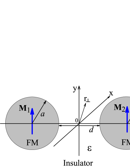
Figure 1: (Color online) Two FM metallic grains with radius $a$ and intergrain distance $d$ embedded into insulating matrix with dielectric constant $\varepsilon$. $\bi M_{1,2}$ stands for grain magnetic moment. (x,y,z) is the coordinate system. $\bi r_{\perp}$ is the radius vector in the (x,y) plane.

For well separated grains the interparticle coupling is weak and the properties of GFM are defined by the single particle magnetic anisotropy. This situation is well studied theoretically and experimentally. As the grains move closer to each other the MD interaction becomes important. For even smaller distances, of the order of 1 nm, the exchange coupling becomes crucial. The influence of the exchange interaction on macroscopic magnetic state of GFM is understood using the Heisenberg model, $\sum_{ij}J_{ij}(\bi M_{i}\bi M_{j})$ [31, 38, 37], where summation is over the all nearest neighbor grain pairs in the whole GFM, $\bi M_{i}$ is the magnetic moment of grain $i$ and $J_{ij}$ is the exchange coupling constant for grain pair {$ij$}. However, the microscopic theory of the exchange interaction between magnetic grains (constant $J_{ij}$) is still lacking. The understanding of the intergrain exchange interaction is mostly based on the Slonczewski theory developed for coupling of infinite FM layers separated by the insulating layer [39, 40]. According to Slonczewski the interlayer exchange coupling appears due to virtual electron hopping (or tunnelling) between FM leads. This theory does not take into account the many-body effects and charge quantization phenomena. The influence of many-body effects on the ground magnetic state and transport properties of solid state systems is a long standing fundamental problem appearing in a broad range of physical problems. In nanoscale granular systems the many-body effects due to Coulomb interaction between electrons become crucial [15]. In particular, these effects influence the electron transport in granular metals [15], ferromagnets [41], superconductors [42] and ferroelectrics [19, 20]. In this paper we show another example of importance of many-body effects in granular systems. We develop a theory of the exchange interaction between FM nanograins embedded into insulating matrix by taking into account the Coulomb blockade effects (see figure 1) and show that in granular systems the matrix dielectric constant and the grain size influence the intergrain exchange interaction. Note that the typical grain sizes considered in this paper is in the range of few nms with thousands of atoms. The Coulomb blockade is important for such grains. At the same time the grains can be treated as bulk metal neglecting surface and size quantization effects such as in magnetic clusters made of several atoms.

Note that experimental realization of the GFM with the intergrain exchange coupling meets a number of difficulties. The most complicated task is the control of the intergrain distance on the scale of 1 nm. Nonetheless, several studies observed the intergrain exchange interaction of FM type with rather large value [29, 30, 31].

The paper is organized as follows. We summarize our main results in Sec. 2. We introduce the model to study the exchange interaction between two magnetic grains in Sec. 3. In Sec. 4 and 5 we calculate the exchange interaction between two ferromagnetic grains embedded into insulating matrix. In Sec. 6 we analyze the dependence of the intergrain exchange interaction on the system parameters. We discuss validity of our model in Sec. 7.

2 Main results

Here we summarize our main findings.

1) We develop a theory of the exchange interaction between FM metallic grains embedded into insulating matrix by taking into account the Coulomb blockade effects. We show that beside height and thickness of the insulating barrier the intergrain exchange coupling depends on the dielectric properties of the spacer. This additional dependence occurs due to the Coulomb blockade effects (see figure 3). The FM coupling decreases with decreasing the dielectric permittivity of insulating matrix.

2) We predict the behavior of intergrain exchange interaction $J$ as a function of grain size $a$. On one hand increasing the grain size leads to the linear increase of the interaction due to geometrical factor, $J\sim a$. On the other hand decreasing the grain size leads to the enhancing of the Coulomb blockade and decreasing the FM contribution to the exchange coupling. Finally, the exchange interaction decays faster than the first power of $a$ with decreasing the grain size.

3) We find that the Coulomb blockade influences the intergrain exchange coupling strongly if: i) the Fermi momentum is not too large and ii) the spin subband splitting is of the order of the Fermi energy (see figure 4).

4) We show that the impact of the Coulomb blockade also depends on the barrier thickness and height: The thicker and the lower the barrier - the stronger the Coulomb blockade effect.

3 The model

We consider two identical FM grains with radius $a$ and the distance between the grain surfaces being $d$ (see figure 1). The Hamiltonian describing delocalized electrons in the system has the form

$$\hat{H}=\hat{H}_{\mathrm{sp}}+\hat{H}_{\mathrm{C}},$$ (1)

where single particle Hamiltonian $\hat{H}_{\mathrm{sp}}=\sum_{i}(\hat{K}(\bi r_{i})+\hat{U}_{1}(\bi r_{i})+\hat{U}_{2}(\bi r_{i})+\hat{H}_{1\mathrm{m}}(\bi r_{i}))+\hat{H}_{2\mathrm{m}}(\bi r_{i}))$ consists of kinetic energy $\hat{K}$, potential energy $\hat{U}_{1,2}$ and exchange interaction between delocalized and localized electrons, $\hat{H}_{1,2\mathrm{m}}$. Summation is over $2n_{0}$ electrons in the system, where $n_{0}$ is the number of electrons in each grain. The single particle potential energy inside the grain (1) is $\hat{U}_{1}=-U$ ($U>0$) and $\hat{U}_{1}=0$ outside the grain (1), $\hat{U}_{2}=-U$ inside the grain (2) and $\hat{U}_{2}=0$ outside the grain (2). We consider FM and AFM configurations of grain magnetizations. Therefore magnetic interaction has the form, $\hat{H}_{1,2\mathrm{m}}=-J_{\mathrm{sd}}\hat{\sigma}_{z}M_{1,2}$ inside the grains, with $M_{1,2}=\pm 1$, $\hat{\sigma}_{z}$ being the Pauli matrix and $\mathit{J}_{\mathrm{sd}}$ being the coupling constant of the s-d interaction responsible for spin subband splitting of conduction electrons. The energy profiles for spin up and spin down subbands are shown in figure 2 for AFM configuration of grain magnetic moments.

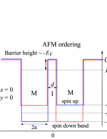
Figure 2: (Color online) Schematic picture of potential energy profiles for electron with spin “up” (red line) and spin “down” (blue line) states for AFM configuration of grain magnetic moments. Profiles are slightly shifted with respect to each other for better viewing. Zero energy corresponds to the top of energy barrier for electrons in the insulator. Symbols M and I stand for metal and insulator, respectively. All other notations are defined in the text.

We introduce a single particle Hamiltonian for each grain, $\hat{H}^{\mathrm{g}}_{1,2}=\hat{K}+\hat{U}_{1,2}+\hat{H}_{1,2\mathrm{m}}$, with eigenfunctions $\psi_{i}^{s}$ and $\phi_{i}^{s}$ for grain (1) and (2), respectively. Here we note that the single particle Hamiltonian of two grains is not the sum of $\hat{H}^{\mathrm{g}}_{1}$ and $\hat{H}^{\mathrm{g}}_{2}$. The subscript $i$ stands for orbital state and the superscript $s$ denotes the spin state in a local spin coordinate system related to magnetization of corresponding grain. Due to grains symmetry the wave functions are symmetric

$$\psi^{s}_{i}(x,y,z)=\phi^{s}_{i}(x,y,-z).$$ (2)

Since we consider identical grains, energies of these states are equal and denoted $\epsilon_{i}^{s}$.

Functions $\psi_{i}^{s}$ are orthogonal to each other and normalized, $\langle\psi_{i}^{s}|\psi_{j}^{s^{\prime}}\rangle=\delta_{i,j}\delta_{s,s^{\prime}}$ and $\langle\phi_{i}^{s}|\phi_{j}^{s^{\prime}}\rangle=\delta_{i,j}\delta_{s,s^{\prime}}$. However, functions $\psi_{i}^{s}$ and $\phi_{i}^{s}$ are not orthogonal to each other, $\langle\phi_{i}^{s^{\prime}}|\psi_{j}^{s}\rangle=P^{s}_{ij}\delta_{s,\pm s^{\prime}}$ (symbol $+$ stands for FM and $-$ is for AFM configurations). We assume that the barrier between the grains is high enough such that the wave functions overlap integral, $P^{s}_{ij}$ is small, $P^{s}_{ij}\ll 1$. The wave functions $\psi$ and $\phi$ exponentially decay outside the grains with some characteristic length scale $1/\varkappa$ ($\psi\sim\rme^{-\varkappa r_{1}}$ and $\phi\sim\rme^{-\varkappa r_{2}}$, where $r_{1}(r_{2})$ is the distance from the centre of the corresponding grain). Due to the exponential decay the overlap is small and can be estimated as $P^{s}_{ij}\sim\rme^{-\varkappa d}$. At the Fermi level $E_{\mathrm{F}}$ (in our consideration $E_{\mathrm{F}}<0$, see figure 2) the inverse decay length is $\varkappa_{0}\approx\sqrt{-2m_{\mathrm{e}}E_{\mathrm{F}}/\hbar^{2}}$. Thus, increasing the barrier thickness or the barrier height one can control the smallness of the overlap integral. Below we use, $p=\rme^{-\varkappa_{0}d}$, as the small parameter in the problem. We neglect all states with energies $\epsilon^{s}_{i}>0$ since these states are fully delocalized.

The zero-order many-particle wave function $\Psi_{0}$ corresponds to the system state with all single particle states $\psi^{s}_{i}$ and $\phi^{s}_{i}$ with energies $\epsilon^{s}_{i}<E_{\mathrm{F}}$ being filled and with all states above $E_{\mathrm{F}}$ being empty (see Appendix C for details). The creation and annihilation operators are $\hat{a}^{s+}_{i}$ and $\hat{a}^{s}_{i}$ in grain (1), and $\hat{b}^{s+}_{i}$ and $\hat{b}^{s}_{i}$ in grain (2). We introduce here the excited wave functions $\Psi_{ij}^{s}=\hat{a}^{s^{\prime}+}_{i}\hat{b}^{s}_{j}\Psi_{0}$ and $\tilde{\Psi}_{ij}^{s}=\hat{b}^{s^{\prime}+}_{i}\hat{a}^{s}_{j}\Psi_{0}$ ($s^{\prime}=s$ for FM orientation of $\bi M_{1}$ and $\bi M_{2}$ and $s^{\prime}=-s$ for AFM configuration). We neglect states with two electrons being transferred between grains since these states have much larger Coulomb energy.

We use the simplest model for Coulomb interaction with diagonal elements only. The zero order wave function corresponds to the system state where both grains are neutral and the Coulomb energy is zero, $\langle\Psi_{0}|\hat{H}_{\mathrm{C}}|\Psi_{0}\rangle=0$. In the excited states $\Psi^{s}_{ij}$ and $\tilde{\Psi}^{s}_{ij}$ an electron is transferred from one grain into another. Therefore, the grains have opposite charges and the energy of the Coulomb interaction is $\langle\Psi_{ij}^{s}|\hat{H}_{\mathrm{C}}|\Psi_{ij}^{s}\rangle=\langle\tilde{\Psi}_{ij}^{s}|\hat{H}_{\mathrm{C}}|\tilde{\Psi}_{ij}^{s}\rangle=\tilde{\epsilon}_{\mathrm{c}}=e^{2}(C^{-1}-(2C_{\mathrm{m}})^{-1})$. This is just the classical electrostatic energy of two oppositely charged metallic spheres. Here $C$ is the single grain capacitance and $C_{\mathrm{m}}$ is the mutual capacitance of two grains. We can estimate the charging energy as $\tilde{\epsilon}_{\mathrm{c}}=e^{2}/(8\pi a\varepsilon\varepsilon_{0})$ for $d\approx 1$ nm and $a\in\left[1;10\right]$ nm, here $\varepsilon$ is the effective dielectric permittivity of GFM and $\varepsilon_{0}$ is the vacuum dielectric constant. We assume that the Coulomb interaction does not transfer electrons between grains, or the Coulomb-based hopping is negligible in comparison with the hopping due to kinetic energy. Thus, we have $\langle\Psi_{ij}^{s}|\hat{H}_{\mathrm{C}}|\Psi_{0}\rangle=\langle\tilde{\Psi}_{ij}^{s}|\hat{H}_{\mathrm{C}}|\tilde{\Psi}_{0}\rangle=\langle\Psi_{0}|\hat{H}_{\mathrm{C}}|\Psi_{ij}^{s}\rangle=\langle\tilde{\Psi}_{0}|\hat{H}_{\mathrm{C}}|\tilde{\Psi}_{ij}^{s}\rangle=0.$ This model for the Coulomb interaction is valid for metallic grains with large conductance [15, 43].

We will study two cases: 1) FM and 2) AFM alignment of grain magnetic moments. Both these configurations are collinear meaning that the single particle interactions $\hat{W}_{\mathrm{k}}$, $\hat{U}_{1,2}$ and $\hat{H}_{1,2\mathrm{mag}}$ are diagonal in the spin space.

Below we will find the energy of the system for FM ($E^{\mathrm{FM}}$) and AFM ($E^{\mathrm{AFM}}$) alignment and calculate the intergrain magnetic (exchange) interaction,

$$J=E^{\mathrm{AFM}}-E^{\mathrm{FM}}.$$ (3)

For $J>0$ the interaction between the grains is FM while for $J<0$ it is AFM. We consider the case of zero temperature and therefore neglect all inelastic transitions of electrons between grains due electron-phonon interaction. Thus, we take into account only co-tunneling processes neglecting sequential tunneling (see Sec. 7 for more details).

The Hamiltonian in (1) does not include the vector potential occurring due to magnetic field produced by the grains. This contribution is small in comparison with s-d exchange coupling and can be neglected. Also we neglect the MD interaction. On one hand this interaction was considered in numerous papers in the past. On the other hand the MD interaction is the long range interaction and thus its consideration for two grains only is meaningless. This coupling should be considered on the scale of whole granular magnet.

4 Single grain wave functions and matrix elements

We use the following approximate wave functions to calculate all matrix elements. Outside the grain the wave function corresponding to the wave vector $\bi k$ and the spin state $s$ is

$$\eqalign{\psi{k}^{s}(z,r_{\perp})\approx\frac{\tau k^{s}}{\sqrt{\Omega}}\exp\left(-\varkappa k^{s}\left(\frac{d}{2}+z+\frac{r_{\perp}^{2}}{2a}\right)\right)\rme^{\rmi\bi k_{\perp}\bi r_{\perp}},\cr\phi{k}^{s}(z,r_{\perp})\approx\frac{\tau^{s}k}{\sqrt{\Omega}}\exp\left(-\varkappa k^{s}\left(\frac{d}{2}-z+\frac{r_{\perp}^{2}}{2a}\right)\right)\rme^{\rmi\bi k_{\perp}\bi r_{\perp}}.}$$ (6)

Here $\tau{k}^{s}=\frac{2k_{z}}{k_{z}+\rmi\varkappa^{s}k}$ is the amplitude of the transmitted electron wave, $\bi k_{\perp}=(k_{x},k_{y},0)$, $\bi r_{\perp}=(x,y,0)$, $\Omega=4\pi a^{3}/3$ is the grain volume and $\varkappa^{s}k=\sqrt{2m_{\mathrm{e}}(U-s\mathit{J}_{\mathrm{sd}}-\hbar^{2}k^{2}_{z}/(2m_{\mathrm{e}}))/\hbar^{2}}$ is the inverse decay length. We introduce the following coordinates: $z$ is along the line connecting grain centres; $z=0$ is the symmetry point between the grains; $x$ and $y$ are perpendicular to $z$. For electron wave function inside the grains we have

$$\eqalign{\psi^{s}k(z,r_{\perp})\approx\frac{\rme^{\rmi k_{z}\left(\frac{d}{2}+z+\frac{r_{\perp}^{2}}{2a}\right)}+\xi^{s}k\rme^{-\rmi k_{z}\left(\frac{d}{2}+z+\frac{r_{\perp}^{2}}{2a}\right)}}{\sqrt{\Omega}}\rme^{\rmi\bi k_{\perp}\bi r_{\perp}},\cr\phi^{s}k(z,r_{\perp})\approx\frac{\rme^{\rmi k_{z}\left(\frac{d}{2}-z+\frac{r_{\perp}^{2}}{2a}\right)}+\xi^{s}k\rme^{-\rmi k_{z}\left(\frac{d}{2}-z+\frac{r_{\perp}^{2}}{2a}\right)}}{\sqrt{\Omega}}\rme^{\rmi\bi k_{\perp}\bi r_{\perp}},}$$ (7)

with $\xi^{s}_{\bi k}=\frac{k_{z}-\rmi\varkappa^{s}_{\bi k}}{k_{z}+\rmi\varkappa^{s}_{\bi k}}$.

Tunneling matrix elements calculated in the following sections depend on the overlap of the electron wave functions located at different grains. The overlap region in the ($x,y$) plane is defined by $r_{\perp}<\sqrt{2a/\varkappa}$. This is the area where the wave functions are essentially non-zero. The estimate of the radius of the overlap region is correct if the grain size $a$ exceeds the intergrain distance $d$ and $r_{\perp}\ll a$ ($\varkappa a\gg 2$). The limit $d\ll a$ is valid since the exchange interaction decays fast with the intergrain distance. We assume that the distance $d$ is of order of 1 nm, while the grain size is bigger. The second condition is satisfied even for 1 nm radius grains ($\varkappa=4$ nm^-1 for the barrier height of 0.5 eV). The effective contact area of the grains can be introduced as $S_{\mathrm{c}}=\pi a/\varkappa_{0}$. Within the contact area we will change the wave function with the plane waves neglecting the factor $\rme^{-\varkappa r^{2}_{\perp}/(2a)}$. Outside the contact region we will neglect the wave function overlap. The details are shown in Appendix A.

Below to simplify the notations we will use the subscript $i$ (or $j$) to enumerate the electron states instead of wave vector $\bi k$. Also we introduce here the area $S^{ij}_{\mathrm{c}}=2\pi a/(\varkappa_{i}+\varkappa_{j})$ and the corresponding length, $\lambda^{ij}_{\perp}=\sqrt{S^{ij}_{\mathrm{c}}/\pi}$. The more detailed discussion of the wave functions is presented in A.

We calculate the matrix elements of the single particle Hamiltonian $\hat{H}^{\mathrm{sp}}$ using the wave functions $\psi$ and $\phi$ of isolated grains. We study separately the FM and AFM configurations, since for AFM configuration the wave functions with the same $z$-spin projection are different for different grains.

We introduce the following notations: $S^{\pm}$ is the set of single particle states with spin being co-directed (“+”) and counter-directed (“-”) with grain magnetization; $S_{0}^{\pm}$ denotes the subset of $S^{\pm}$ for states with $\epsilon^{\pm}_{i}<E_{\mathrm{F}}$. These sets are identical for both grains.

To calculate the energy of two grains we use the following matrix elements

$$\eqalign{P_{ij}^{s}=\langle\phi_{i}^{s^{\prime}}|\psi_{j}^{s}\rangle,\\ V^{s}_{ii}=\langle\psi_{i}^{s}|\hat{U}^{\mathrm{sp}}_{2}+\hat{H}_{2\mathrm{mag}}^{\mathrm{sp}}|\psi_{i}^{s}\rangle,\cr T^{s}_{ij}=\langle\phi_{i}^{s^{\prime}}|\hat{U}^{\mathrm{sp}}_{2}+\hat{H}_{2\mathrm{mag}}^{\mathrm{sp}}|\psi_{j}^{s}\rangle.\cr}$$ (8)

Here $i\in S^{s},j\in S^{s^{\prime}}$, $s^{\prime}=s$ for FM configuration and $s^{\prime}=-s$ for AFM configuration. All other matrix elements contributing to the energy of the system are small and can be neglected. Using (6) and (7) we find these matrix elements. The explicit results for both FM and AFM configurations of grains magnetizations are given in Appendix B.

5 Exchange interaction

We use perturbation theory to study the intergrain exchange interaction and search the wave function in the form

$$\Psi=(1+\alpha_{0})\Psi_{0}+\!\!\!\sum_{s,i\notin S_{0}^{s},j\in S_{0}^{s}}\beta_{ij}^{s}\Psi^{s}_{ij}+\!\!\!\sum_{s,i\notin S_{0}^{s},j\in S_{0}^{s}}\tilde{\beta}_{ij}^{s}\tilde{\Psi}^{s}_{ij},$$ (9)

where $\alpha_{0}$, $\beta^{s}_{ij}$, and $\tilde{\beta}^{s}_{ij}$ are small coefficients to be found later. In (9) we take into account only states with one electron transferred between the grains. States where two electrons jumping between grains are neglected since these states have much bigger Coulomb energy ($2\tilde{\epsilon}_{\mathrm{c}}$). Also, we neglect electrons transitions between single particle states within the same grain. These transitions do not contribute to energy within our accuracy. Note that we consider the grains with the radius of few nms. Such grains have thousands of electrons. Therefore, adding one electron can be considered as a perturbation. This approach is not valid for magnetic clusters consisting of few atoms.

5.1 FM state wave function

We start our calculations with FM state. Using the perturbation theory and particle conservation requirement we find the following result for coefficients in (9) (for details see Appendix C)

$$\beta_{ij}^{s}=\tilde{\beta}_{ij}^{s}=-\frac{T^{s}_{ij}}{\epsilon_{i}^{s}-\epsilon_{j}^{s}+\tilde{\epsilon}_{\mathrm{c}}}.\\$$ (10)

$$\alpha_{0}=2\!\!\!\!\!\!\!\!\!\sum_{s,i\notin S_{0}^{s},j\in S_{0}^{s}}\!\!\frac{\mathrm{Re}(T^{s}_{ij}P^{s*}_{ij})}{\epsilon_{i}^{s}-\epsilon_{j}^{s}+\tilde{\epsilon}_{\mathrm{c}}}-\!\!\!\!\!\sum_{s,i\notin S_{0}^{s},j\in S_{0}^{s}}\!\!\frac{|T^{s}_{ij}|^{2}}{(\epsilon_{i}^{s}-\epsilon_{j}^{s}+\tilde{\epsilon}_{\mathrm{c}})^{2}}.$$ (11)

Using the wave function $\Psi$ in (9) we can calculate the energy of the FM state. Taking into account the fact that the mean energy level spacing is much smaller than the Fermi energy we change summation with integration and obtain the following result for energy (see details in Appendix C)

$$\eqalign{E^{\mathrm{FM}}\!=\langle\Psi|\hat{H}|\Psi\rangle=\cr=\frac{\Omega}{(2\pi)^{2}}\sum_{s}\!\int^{k_{\mathrm{F}}^{s}}_{0}\!\!dk\left(\!E_{\mathrm{F}}-\!\epsilon^{s}_{k}\right)\!\left(\!\frac{E_{\mathrm{F}}+\epsilon^{s}_{k}}{2}+\frac{\pi a}{\varkappa^{s}}V^{s}_{kk}\!\right)-\cr-\frac{a\Omega^{2}}{8\pi^{2}}\sum_{s}\int^{k^{s}_{\mathrm{F}}}_{0}\!\!\!\!dk_{1}\int^{k^{s}_{\mathrm{F}}}_{0}\!\!dk_{2}\delta^{s}(k_{1},k_{2})\frac{\mathrm{Re}(T^{s}_{12}P^{s*}_{12})}{\varkappa^{s}_{2}}-\cr-\frac{a\Omega^{2}}{8\pi^{2}}\sum_{s}\int^{k^{s}_{\mathrm{max}}}_{0}\!\!\!\!dk_{1}\int^{\mathrm{min}(k_{1},k_{\mathrm{F}}^{s})}_{0}\!\!\!\!\!\!dk_{2}\xi^{s}(k_{1},k_{2})\times\cr\times\frac{|T^{s}_{12}|^{2}/\varkappa_{2}^{s}}{\frac{\hbar^{2}}{2m_{\mathrm{e}}}(k_{1}^{2}-k_{2}^{2})+\tilde{\epsilon}_{\mathrm{c}}}.}$$ (12)

Here $\epsilon^{s}_{k}=\hbar^{2}k^{2}/(2m_{\mathrm{e}})-U+s\mathit{J}_{\mathrm{sd}}$ and we introduce the following functions and notations

$$\xi^{s}(k_{1},k_{2})=\frac{\hbar^{2}}{2m_{\mathrm{e}}}\left\{\eqalign{{l}(k_{1}^{2}-k_{2}^{2}),~{}k_{1}<k_{\mathrm{F}}^{s},\cr((k_{\mathrm{F}}^{s})^{2}-k_{2}^{2}),k_{1}>k_{\mathrm{F}}^{s},{}}\right.$$ (13)

$$\eqalign{k^{s}_{\mathrm{max}}=\sqrt{2m_{e}(U-sJ)/\hbar^{2}},\cr k^{s}_{\mathrm{F}}=\sqrt{2m_{e}(E_{\mathrm{F}}+U-sJ)/\hbar^{2}}.}$$ (14)

$$\delta^{s}(k_{1},k_{2})=\left\{\eqalign{E_{\mathrm{F}}+U-s\mathit{J}_{\mathrm{sd}}-\frac{\hbar^{2}k^{2}_{1}}{2m_{\mathrm{e}}},~{}k_{2}<k_{1},\cr E_{\mathrm{F}}+U-s\mathit{J}_{\mathrm{sd}}-\frac{\hbar^{2}k^{2}_{2}}{2m_{\mathrm{e}}},~{}k_{1}>k_{2}.{}}\right.$$ (15)

In (12) the matrix elements $T^{s}_{12}$, $P^{s}_{12}$ and $V^{s}_{kk}$ are defined by (31) with functions $F_{i}$ being replaced by one. For semimetal with only one spin subband occupied ($E_{\mathrm{F}}<\mathit{J}_{\mathrm{sd}}-U$) we sum in (12) only over the occupied spin subband ($s=$“-”).

5.2 AFM state wave function

Using the perturbation theory we find the following result for coefficients in (9)

$$\eqalign{\beta_{ij}^{s}=\tilde{\beta}_{ij}^{-s}=-\frac{T^{s}_{ij}}{\epsilon_{i}^{-s}-\epsilon_{j}^{s}+\tilde{\epsilon}_{\mathrm{c}}},\cr\alpha_{0}=2\!\!\!\!\!\!\!\!\!\sum_{s,i\notin S_{0}^{-s},j\in S_{0}^{s}}\!\!\frac{\mathrm{Re}(T^{s}_{ij}P^{s*}_{ij})}{\epsilon_{i}^{-s}-\epsilon_{j}^{s}+\tilde{\epsilon}_{\mathrm{c}}}-\!\!\!\!\!\sum_{s,i\notin S_{0}^{-s},j\in S_{0}^{s}}\!\!\frac{|T^{s}_{ij}|^{2}}{(\epsilon_{i}^{-s}-\epsilon_{j}^{s}+\tilde{\epsilon}_{\mathrm{c}})^{2}}.}$$ (16)

The energy of the AFM state has the form

$$\eqalign{E^{\mathrm{AFM}}\!=\!\frac{\Omega}{(2\pi)^{2}}\!\sum_{s}\!\!\int^{k_{\mathrm{F}}^{s}}_{0}\!\!\!\!dk\!\left(\!E_{\mathrm{F}}-\epsilon^{-}_{k}\right)\!\left(\!\frac{E_{\mathrm{F}}+\epsilon^{-}_{k}}{2}+\frac{\pi a}{\varkappa^{s}}V^{s}_{kk}\!\right)\!-\cr-\frac{a\Omega^{2}}{8\pi^{2}}\sum_{s}\int^{k^{-s}_{\mathrm{F}}}_{0}\!\!\!\!dk_{1}\int^{k^{s}_{\mathrm{F}}}_{0}\!\!\!\!\!\!dk_{2}\tilde{\delta}(k_{1},k_{2})\frac{\mathrm{Re}(T^{s}_{12}P_{12}^{s*})}{\varkappa^{s}_{2}}-\\ -\frac{a\Omega^{2}}{8\pi^{2}}\left\{\int^{k^{-}_{\mathrm{max}}}_{\sqrt{2\tilde{J}_{\mathrm{sd}}}}\!\!\!\!dk_{1}\int^{k^{-}_{\mathrm{up}}}_{0}\!\!\!\!\!\!dk_{2}\tilde{\xi}^{-}(k_{1},k_{2})\right.\times\cr\times\frac{|T^{+}_{12}|^{2}/\varkappa^{+}_{2}}{\frac{\hbar^{2}}{2m_{\mathrm{e}}}(k_{1}^{2}-k_{2}^{2}-2\tilde{J}_{\mathrm{sd}})+\tilde{\epsilon}_{\mathrm{c}}}+\cr+\!\!\!\int^{k^{+}_{\mathrm{max}}}_{0}\!\!\!\!dk_{1}\!\!\!\int^{k^{+}_{\mathrm{up}}}_{0}\!\!\!\!\!\!dk_{2}\tilde{\xi}^{+}(k_{1},k_{2})\left.\frac{|T^{-}_{12}|^{2}/\varkappa^{-}_{2}}{\frac{\hbar^{2}}{2m_{\mathrm{e}}}(k_{1}^{2}-k_{2}^{2}+2\tilde{J}_{\mathrm{sd}})+\tilde{\epsilon}_{\mathrm{c}}}\right\}.}$$ (17)

Here we introduce the following functions

$$\tilde{\xi}^{s}(k_{1},k_{2})=\frac{\hbar^{2}}{2m_{\mathrm{e}}}\left\{\eqalign{(2s\tilde{J}_{\mathrm{sd}}+k_{1}^{2}-k_{2}^{2}),~{}k_{1}<k_{\mathrm{F}}^{s},\cr((k_{\mathrm{F}}^{-s})^{2}-k_{2}^{2}),k_{1}>k_{\mathrm{F}}^{s},{}}\right.$$ (18)

$$\tilde{\delta}^{s}(k_{1},k_{2})=\left\{\eqalign{E_{\mathrm{F}}+U+s\mathit{J}_{\mathrm{sd}}-\frac{\hbar^{2}k^{2}_{1}}{2m_{\mathrm{e}}},~{}2s\tilde{J}_{\mathrm{sd}}+k^{2}_{2}<k^{2}_{1},\cr E_{\mathrm{F}}+U-s\mathit{J}_{\mathrm{sd}}-\frac{\hbar^{2}k^{2}_{2}}{2m_{\mathrm{e}}},~{}2s\tilde{J}_{\mathrm{sd}}+k^{2}_{2}>k^{2}_{1},{}}\right.$$ (19)

and

$$k^{s}_{\mathrm{up}}=\mathrm{min}(\sqrt{k^{2}_{1}+2s\tilde{J}_{\mathrm{sd}}}\,,k_{\mathrm{F}}^{-s}).$$ (20)

In the above expressions we use the notation $\tilde{J}_{\mathrm{sd}}=2m_{\mathrm{e}}\mathit{J}_{\mathrm{sd}}/\hbar^{2}$.

The semimetal case should be divided into two limits: 1) $\mathit{J}_{\mathrm{sd}}<U$; and 2) $\mathit{J}_{\mathrm{sd}}>U$. In the first case we need to consider only one spin subband ($s=$“-”) in (17). In the second case, all hopping terms (the second and the third terms in (17)) are zero. As a result we find for $J_{\mathrm{sd}}>U$

$$E^{\mathrm{AFM}}=\frac{\Omega}{(2\pi)^{2}}\int^{k_{\mathrm{F}}^{-}}_{0}dk\left(\!E_{\mathrm{F}}-\epsilon^{-}_{k}\right)\!\left(\!\frac{E_{\mathrm{F}}+\epsilon^{-}_{k}}{2}+\frac{\pi a}{\varkappa^{s}}V^{s}_{kk}\!\right).$$ (21)

We can calculate the intergrain exchange interaction as difference between $E^{\mathrm{AFM}}$ and $E^{\mathrm{FM}}$ using (3).

6 Discussion of results

6.1 Granular magnets

Granular magnet is an ensemble of magnetic grains. The exchange interaction between the grains leads to the formation of long-range magnetic order. While we calculate the intergrain exchange interaction at zero temperature, our results for $J$ are valid for temperatures below the charging energy, $T\ll\tilde{\epsilon}_{\mathrm{c}}$ where temperature fluctuations of $J$ can be neglected. However, temperature fluctuations can not be neglected in discussing the magnetic long-range order in granular magnets since the temperature can be comparable with exchange coupling, $T\approx J\ll\tilde{\epsilon}_{\mathrm{c}}$. Magnetic structure of GFM is defined by the ratio $T/J$. Thermal fluctuations destroy the long range magnetic order above a certain temperature which is called the ordering temperature, $T_{\mathrm{ord}}$. [43, 29, 30, 31]

Beside temperature fluctuations and the intergrain exchange interaction the magnetic state of granular magnets is defined by magnetic anisotropy of a single grain [34, 35] and by the intergrain magneto-dipole (MD) interaction [36, 37, 25, 26, 44, 27, 28]. The magnetic anisotropy leads to blocking phenomena while MD interaction due to its long-range nature forms the spin glass state. Below we neglect the MD interaction assuming that the grain size is small enough. The influence of MD interaction on the magnetic state of GFM was discussed in Refs. [25, 26, 44, 27, 28].

The exchange interaction can lead to different types of macroscopic magnetic states depending on its sign. For FM interaction, $J>0$, the long-range magnetic order is the SFM state with finite magnetization and coercive field. For AFM interaction, $J<0$, in the presence of disorder the spin glass state is realized.

The SFM state can be studied using the mean field approach where all magnetic grains have a strong uniaxial anisotropy leading to only two magnetic states for each grain (Ising model) [30, 45]. All anisotropy axes have the same direction. The exchange interaction $J$ between the grains is finite and the MD interaction is zero. In this model the ordering temperature and the intergrain exchange interaction are related as follows $T_{\mathrm{ord}}=z_{\mathrm{n}}J$, where $z_{\mathrm{n}}$ is the coordination number, $z_{\mathrm{n}}=6$ for three dimensional cubic lattice. Below we will discuss the intergrain exchange interaction based on this model. All figures will show the quantity $z_{\mathrm{n}}J$ which is related to the measurable parameter $T_{\mathrm{ord}}$.

6.2 Influence of the Coulomb interaction

Equations (12) and (17) show that there are three different contributions to the intergrain exchange interaction. All these contributions exist in Slonczewski and Bruno models for exchange interaction between FM layers separated by an insulating spacer [40, 39]. The first two contributions do not depend on the charging energy, $\tilde{\epsilon}_{\mathrm{c}}$. As a result these terms are not affected by the Coulomb interaction. The third contribution is due to virtual electron hopping between the grains: the hop of electron from one grain into another results in charging of both grains. Therefore the hopping contribution involves virtual states with charged grains. The energy of these virtual states has an additional contribution due to the presence of operator $\hat{H}_{\mathrm{C}}$ ($\tilde{\epsilon}_{\mathrm{c}}$). Transitions into these virtual states are suppressed for large charging energies $\tilde{\epsilon}_{\mathrm{c}}$ and allowed for small energies. Varying the charging energy $\tilde{\epsilon}_{\mathrm{c}}$ one can control the intergrain exchange interaction. The charging energy, $\tilde{\epsilon}_{\mathrm{c}}$ depends on the grain size and matrix dielectric constant. This effect is absent in Slonczewski model since the size of magnetic leads in this model is infinite leading to zero charging energy ($\tilde{\epsilon}_{\mathrm{c}}=0$) and disappearance of the Coulomb interaction term in the Hamiltonian. Therefore only the height and thickness of the barrier define the exchange interaction in Slonczewski model.

The finite grain size $a$ influences the exchange interaction in two ways: 1) through the contact area between grains and 2) through the Coulomb interaction. For spherical grains the contact area is $S_{\mathrm{c}}\approx\pi a/\varkappa_{0}$. Therefore the final result for the exchange interaction has a factor $a$. For zero charging energy, $\tilde{\epsilon}_{\mathrm{c}}=0$ the exchange interaction, $J$ depends linearly on $a$ in contrast to bulk FM separated by the insulating layer, where $J\sim a^{2}$. The third term in the exchange interaction in (12) and (17) results in positive (FM) contribution to the exchange coupling. Therefore, decreasing $a$ (enhancing the Coulomb blockade effect) one can decrease the FM contribution to the intergrain exchange coupling and shift the coupling toward the AFM type. One can even observe the transition between the FM and AFM exchange coupling changing the charging energy, $\tilde{\epsilon}_{\mathrm{c}}$.

To demonstrate the dependence of the intergrain exchange interaction on the grain size and the dielectric constant we use the approximate analytical formula in (3) instead of complicated integrals. We find the following approximate expression for the intergrain exchange interaction

$$J=S_{\mathrm{c}}J_{0}+S_{\mathrm{c}}J_{1}\left(\!\!1-\sqrt{\frac{\tilde{\epsilon}_{\mathrm{c}}}{\Delta\epsilon}}\mathrm{arctan}\left(\sqrt{\frac{\Delta\epsilon}{\tilde{\epsilon}_{\mathrm{c}}}}\right)\!\!\right),$$ (22)

where $\Delta\epsilon=\gamma\hbar\sqrt{h_{\mathrm{B}}}/(\sqrt{2m}d)$ is the characteristic energy interval (around the Fermi level) contributing to the hopping based exchange interaction (see Ref. [39]), $\gamma\approx 3.43$, the barrier height $h_{\mathrm{B}}=-E_{\mathrm{F}}$. Parameters $J_{0}$ and $J_{1}$ ($J_{1}>0$) can be considered as the areal exchange interaction. Parameters $J_{0,1}$ depend on $E_{\mathrm{F}}$, $U$ and $J_{sd}$, but do not depend on the dielectric permittivity $\varepsilon$ and the grain size $a$. The grain size enters in (22) in the contact area $S_{\mathrm{c}}\sim a$ and the charging energy $\tilde{\epsilon}_{\mathrm{c}}\sim 1/a$. The dielectric permittivity in this equation also enters through the quantity $\tilde{\epsilon}_{\mathrm{c}}\sim 1/\varepsilon$.

Equation (22) shows that the Coulomb interaction becomes important only when the charging energy becomes comparable or larger than the interval $\Delta\epsilon$. Thus, to investigate the Coulomb blockade effects it is better to use a thick insulator layer with low barrier, instead of thin insulator with high barrier. Therefore, in the next subsections we will consider the case of low barrier.

6.3 Exchange interaction vs matrix dielectric constant

The part of the exchange coupling depending on $\varepsilon$ can be described as $\sqrt{\tilde{\epsilon}_{\mathrm{c}}/\Delta\epsilon}\,\mathrm{arctan}(\sqrt{\Delta\epsilon/\tilde{\epsilon}_{\mathrm{c}}})$. This function is zero for infinite $\varepsilon$ and tends to 1 as $\varepsilon\to 0$. Obviously, $\varepsilon>1$. Thus, the exchange interaction grows with increasing the dielectric constant $\varepsilon$. Below we compare the intergrain exchange interaction calculated for finite dielectric constant ($\epsilon\approx 5$) and for $\epsilon\to\infty$ (the limit of zero charging energy)

$$\Delta J=J|_{\varepsilon=5}-J|_{\varepsilon=\infty}=-S_{\mathrm{c}}J_{1}\sqrt{\frac{\tilde{\epsilon}_{\mathrm{c}}}{\Delta\epsilon}}\mathrm{arctan}\left(\sqrt{\frac{\Delta\epsilon}{\tilde{\epsilon}_{\mathrm{c}}}}\right)\!\!.$$ (23)

For $J_{0}\gg J_{1}$ one can write $\Delta J/J\approx(J_{1}/J_{0})\sqrt{\tilde{\epsilon}_{\mathrm{c}}/\Delta\epsilon}\,\mathrm{arctan}(\sqrt{\Delta\epsilon/\tilde{\epsilon}_{\mathrm{c}}})$. The characteristic region of energies contributing to the exchange interaction in (12) and (17) is $\Delta\epsilon\approx 120$ K for $E_{\mathrm{F}}=-0.1$ eV and $d\approx 1$ nm. The charging energy is $\tilde{\epsilon}_{\mathrm{c}}\varepsilon a=0.8$ eV$\cdot$nm. The charging energy for grains with $a=2.5$ nm and $\varepsilon=5$ is about 800 K resulting in $\sqrt{\tilde{\epsilon}_{\mathrm{c}}/\Delta\epsilon}\,\mathrm{arctan}(\sqrt{\Delta\epsilon/\tilde{\epsilon}_{\mathrm{c}}})\approx 0.95$. In this case one has $\Delta J/J\approx J_{1}/J_{0}$. The maximum variation of the exchange interaction is defined by constants $J_{0}$ and $J_{1}$.

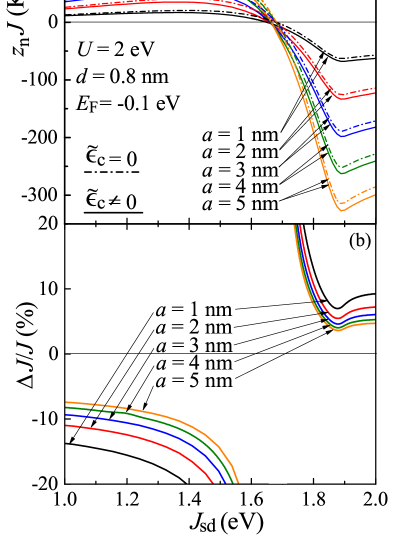
Figure 3: (Color online) (Upper panel) Exchange interaction vs grain size $a$ and spin subband splitting $\mathit{J}_{\mathrm{sd}}\in[1;2]$ eV for $d=0.8$ nm, $U=2$ eV, and $E_{\mathrm{F}}=-0.1$ eV and coordination number $z_{\mathrm{n}}=6$. (Lower panel) The relative difference of the intergrain exchange coupling $\Delta J/J$ vs spin subband splitting $\mathit{J}_{\mathrm{sd}}$ for different grain sizes $a$.

Figure 3 shows a variation of the exchange interaction between magnetic grains embedded into insulating matrix for different dielectric constants and the same barrier height. The curves are calculated using (12) and (17). The upper panel shows the intergrain exchange interaction vs spin subband splitting $\mathit{J}_{\mathrm{sd}}$ for the following parameters: barrier height $h_{\mathrm{B}}=-E_{\mathrm{F}}=0.1$ eV, $U=2$ eV, $d=0.8$ nm. Several curves are shown for different grain sizes ranging from 1 to 5 nm. Solid lines correspond to finite charging energy, $\tilde{\epsilon}_{\mathrm{c}}=0.14/a$ eV ($a$ is in nm) and $\varepsilon=5$. Dash-dotted curves correspond to infinite dielectric constant where the Coulomb blockade is negligible, $\tilde{\epsilon}_{\mathrm{c}}\approx 0$. For any grain sizes the exchange interaction has a peak in the vicinity of $\mathit{J}_{\mathrm{sd}}=0.7U$. The peak value grows with the grain size $a$. The exchange coupling is strong and exceeds 100 K for grains with radius 5 nm. Thus, transition between the SPM and SFM states in granular magnets is experimentally observable. For $J_{\mathrm{sd}}>(E_{\mathrm{F}}+U)$ the exchange interaction becomes of AFM type. The absolute value of AFM coupling reaches its maximum at $J_{\mathrm{sd}}\approx 0.9U$.

One can see that the change in the exchange interaction with changing the insulating dielectric constant is pronounced for grains with $a=5$ nm. The ordering temperature variation due to the Coulomb blockade is of the order of 10-20 K. The curves with zero charging energy $\tilde{\epsilon}_{\mathrm{c}}$ are located above the curves with finite $\tilde{\epsilon}_{\mathrm{c}}$ meaning that the third “hopping” term in the exchange interaction in (12) and (17) results in positive FM contribution. Therefore, the Coulomb blockade effects, which are pronounced for small dielectric constants $\varepsilon$ and small grains, reduce the FM coupling between the grains.

The lower panel shows the relative difference (in %) between the solid and the dash-dotted lines of the upper panel, $\Delta J/J$, calculated using (12) and (17). These curves show that the relative change of the intergrain exchange interaction due to the Coulomb interaction can be a few tens of percent. The relative change grows with decreasing the grain size meaning that the Coulomb blockade effects are more pronounced for small grains.

Figure 4 shows the relative change of the exchange interaction $\Delta J/J$ vs $U$ (or the Fermi momentum $k^{2}_{\mathrm{F}}=2m_{\mathrm{e}}(U+E_{\mathrm{F}})/\hbar^{2}$) and the spin subband splitting $\mathit{J}_{\mathrm{sd}}$. Two bright (blue and red) diagonal lines appear in the vicinity of the zero exchange. These lines divide the whole space into regions of AFM and FM coupling. The relative change of the exchange interaction $\Delta J/J$ grows sharply, reaching infinity when $J|_{\tilde{\epsilon}_{\mathrm{c}}\neq 0}+J|_{\tilde{\epsilon}_{\mathrm{c}}=0}=0$ ($J_{0}\approx 0$). This produces the red and the blue spots along the two diagonals in figure 4.

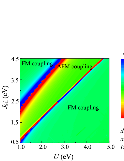
Figure 4: (Color online) Relative change of exchange interaction $\Delta J/J$ vs $U$ and spin subband splitting $\mathit{J}_{\mathrm{sd}}$ for $d=0.9$ nm, $a=3$ nm, and $E_{\mathrm{F}}=-0.1$ eV.

In general, the relative difference grows with reducing the Fermi momentum (or $U$). This can be understood as follows: The exchange interaction is the result of virtual electron hopping between the grains. The hopping is related to the kinetic energy of electrons with characteristic energy scale $E_{\mathrm{F}}$. The larger the ratio $E_{\mathrm{C}}/E_{\mathrm{F}}$ the stronger the influence of many-body effects on hopping and thus on the intergrain exchange coupling. Since the exchange interaction is stronger for large spin subband splitting ($J_{\mathrm{sd}}>(U+E_{\mathrm{F}})$) the influence of the Coulomb interaction is more pronounced in this region too.

To observe the influence of the Coulomb interaction on the exchange interaction $J$ experimentally one can either use the insulating matrix with different dielectric constants or use materials with dielectric constant being dependent on some parameter. The first approach is difficult since insulators with different dielectric constants $\varepsilon$ have different electron energy barriers. The second approach looks more promising. For example, one can use ferroelectrics with temperature or field dependent dielectric constant to control the magnetic interaction in GFM.

6.4 Exchange interaction vs grain size $a$ and the spin subband splitting $\mathit{J}_{\mathrm{sd}}$

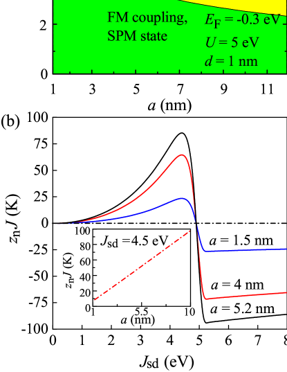
Figure 5: (Color online) (a) Magnetic phase diagram of granular magnet as a function of grain size $a$ and the spin subband splitting $\mathit{J}_{\mathrm{sd}}$ for the following parameters: $d=1$ nm, $U=5$ eV, and $E_{\mathrm{F}}=-0.1$ eV. Color shows the value of the product of intergrain coupling $J$ and coordination number $z_{\mathrm{n}}=6$. The region of SFM state ($z_{\mathrm{n}}J>T$) is shown for temperature $T=100$ K. For negative $J$ the SSG state appears at some temperature. The SPM state is shown for $|z_{\mathrm{n}}J|<T$. (b) Intergrain exchange coupling $J$ vs spin subband splitting $\mathit{J}_{\mathrm{sd}}$ for different grain sizes $a$. Inset: intergrain exchange interaction $J$ vs the grain size $a$ for $\mathit{J}_{\mathrm{sd}}=4.5$ eV.

The Coulomb blockade effect depends on the grain size $a$: the smaller the grain size the stronger the Coulomb blockade. Figure 5 shows the intergrain exchange interaction vs grain size $a$ and the spin subband splitting, $\mathit{J}_{\mathrm{sd}}$ for given intergrain distance $d=1$ nm, barrier height $h_{\mathrm{B}}=0.1$ eV and $U=5$ eV. We assume that the effective dielectric constant of the medium outside the grains is $\varepsilon=5$. This value corresponds to $a\tilde{\epsilon}_{\mathrm{c}}=0.14$ eV$\cdot$nm. Figure 5 shows that the coupling between the grains can be either FM or AFM. The dash-dotted line ($J=0$ K) in figure 5 divides the regions of FM and AFM coupling: the small spin subband splitting $\mathit{J}_{\mathrm{sd}}$ results in the FM intergrain coupling, while the strong splitting leads to the AFM exchange interaction between the grains. Transitions between the two regions occur at $J\approx(U+E_{\mathrm{F}})$.

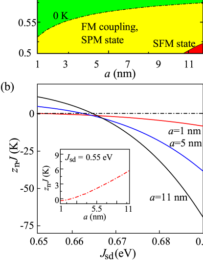
Figure 6: (Color online) (a) Magnetic phase diagram of granular magnet as a function of grain size $a$ and the spin subband splitting $\mathit{J}_{\mathrm{sd}}$ for $d=0.8$ nm, $U=1$ eV, and $E_{\mathrm{F}}=-0.1$ eV. Color shows the value of $z_{\mathrm{n}}J$. The regions of SFM ordering ($z_{\mathrm{n}}J>T$) is shown for temperature $T=20$ K. For large enough negative value of $J$ the super-spin glass state may appear. The SPM state appears at $|z_{\mathrm{n}}J|<T$. (b) Intergrain exchange coupling vs spin subband splitting $\mathit{J}_{\mathrm{sd}}$ for different grain sizes $a$. Inset: intergrain exchange coupling $J$ vs the grain size for $\mathit{J}_{\mathrm{sd}}=0.55$ eV.

For large values of Fermi momentum $k_{\mathrm{F}}$ the transition from FM to AFM coupling does not depend on the grain size ($J_{1}\ll J_{0}$). Therefore the $J=0$ K line is straight and parallel to the horizontal axis. The kinetic energy of electrons in this case exceeds the Coulomb energy reducing the role of the Coulomb blockade effects.

The long-range SFM order in granular array appears when the product $z_{\mathrm{n}}J$ reaches the system temperature $T$. This region is shown for temperature $T=100$ K. A strong AFM coupling leads to the formation of SSG state in disordered granular magnets. Inset in figure 5(b) shows the intergrain coupling vs the grain size. For high electron concentration, large $k_{\mathrm{F}}$, the dependence is linear. In this case the influence of the third “hopping” term in (12) and (17) on the intergrain exchange interaction is small and the Coulomb blockade does not influence the exchange interaction. This result corresponds to the case of grains made of strong FM metals such as Fe, Ni or Co with wide conduction band.

Note that the exchange coupling $J$ is the total interaction energy between two grains. It linearly grows with the grain size. At the same time the areal interaction energy (exchange coupling per unit surface area, or even per atom) does not grow with the grain size. Moreover, the areal exchange coupling even decreases with $a$ since the effective interaction area ($\sim a\varkappa$) is much smaller than the total grain surface ($\sim a^{2}$). This is due to spherical shape of the grains.

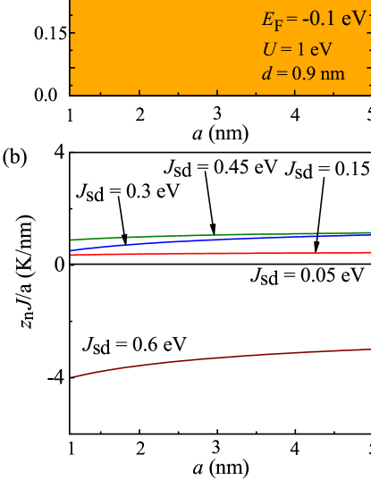
Figure 7: (Color online) (a) Magnetic phase diagram: normalized exchange interaction $z_{\mathrm{n}}J/a$ vs the grain size $a$ and the spin subband splitting $\mathit{J}_{\mathrm{sd}}$ for $d=0.9$ nm, $U=1$ eV, and $E_{\mathrm{F}}=-0.1$ eV. Color shows the value of $z_{\mathrm{n}}J/a$. (b) Normalized exchange interaction $z_{\mathrm{n}}J/a$ vs grain size $a$ for different spin subband splitting $\mathit{J}_{\mathrm{sd}}$.

Figure 6 shows the intergrain exchange coupling vs grain size $a$ and the spin subband splitting $\mathit{J}_{\mathrm{sd}}$ for a given intergrain distance $d=0.8$ nm, barrier height $h_{\mathrm{B}}=0.1$ eV, $U=1$ eV, and $a\tilde{\epsilon}_{\mathrm{c}}=0.14$ eV$\cdot$nm (small Fermi momentum and low electron concentration). For small Fermi momentum the Coulomb interaction can substantially modify the intergrain exchange coupling. In this case the curve $J=0$ K is no longer a straight line. Figure 6 shows that the exchange coupling changes its sign from FM to AFM with reducing the grain size at fixed $\mathit{J}_{\mathrm{sd}}$ (see inset in figure 6(b)).

To observe the influence of the Coulomb interaction on the exchange coupling experimentally one can measure the normalized SFM ordering temperature as a function of grain size $a$. In the absence of Coulomb blockade the exchange interaction $J$ is a linear function of $a$ and so is the ordering temperature, $T_{\mathrm{ord}}=z_{\mathrm{n}}J\sim a$. In the presence of Coulomb blockade the dependence $J(a)$ is more complicated. The ratio $T_{\mathrm{ord}}/a$ as a function of $a$ provides information about the influence of the Coulomb blockade. For zero Coulomb interaction the normalized ordering temperature is constant and does not depend on $a$. The Coulomb interaction results in deviation of $T_{\mathrm{ord}}/a$ from the straight line. Figure 7 shows the normalized exchange interaction (or ordering temperature) as a function of grain size $a$ and spin subband splitting $\mathit{J}_{\mathrm{sd}}$. Figure 7(b) shows the normalized ordering temperature as a function of $a$ for different $\mathit{J}_{\mathrm{sd}}$.

The influence of Coulomb blockade on the intergrain exchange interaction is especially pronounced in GFM made of FM metals with small Fermi momentum and large spin subband splitting. Halfmetals with low electron concentration at the Fermi level and full spin subband splitting such as CrO₂ and Sr₂FeMoO$6$ [46, 47] would be good candidates for observation of many-body effects in GFM.

7 Validity of our model

Below we discuss several assumptions and approximations of our theory.

1) In our consideration we took into account only elastic transitions of electrons and neglected the inelastic sequential tunneling between grains. At finite temperature sequential tunneling also contribute to the exchange interaction. Elastic transitions contribute to the exchange coupling only in the second order perturbation theory (in the tunneling matrix element), while sequential tunneling contributes in the first order perturbation theory. In our consideration sequential tunneling can be neglected since these transitions are exponentially suppressed due to the Coulomb blockade effects. The electron spectrum in the grains has a Coulomb gap $\tilde{\epsilon}_{\mathrm{c}}$ leading to the exponential suppression of inelastic sequential tunneling, $\rme^{-\tilde{\epsilon}_{\mathrm{c}}/T}$. Elastic processes are also suppressed due to the gap but only algebraically, $1/\tilde{\epsilon}_{\mathrm{c}}$. Similar situation exists in granular metals [15]: Elastic co-tunneling, appearing in the second or higher order perturbation theory, exceeds at low temperatures the inelastic sequential tunneling appearing in the first order perturbation theory.

2) We discussed the influence of the diagonal spin-independent part of the Coulomb interaction on the intergrain exchange coupling and neglected the spin-dependent part of the Coulomb interaction between electrons located at different grains. However, the overlap of electron wave functions in the insulator between the grains produces finite spin dependent matrix elements of the Coulomb interaction, which originally was called the exchange coupling [48]

$$U^{\mathrm{ex}}_{ijkl}=\!\int\!\!\int d^{3}\bi r_{1}d^{3}\bi r_{2}\psi^{*}_{i}(\bi r_{1})\phi_{l}(\bi r_{1})\hat{U}_{\mathrm{C}}\psi_{j}(\bi r_{2})\phi^{*}_{k}(\bi r_{2}),$$ (24)

where $\hat{U}_{\mathrm{C}}$ is the Coulomb interaction operator. This term requires a separate consideration.

3) We assumed the parabolic electron spectrum in our model. In our theory the hopping based exchange interaction can be either AFM or FM depending on the shift of the spin subband. Taking into account the real band structure via ab initio modeling will provide an additional insight into the problem, however it requires more complicated calculations. The ab initio calculations of band structure of FM metals can be used to estimate the effective parameters in the Hamiltonian in (1). Also these parameters can be estimated using spectroscopic experiments and experiments on tunneling magneto-resistance in magnetic tunnel junctions.

4) We note that the theory developed in this paper fails as the intergrain distance tends to zero. Decrease in intergrain distance leads to the increase in tunneling probability. At some point the approximation of wave functions localized at different grains is not valid. In this case the better starting point is to use the wave functions delocalized on the scale of the whole granular magnet.

8 Conclusion

We developed a theory of the exchange interaction between FM metallic grains embedded into insulating matrix by taking into account many-body effects. In particular, we considered the Coulomb blockade effects. These effects can be neglected for layered structures, however they are crucial for nanogranular systems. For bulk ferromagnets separated by the insulating layer the exchange interaction depends on the barrier height for electrons inside the insulator. We showed that due to the Coulomb blockade effects the exchange coupling between FM grains embedded into insulating matrix additionally depends on the dielectric properties of this matrix. In particular, the FM coupling decreases with decreasing the dielectric permittivity of insulator. The Coulomb blockade effects prevent virtual transitions of electrons between the grains and shift the intergrain coupling toward the AFM type. We showed that the variation in the exchange interaction due to the Coulomb blockade effects can be a few tens of percent.

We studied the behavior of intergrain exchange interaction $J$ as a function of grain size $a$. We showed that there are two factors defining this behavior: 1) The geometrical factor - the increase in the grain size leads to the increase in the interaction strength. We find that in contrast to layered structure, where exchange interaction grows linearly with the surface area of the system, $J\sim a^{2}$, in granular system the exchange coupling depends linearly on the grain size, $J\sim a$. 2) The influence of grain size on the Coulomb blockade effects and thus on the intergrain exchange interaction. The smaller the grain the larger the Coulomb blockade the smaller the FM contribution to the exchange interaction. We found that the exchange interaction decays faster than the first power of $a$ with decreasing the grain size and showed that the transition from the FM to AFM coupling exists with decreasing the grain size.

The Coulomb blockade effects are important if charging energy essentially exceeds the characteristic energy interval contributing to the exchange interaction. This interval depends on the barrier height of the insulator and barrier thickness. The influence of Coulomb blockade effects is more pronounced for thick and low barrier. We investigated the intergrain exchange coupling as a function of system parameters such as internal subband splitting and the Fermi energy. The Coulomb blockade influences the intergrain exchange coupling strongly if: 1) the Fermi momentum is not too large and 2) the spin subband splitting is of the order of the Fermi energy.

9 Acknowledgements

This research was supported by NSF under Cooperative Agreement Award EEC-1160504, the U.S. Civilian Research and Development Foundation (CRDF Global) and NSF PREM Award. O.U. was supported by Russian Science Foundation (Grant 16-12-10340).

Appendix A Single grain wave functions

Consider single spherical metallic grain with radius $a$. The orbital part of the electron wave function in a state with orbital quantum numbers ($mln$) and a spin state $s$ has the form

$$\psi^{s}_{mln}=R^{s}_{nl}(r)Y_{ml}(\varphi,\theta),$$ (25)

where $Y_{ml}(\varphi,\theta)$ is the spherical function and $R^{s}_{nl}(r)$ is governed by the equation

$$\frac{1}{r^{2}}\frac{\partial}{\partial r}\left(r^{2}\frac{\partial R^{s}_{nl}}{\partial r}\right)-\frac{l(l+1)R^{s}_{nl}}{r^{2}}+\frac{2m_{\mathrm{e}}}{\hbar^{2}}(E^{s}_{n}-\hat{U}_{\mathrm{sp}})R^{s}_{nl}=0.$$ (26)

Here $U_{\mathrm{sp}}$ stands for $s$ component of either $\hat{U}_{1}+\hat{H}_{1\mathrm{m}}$ or $\hat{U}_{2}+\hat{H}_{2\mathrm{m}}$ depending on the grain. The largest contribution to the intergrain exchange interaction appears due to electrons in the vicinity of the Fermi surface. Using the quasiclassical approximation [48] for these electrons outside the metallic grain we find

$$\eqalign{R^{s}_{nl}(r)=\frac{C\hbar}{r\left(2m_{\mathrm{e}}\left(\frac{\hbar^{2}l(l+1)}{2m_{\mathrm{e}}r^{2}}-E^{s}_{n}\right)\right)^{1/4}}\times\cr\times\exp\left(-\frac{1}{\hbar}\int_{a}^{r}\sqrt{2m_{\mathrm{e}}\left(\frac{\hbar^{2}l(l+1)}{2m_{\mathrm{e}}r^{2}}-E^{s}_{n}\right)}dr\right),}$$ (27)

where $E^{s}_{n}$ stands for the total energy of electron in the radial state $n$ and the spin state $s$. We assume that the grain size $a$ is larger than the distance between the grains surfaces $d$. Therefore we will neglect the dependence of the effective potential on $r$ in between the grains

$$\eqalign{R^{s}_{nl}(r)=\frac{C\hbar}{r\left(2m_{\mathrm{e}}\left(\frac{\hbar^{2}l(l+1)}{2m_{\mathrm{e}}a^{2}}-E^{s}_{n}\right)\right)^{1/4}}\times\cr\times\exp\left(-\frac{1}{\hbar}(r-a)\sqrt{2m_{\mathrm{e}}\left(\frac{\hbar^{2}l(l+1)}{2m_{\mathrm{e}}a^{2}}-E^{s}_{n}\right)}\right).}$$ (28)

For the left grain wave function $\psi$ we introduce $r=\sqrt{r_{\perp}^{2}+(a+d/2+z)^{2}}$ and for the right grain wave function $\phi$ we introduce $r^{\prime}=\sqrt{r_{\perp}^{2}+(a+d/2-z)^{2}}$. We use the notation $\varkappa^{s}_{nl}=-\frac{1}{\hbar}\sqrt{2m_{\mathrm{e}}\left(\frac{\hbar^{2}l(l+1)}{2m_{\mathrm{e}}a^{2}}-E^{s}_{n}\right)}$. For small $r_{\perp}$ we find

$$R^{s}_{nl}(z,r_{\perp})\approx\frac{C}{a\sqrt{\varkappa^{s}_{nl}}}\exp\left(-\varkappa^{s}_{nl}\left(\frac{d}{2}\pm z+\frac{r_{\perp}^{2}}{2a}\right)\right),$$ (29)

where the sign $\pm$ corresponds to the wave function of the left and right grains and $C$ is the normalization constant.

Inside the grain the wave function consists of two waves propagating outward and toward the particle centre.

$$R^{s}_{nl}(z,r_{\perp}\!)\!\approx\!\!\frac{C_{\mathrm{i}}}{a\sqrt{k^{s}_{nl}}}\!\!\left(\rme^{\rmi k_{nl}^{s}\left(\!\!\frac{d}{2}\pm z+\frac{r_{\perp}^{2}}{2a}\right)}\!\!\!+\xi^{s}_{nl}\rme^{-\rmi k^{s}_{nl}\left(\!\!\frac{d}{2}\pm z+\frac{r_{\perp}^{2}}{2a}\right)}\!\!\right)\!\!.$$ (30)

Here $\xi^{s}_{nl}=\frac{k_{nl}^{s}-\rmi\varkappa^{s}_{nl}}{k_{nl}^{s}+\rmi\varkappa^{s}_{nl}}$ is the amplitude of the reflected electron wave, $k^{s}_{nl}=-\frac{1}{\hbar}\sqrt{2m_{\mathrm{e}}\left(U-s\mathit{J}_{\mathrm{sd}}+\frac{\hbar^{2}l(l+1)}{2m_{\mathrm{e}}a^{2}}-E^{s}_{n}\right)}$, and $C_{\mathrm{i}}$ is the normalization constant. Below we will use the symbols $i$ and $j$ to describe a set of quantum numbers characterizing the orbital motion of electrons. The overlap of wave functions of electrons $i$ and $j$ located in different grains exists only between the grains in a small region in the vicinity of $r_{\perp}=0$. The in-plane area (($x,y$)-plane) of the overlap region is $S^{ij}_{\mathrm{c}}=\pi(\lambda^{ij}_{\perp})^{2}$, where $\lambda^{ij}_{\perp}=\sqrt{2a/(\varkappa_{i}+\varkappa_{j})}$. For electrons at the Fermi level we introduce the size $\lambda_{\perp}=\sqrt{a/\varkappa_{0}}$ and the corresponding area $S_{\mathrm{c}}=\pi\lambda^{2}_{\perp}$.  This estimate for overlap region works for $d\ll a$ and $S_{\mathrm{c}}\ll\pi a^{2}$.

To further simplify the wave function we change the spherical wave with the plane one. The wave function magnitude in (29) exponentially decays in the ($x,y$) plane. We change it with the wave function having constant magnitude in the region $r_{\perp}<\sqrt{2a/\varkappa}$. This is schematically shown in figure 8. Instead of factor $\rme^{-\varkappa r_{\perp}^{2}/(2a)}$ we put 1 in the region $r_{\perp}<\sqrt{2a/\varkappa}$ and 0 outside the region. Generally, one can use numerical calculations to avoid this simplification.

Figure 8: (Color online) Wave function magnitude vs $r_{\perp}$. Red line shows the wave function given by (29). Blue line shows the model wave function used in the calculation of the matrix elements.

The important difference with the case of infinite semispaces is related to the fact that the interaction between electrons at different grains occurs only in the small area $S^{ij}_{\mathrm{c}}$. This area is small in comparison with the grain surface and grows linearly with the grain size $a$ (instead of $a^{2}$). This geometric factor decreases the interaction between the grains.

The size of the interaction region is much larger than the Fermi length of electrons in metallic grains. Therefore we can change quantum numbers ($mln$) to $(k_{x}k_{y}k_{z})$. Introducing $k_{\perp}=\sqrt{k^{2}_{x}+k^{2}_{y}}\approx l/a$ and the total electron energy, $E^{s}k=U+s\mathit{J}_{\mathrm{sd}}+\hbar^{2}(k^{2}_{\perp}+k_{z}^{2})/(2m_{\mathrm{e}})$ we obtain the electron wave functions outside and inside the grains in (6) and (7).

Appendix B Matrix elements

B.1 FM ordering

Using (6) and (7) we find for matrix elements the following results

$$\eqalign{V^{s}_{ii}=\int_{-\tilde{\lambda}_{\perp}}^{\tilde{\lambda}_{\perp}}dxdy\int_{d/2}^{\infty}dz|\psi^{s}_{i}|^{2}(-U+s\mathit{J}_{\mathrm{sd}})=\cr=(s\!\mathit{J}_{\mathrm{sd}}-U)\frac{(|\tau^{s}_{i}|)^{2}}{2\Omega\varkappa_{i}^{s}}\rme^{-2\varkappa_{i}^{s}d}F_{1}(q),\cr P_{ij}^{s}=\int_{-\tilde{\lambda}_{\perp}}^{\tilde{\lambda}_{\perp}}dxdy\int_{-\infty}^{\infty}dz\phi^{s*}_{i}\psi^{s}_{j}=\frac{T_{ij}^{s}+T_{ji}^{s*}}{s\!\mathit{J}_{\mathrm{sd}}-U}+\cr+\frac{\tau^{s*}_{i}\tau^{s}_{j}\rme^{-(\!\varkappa^{s}_{i}+\varkappa^{s}_{j}\!)\frac{d}{2}}\mathrm{sinh}(\!(\!\varkappa^{s}_{i}-\varkappa^{s}_{j}\!)\frac{d}{2})}{\Omega(\varkappa_{i}^{s}-\varkappa^{s}_{j})}F_{2}(q),\cr T^{s}_{ij}=\int_{-\tilde{\lambda}_{\perp}}^{\tilde{\lambda}_{\perp}}dxdy\int_{d/2}^{\infty}dz\phi^{s*}_{i}\psi^{s}_{j}(-U+s\mathit{J}_{\mathrm{sd}})=\cr=(s\!\mathit{J}_{\mathrm{sd}}-U)\frac{\tau^{s*}_{i}\tau^{s}_{j}(\varkappa_{i}^{s}+\varkappa_{j}^{s})}{\Omega((k_{i}^{s})^{2}+(\varkappa_{j}^{s})^{2})}\rme^{-\varkappa_{j}^{s}d}F_{3}(q).}$$ (31)

The wave functions are overlapped in a finite area in the (x,y)-plane and therefore $k_{x}$ and $k_{y}$ components of electron momentum do not conserve during the transitions. To calculate matrix elements $V_{ii}^{s}$, $P_{ij}^{s}$ and $T_{ij}^{s}$ we approximate the wave functions in (6) and (7) with plane waves confined within a square window in the perpendicular direction. The size of this window is defined by the suppression factor $\rme^{-\varkappa r^{2}_{\perp}/2a}$ in the expression for the wave functions. We change this factor with a step function being finite in a square $|x|<\tilde{\lambda}_{\perp}$, $|y|<\tilde{\lambda}_{\perp}$ and zero outside this region. Therefore, instead of circular integral region we consider the rectangular region. Integrals of the type $\int_{|x|<\lambda_{\perp}}\rme^{-\rmi q_{x}x}\sim\mathrm{Sinc}(q\lambda_{\perp})$ produce $\mathrm{Sinc}$-like factors in the matrix elements. The size of $\tilde{\lambda}_{\perp}$ is different for different matrix elements and is defined by the wave functions overlap area. For matrix elements $V^{s}_{ii}$ the size of the overlap area is $\lambda_{\perp}^{2}=\pi a/\varkappa_{i}$, for the tunneling matrix elements $T^{s}_{ij}$ the size is $\lambda_{\perp}^{2}=2\pi a/\varkappa_{j}$. The overlap term $P^{s}_{ij}$ has three contributions: The first two have the same area as $T^{s}_{ij}$ and the last contribution has the area $\lambda_{\perp}^{2}=2\pi a/(\varkappa_{i}+\varkappa_{j})$. Using these approximations we have the following result for functions $F_{i}$ in (31)

$$\eqalign{F_{1}=\frac{\pi a}{\varkappa^{s}_{i}}\mathrm{sinc}\left(\frac{q_{x}}{2}\sqrt{\frac{\pi a}{\varkappa^{s}_{i}}}\right)\mathrm{sinc}\left(\frac{q_{y}}{2}\sqrt{\frac{\pi a}{\varkappa^{s}_{i}}}\right),\cr F_{2}=\frac{2\pi a}{\varkappa^{s}_{i}+\varkappa^{s}_{j}}\mathrm{sinc}\!\!\left(\frac{q_{x}}{2}\sqrt{\frac{2\pi a}{\varkappa^{s}_{i}+\varkappa^{s}_{j}}}\right)\!\!\mathrm{sinc}\!\!\left(\frac{q_{y}}{2}\sqrt{\frac{2\pi a}{\varkappa^{s}_{i}+\varkappa^{s}_{j}}}\right),\cr F_{3}=\frac{2\pi a}{\varkappa^{s}_{j}}\mathrm{sinc}\left(\frac{q_{x}}{2}\sqrt{\frac{2\pi a}{\varkappa^{s}_{j}}}\right)\mathrm{sinc}\left(\frac{q_{y}}{2}\sqrt{\frac{2\pi a}{\varkappa^{s}_{j}}}\right),}$$ (32)

where $\bi q=\bi k_{i\perp}-\bi k_{j\perp}$, $k_{i\perp}=(k_{ix},k_{iy},0)$ and $q=|\bi q|$. Factors $F_{1,2,3}$ decay rapidly outside the region $|q|>1/\lambda_{\perp}$.

B.2 AFM ordering

For AFM ordering the grain magnetic moments are anti-parallel. The superscripts in all matrix elements refer to the spin state in the first grain. The spin state in the second grain is the opposite to the spin state in the first grain. Using the same approach as above for matrix elements we find

$$\eqalign{V^{s}_{ii}=(-s\!\mathit{J}_{\mathrm{sd}}-U)\frac{(|\tau^{s}_{i}|)^{2}}{2\Omega(\varkappa_{i}^{s})}\rme^{-2\varkappa_{i}^{s}d}F_{1}(q),\cr T^{s}_{ij}\!=(-s\!\mathit{J}_{\mathrm{sd}}-U)\frac{\tau^{-s*}_{i}\tau^{s}_{j}(\varkappa_{i}^{-s}\!\!+\varkappa_{j}^{s})}{\Omega(\!(k_{i}^{-s})^{2}+\!(\varkappa_{j}^{s})^{2})}\rme^{-\varkappa_{j}^{s}\!d}F_{3}(q),\cr P_{ij}^{s}=\frac{T_{ji}^{-s*}}{s\!\mathit{J}_{\mathrm{sd}}-U}+\frac{T_{ij}^{s}}{-s\!\mathit{J}_{\mathrm{sd}}-U}+\\ +\frac{\tau^{-s*}_{i}\tau^{s}_{j}\rme^{-(\!\varkappa^{-s}_{i}+\varkappa^{s}_{j}\!)\frac{d}{2}}\mathrm{sinh}(\!(\!\varkappa_{i}^{-s}-\varkappa_{j}^{s}\!)\frac{d}{2})}{\Omega((\varkappa_{i}^{-s})-(\varkappa_{j}^{s}))}F_{4}(q),}$$ (33)

where

$$F_{4}=\frac{2\pi a}{\varkappa^{-s}_{i}\!\!+\!\varkappa^{s}_{j}}\mathrm{sinc}\!\!\left(\!\frac{q_{x}}{2}\sqrt{\frac{2\pi a}{\varkappa^{-s}_{i}\!\!+\!\varkappa^{s}_{j}}}\right)\!\!\mathrm{sinc}\!\!\left(\!\frac{q_{y}}{2}\sqrt{\frac{2\pi a}{\varkappa^{-s}_{i}\!\!+\!\varkappa^{s}_{j}}}\right)\!.$$ (34)

Appendix C Formalism

Here we consider only the case of FM ordering of grains magnetic moments. The case of AFM ordering can be considered in a similar way. The zero order wave function is the Slater determinant

$$\Psi_{0}=\frac{1}{\sqrt{N}}\left(\eqalign{\psi^{s_{1}}_{1}(\bi r_{1})~{}~{}~{}...~{}~{}~{}\psi^{s_{1}}_{1}(\bi r_{2n_{0}})\cr~{}~{}~{}~{}~{}~{}~{}~{}~{}~{}~{}~{}~{}...\cr\phi^{s_{n_{0}+1}}_{1}(\bi r_{1})~{}...~{}\phi^{s_{n_{0}+1}}_{1}(\bi r_{2n_{0}})\cr~{}~{}~{}~{}~{}~{}~{}~{}~{}~{}~{}~{}~{}...}\right).$$ (35)

States $\psi_{i}$ and $\phi_{j}$ are chosen such that all the energy levels below $E_{\mathrm{F}}$ are filled: $n_{0}$ states in the left grain and $n_{0}$ states in the right grain. The normalizing factor is

$$N=(2n_{0})!(1-2\sum_{i,j,s}|P_{ij}^{s}|^{2}+...),$$ (36)

where $i$ and $j$ enumerate states in the left and the right grains, respectively. The second term in (36) appears due to nonorthogonality of the basis wave functions. Further we introduce the excited states as follows

$$\Psi_{ij}^{s}=\hat{b}^{s+}_{i}\hat{a}^{s}_{j}\Psi_{0}=\frac{1}{\sqrt{N_{ij}}}\left(\eqalign{\psi^{s_{1}}_{1}(\bi r_{1})~{}~{}~{}~{}~{}...~{}~{}~{}~{}~{}\psi^{s_{1}}(\bi r_{2n_{0}})\cr~{}~{}~{}~{}~{}~{}~{}~{}~{}~{}~{}~{}~{}~{}...\cr\phi^{s_{n_{0}+j-1}}_{j-1}(\bi r_{1})~{}...~{}\phi^{s_{n_{0}+j-1}}_{j-1}(\bi r_{2n_{0}})\cr\psi^{s}_{i}(\bi r_{1})~{}~{}~{}~{}~{}~{}...~{}~{}~{}~{}~{}~{}\psi^{s}_{i}(\bi r_{2n_{0}})\cr\phi^{s_{n_{0}+j+1}}_{j+1}(\bi r_{1})~{}...~{}\phi^{s_{n_{0}+j+1}}_{j+1}(\bi r_{2n_{0}})\cr~{}~{}~{}~{}~{}~{}~{}~{}~{}~{}~{}~{}~{}~{}...}\right).$$ (37)

The annihilation operator removes a line in the Slater determinant while the creation operator adds a line. The normalization factor has the form $N_{ij}=(2n_{0})!(1-2\sum_{k,l,s}|P_{kl}^{s}|^{2}+2\sum_{k,s}(2\sum_{k,s}(|P_{kj}^{s}|^{2}+|P_{jk}^{s}|^{2})-2\sum_{k,s}(2\sum_{k,s}(|P_{ki}^{s}|^{2}+|P_{ik}^{s}|^{2})...)$. One can introduce the excited wave function $\tilde{\Psi}^{s}_{ij}=\hat{a}^{s+}_{i}\hat{b}^{s}\Psi_{0}$. These wave functions correspond to single excitations with only one electron transferred between grains. The Coulomb energy of excited states is $\tilde{\epsilon}_{\mathrm{c}}$. In our calculations we neglect states with two electrons transferred between grains. Such states have large Coulomb energy, $2\tilde{\epsilon}_{\mathrm{c}}$ and therefore transitions to these states have much lower probability. Also we neglect electron transitions between the single particle states within the same grain ($\psi_{i}\to\psi_{j}$). The probability of such transitions is of order $p^{2}$. Therefore, these transitions contribute to the system energy on the level of $p^{4}$ which is beyond our accuracy ($p^{2}$). Using the above excited states we can write the perturbed wave function in (9).

To find the coefficients $\beta^{s}_{ij}$ and $\tilde{\beta}^{s}_{ij}$ in (9) we solve the Schrodinger equation

$$(\hat{H}_{\mathrm{sp}}+\hat{H}_{\mathrm{C}}-E)|(1+\alpha_{0})\Psi_{0}+\!\!\!\sum_{s,i,j}\beta_{ij}^{s}\Psi^{s}_{ij}+\!\!\!\sum_{s,i,j}\tilde{\beta}_{ij}^{s}\tilde{\Psi}^{s}_{ij}\rangle=0.$$ (38)

Selecting terms of order of $p$ we find

$$\beta^{s}_{ij}=\tilde{\beta}^{s}_{ij}=-\frac{\langle\Psi^{s}_{ij}|(\hat{H}_{\mathrm{sp}}+\hat{H}_{\mathrm{C}}-E)|\Psi_{0}\rangle}{\langle\Psi^{s}_{ij}|(\hat{H}_{\mathrm{sp}}+\hat{H}_{\mathrm{C}}-E)|\Psi^{s}_{ij}\rangle}.$$ (39)

We neglect electron transitions between the grains due to the Coulomb interaction, $\langle\Psi^{s}_{ij}|\hat{H}_{\mathrm{C}}|\Psi_{0}\rangle=0$. Using (35) and (37) we find

$$\langle\Psi^{s}_{ij}|\hat{H}_{\mathrm{sp}}|\Psi_{0}\rangle=T^{s}_{ij}+E_{0}P^{s}_{ij}\sim p,$$ (40)

where $E_{0}=2\sum_{i,s}\epsilon_{i}^{s}$ (the summation is over states below the Fermi energy). Finally we obtain

$$\langle\Psi^{s}_{ij}|(\hat{H}_{\mathrm{sp}}-E)|\Psi_{0}\rangle=T^{s}_{ij},$$ (41)

here we take into account the fact that the total energy is $E=E_{0}+O(p^{2})$. The denominator in (39) is given by the expression

$$\langle\Psi^{s}_{ij}|\hat{H}_{\mathrm{sp}}|\Psi_{ij}^{s}\rangle=\epsilon^{s}_{i}-\epsilon^{s}_{j}+\tilde{\epsilon}_{\mathrm{c}}.$$ (42)

Using (41) and (42) we obtain (10) in the main text.

To find the coefficient $\alpha_{0}$ in (9) we use the fact that the total number of electrons in the system is conserved. Introducing the operator of the total number of electrons, $\hat{N}=\sum_{i,s}\hat{a}^{s+}_{i}\hat{a}^{s}_{i}+\sum_{i,s}\hat{b}^{s+}_{i}\hat{b}^{s}_{i}$ we have the following relation

$$\eqalign{1=\frac{\langle\Psi|\hat{N}|\Psi\rangle}{N_{0}}=(1+2\alpha_{0})-4\!\!\!\!\!\!\!\!\!\sum_{s,i\notin S_{0}^{s},j\in S_{0}^{s}}\!\!\frac{\mathrm{Re}(T^{s}_{ij}P^{s*}_{ij})}{\epsilon_{i}^{s}-\epsilon_{j}^{s}+\tilde{\epsilon}_{\mathrm{c}}}+\cr+2\!\!\!\!\!\!\!\!\!\sum_{s,i\notin S_{0}^{s},j\in S_{0}^{s}}\!\!\frac{|T^{s}_{ij}|^{2}}{(\epsilon_{i}^{s}-\epsilon_{j}^{s}+\tilde{\epsilon}_{\mathrm{c}})^{2}}.}$$ (43)

Now we can calculate the system energy

$$\eqalign{E^{\mathrm{FM}}=\langle\Psi|\hat{H}_{\mathrm{sp}}+\hat{H}_{\mathrm{C}}|\Psi\rangle=(1+2\alpha_{0})\langle\Psi_{0}|\hat{H}_{\mathrm{sp}}+\hat{H}_{\mathrm{C}}|\Psi_{0}\rangle+\cr+4\sum_{i,j,s}\mathrm{Re}\left(\beta^{s*}_{ij}\langle\Psi^{s}_{ij}|\hat{H}_{\mathrm{sp}}+\hat{H}_{\mathrm{C}}|\Psi_{0}\rangle\right)+\cr+2\sum_{i,j,s}\mathrm{Re}\left(|\beta^{s}_{ij}|^{2}\langle\Psi^{s}_{ij}|\hat{H}_{\mathrm{sp}}+\hat{H}_{\mathrm{C}}|\Psi^{s}_{ij}\rangle\right).}$$ (44)

When calculating the first term, $\langle\Psi_{0}|\hat{H}_{\mathrm{sp}}+\hat{H}_{\mathrm{C}}|\Psi_{0}\rangle$, the corrections of the order of $p^{2}$ in the normalization factor $N$ should be taken into account. We obtain the following formula for the energy of the FM state

$$\eqalign{E^{\mathrm{FM}}=2\!\!\!\sum_{s,i\in S_{0}^{s}}(\epsilon_{i}^{s}+V^{s}_{ii})-2\!\!\!\!\!\sum_{s,i\in S_{0}^{s},j\in S_{0}^{s}}\mathrm{R}e(T^{s}_{ij}P^{s*}_{ij})-\cr-2\!\!\!\!\!\!\!\!\!\sum_{s,i\notin S_{0}^{s},j\in S_{0}^{s}}\frac{|T^{s}_{ij}|^{2}}{\epsilon^{s}_{i}-\epsilon^{s}_{j}+\tilde{\epsilon}_{\mathrm{c}}}.}$$ (45)

We use the fact that the mean energy level spacing is much smaller than the Fermi energy and replace the summation with integration in (45). We introduce momentum $\bi k$ instead of orbital numbers $i$ and replace the integration over the $\bi k_{1,2\perp}$ with integration over the $\bi q=\bi k_{1\perp}-\bi k_{2\perp}$ and $\tilde{\bi k}=(1/2)(\bi k_{1\perp}+\bi k_{2\perp})$. In general the boundaries of integration in these new coordinates are rather complicated. However, as we showed in the previous section all matrix elements depend only on $\bi q$ and not on $\tilde{\bi k}$. In addition, all matrix elements are finite only in the small region, $|\bi q|<\pi/\lambda_{\perp}$. Thus, we can integrate over $\bi q$ independently of $\tilde{\bi k}$ in the whole $\bi k_{\perp}$-space. Taking this into account we obtain (12) describing the energy of the FM state. The case of AFM configuration of $\bi M_{1}$ and $\bi M_{2}$ can be considered in a similar way.

References

References

- [1] Bhaskar Das, Balamurugan Balasubramanian, Priyanka Manchanda, Pinaki Mukherjee, Ralph Skomski, George C. Hadjipanayis, and David J. Sellmyer. Nano Lett., 16:1132, 2016.
- [2] Jose A. DeToro, Daniel P. Marques, Pablo Muniz, Vassil Skumryev, Jordi Sort, Dominique Givord, and Josep Nogues. Phys. Rev. Lett., 115:057201, 2015.
- [3] Ana Balan, Peter M. Derlet, Arantxa Fraile Rodriguez, Joachim Bansmann, Rocio Yanes, Ulrich Nowak, Armin Kleibert, and Frithjof Nolting. Phys. Rev. Lett., 112:107201, 2014.
- [4] Hao-Bo Li, Mengyin Liu, Feng Lu, Weichao Wang, Yahui Cheng, Shutao Song, Yan Zhang, Zhiqing Li, Jie He, Hui Liu, Xiwen Du, and Rongkun Zheng. Appl. Phys. Lett., 106:012401, 2015.
- [5] C-H. Lambert, S. Mangin, B. S. D. Ch. S. Varaprasad, Y. K. Takahashi, M. Hehn, M. Cinchetti, G. Malinowski, K. Hono, Y. Fainman, M. Aeschlimann, and E. E. Fullerton. Science, 345:1337, 2014.
- [6] D. Bartov, A. Segal, M. Karpovski, and A. Gerber. Phys. Rev. B, 90:144423, 2014.
- [7] Hyungsuk K. D. Kim, Laura T. Schelhas, Scott Keller, Joshua L. Hockel, Sarah H. Tolbert, and Gregory P. Carman. Nano Lett., 13:884, 2013.
- [8] M Woinska, J Szczytko, A Majhofer, J Gosk, K Dziatkowski, and A Twardowski. Phys. Rev. B, 88:144421, 2013.
- [9] V. I. Belotelov, I. A. Akimov, M. Pohl, V. A. Kotov, S. Kasture, A. S. Vengurlekar, Achanta Venu Gopal, D. R. Yakovlev, A. K. Zvezdin, and M. Bayer. Nature Nanotechnology, 6:370, 2011.
- [10] A D Liu and H N Bertram. J. Appl. Phys., 89:2861, 2001.
- [11] O G Udalov, N M Chtchelkatchev, and I S Beloborodov. Phys. Rev. B, 89:174203, 2014.
- [12] O G Udalov, N M Chtchelkatchev, and I S Beloborodov. J. Phys.: Condens. Matter, 27:186001, 2015.
- [13] O G Udalov, N M Chtchelkatchev, and I S Beloborodov. Phys. Rev. B, 92:045406, 2015.
- [14] A M Belemuk, O G Udalov, N M Chtchelkatchev, and I S Beloborodov. J. Phys.: Condens. Matter, 28:126001, 2016.
- [15] I S Beloborodov, A V Lopatin, V M Vinokur, and K B Efetov. Rev. Mod. Phys., 79:469, 2007.
- [16] Y. Shapira and G. Deutscher. Phys. Rev. B, 27:4463, 1983.
- [17] N. Hadacek, M. Sanquer, and J. C. Villegier. Phys. Rev. B, 69:024505, 2004.
- [18] B. S. Skrzynski, I. S. Beloborodov, and K. B. Efetov. Phys. Rev. B, 65:094516, 2002.
- [19] O G Udalov, N M Chtchelkatchev, A Glatz, and I S Beloborodov. Phys. Rev. B, 89:054203, 2014.
- [20] O G Udalov, N M Chtchelkatchev, and I S Beloborodov. Phys. Rev. B, 90:054201, 2014.
- [21] O G Udalov, A Glatz, and I S Beloborodov. Euro. Phys. Lett., 104:47004, 2013.
- [22] George C. Hadjipanayis. Jornal of Magnetism and Magnetic Materials, 200:373, 1999.
- [23] S. Ohnuma, M. Ohnuma, H. Fujimori, and T. Masumoto. Jornal of Magnetism and Magnetic Materials, 310:2503, 2007.
- [24] Hiroyasu Fujimori, Shigehiro Ohnuma, Nobukiyo Kobayashi, and Tsuyosi Masumoto. Jornal of Magnetism and Magnetic Materials, 304:32, 2006.
- [25] G Ayton, M J P Gingras, and G N Patey. Phys. Rev. Lett., 75:2360, 1995.
- [26] S Ravichandran and B Bagchi. Phys. Rev. Lett., 76:644, 1996.
- [27] C Djurberg, P Svedlindh, P Nordblad, M F Hansen, F Bodker, and S Morup. Phys. Rev. Lett., 79:5154, 1997.
- [28] S Sahoo, O Petracic, W Kleemann, P Nordblad, S Cardoso, and P P Freitas. Phys. Rev. B, 67:214422, 2003.
- [29] W Kleemann, O Petracic, C Binek, G N Kakazei, Yu G Pogorelov, J B Sousa, S Cardoso, and P P Freitas. Phys. Rev. B, 63:134423, 2001.
- [30] A A Timopheev, I Bdikin, A F Lozenko, O V Stognei, A V Sitnikov, A V Los, and N A Sobolev. J. Appl. Phys., 111:123915, 2012.
- [31] M R Scheinfein, K E Schmidt, K R Heim, and G G Hembree. Phys. Rev. Lett., 76:1541, 1996.
- [32] V N Kondratyev and H O Lutz. Phys. Rev. Lett., 81:4508, 1998.
- [33] S Bedanta, T Eimuller, W Kleemann, J Rhensius, F Stromberg, E Amaladass, S Cardoso, and P P Freitas. Phys. Rev. Lett., 98:176601, 2007.
- [34] S H Liou and C L Chien. J. Appl. Phys., 63:4240, 1988.
- [35] C L Chien. J. Appl. Phys., 69:5267, 1991.
- [36] D Kechrakos and K N Trohidou. Phys. Rev. B, 58:12169, 1998.
- [37] M El-Hilo, R W Chantrell, and K O’Grady. J. Appl. Phys., 84:5114, 1998.
- [38] U Wiedwald, M Cerchez, M Farle, K Fauth, G Schutz, K Zurn, H-G Boyen, and P Ziemann. Phys. Rev. B, 70:214412, 2004.
- [39] J C Slonczewski. Phys. Rev. B, 39:6995, 1989.
- [40] P Bruno. Phys. Rev. B, 52:411, 1995.
- [41] I S Beloborodov, A Glatz, and V M Vinokur. Phys. Rev. Lett., 99:066602, 2007.
- [42] Wenhao Wu and P. W. Adams. Phys. Rev. B, 50:13065, 1994.
- [43] I. L. Aleiner, P. W. Brouwer, and L. I. Glazman. Phys. Rep., 358:309, 2002.
- [44] H Mamiya, I Nakatani, and T Furubayashi. Phys. Rev. Lett., 82:4332, 1999.
- [45] A A Timopheev, S M Ryabchenko, V M Kalita, A F Lozenko, P A Trotsenko, V A Stephanovich, A M Grishin, and M Munakata. J. Appl. Phys., 105:083905, 2009.
- [46] Karlheinz Schwarzt. J. Phys. F: Met. Phys., 16:L211, 1986.
- [47] K.-I. Kobayashi, T. Kimura, H. Sawada, K. Terakura, and Y. Tokura. Nature, 395:677, 1998.
- [48] L D Landau and E M Lifshitz. Quantum Mechanics Nonrelativistic Theory, Course of Theoretical Physics, volume 3. Nauka, Moscow, 3 edition, 1976.