Uncovering the relation of a scalar resonance to the Higgs boson

Abstract

We consider the associated production of a scalar resonance with the standard model Higgs boson. We demonstrate via a realistic phenomenological analysis that couplings of such a resonance to the Higgs boson can be constrained in a meaningful way in future runs of the LHC, providing insights on its origin and its relation to the electroweak symmetry breaking sector. Moreover, the final state can provide a direct way to determine whether the new resonance is produced predominantly in gluon fusion or quark-anti-quark annihilation. The analysis focusses on a resonance coming from a scalar field with vanishing vacuum expectation value and its decay to a photon pair. It can however be straightforwardly generalised to other scenarios.

I New scalar resonances at colliders.

Models with an additional (pseudo-)scalar singlet with a mass of several hundred GeV represent a well motivated class of extensions of the Standard Model (SM) of particle physics, including composite Higgs scenarios, supersymmetry, Coleman-Weinberg models, models addressing the strong CP problem, models of flavor, as well as generic Higgs portal setups (see e.g. Falkowski et al. (2015); Bellazzini et al. (2014, 2016); Ellwanger et al. (2010); Hempfling (1996); Englert et al. (2013); Gherghetta et al. (2016); Tsumura and Velasco-Sevilla (2010); Bauer et al. (2016a)). A particularly promising channel to search for and analyze such a particle is its decay to two photons. Beyond being possibly sizable in certain scenarios, it offers a robust and clean way to detect a signal, emerging over a steeply falling background Khachatryan et al. (2014); Aad et al. (2014).

After its discovery, an important aspect of scrutinising any new resonance is in fact to measure its couplings, and hence determine its relation, to the known particle content of the Standard Model (SM). A crucial component of this task is to uncover its role in the arena of electroweak symmetry breaking (EWSB). As a first step in this direction, determination of the couplings of the new scalar to the SM-like Higgs boson is mandatory, which is the main focus of this article, employing its di-photon ($\gamma\gamma$) decay channel.

For a $\gamma\gamma$ resonance originating from a scalar field $\mathcal{S}$, neutral under the SM gauge group, the relevant effective Lagrangian for our study – augmenting the SM at dimension $D\leq 5$ – is

$$\mathcal{L}_{\rm eff} \supset \frac{1}{2}\partial_{\mu}{\cal S}\partial^{\mu}{\cal S}-\frac{1}{2}\mu_{S}^{2}{\cal S}^{2}$$

$$- (y_{d}^{S})^{ij}\frac{\cal{S}}{\Lambda}\mathrm{bar}{Q}_{L}^{i}Hd_{R}^{j}-(y_{u}^{S})^{ij}\frac{\cal{S}}{\Lambda}\mathrm{bar}{Q}_{L}^{i}\tilde{H}u_{R}^{j}+\mathrm{h.c.}$$

$$- \frac{\cal{S}}{\Lambda}\frac{1}{16\pi^{2}}\left[g^{\prime 2}c_{B}^{S}B_{\mu\nu}B^{\mu\nu}+g^{2}c_{W}^{S}W^{I\mu\nu}W_{\mu\nu}^{I}\right.$$

$$+ \left.g_{S}^{2}c_{G}^{S}G^{a\mu\nu}G_{\mu\nu}^{a}\right]-\lambda_{HS}|H|^{2}{\cal{S}}^{2}-\frac{\lambda_{S}}{4}{\cal{S}}^{4}\,.$$

Here, $Q_{L}^{i}$ is the $i$-th generation left-handed $SU(2)_{L}$ fermion doublet, $d^{j}_{R}$ and $u^{j}_{R}$ are the right-handed $SU(2)_{L}$ fermion singlets for generation $j$, $(y^{S}_{q})^{ij}$ are the corresponding Yukawa-like couplings, $c_{B}^{S}$, $c_{W}^{S}$ are the couplings of $\mathcal{S}$ to the $U(1)_{Y}$ and $SU(2)_{L}$ gauge fields $B$ and $W$, $c_{G}^{S}$ is the coupling to the gluon fields, $H$ is the Higgs boson doublet, $\lambda_{HS}$ is the Higgs-Scalar portal coupling and $\lambda_{S}$ the new scalar quartic. Moreover, $\Lambda$ denotes the scale of heavy new physics (NP), mediating the contact interactions of $\mathcal{S}$ with SM gauge bosons and fermions (the latter involving $H$ to generate a gauge singlet). Note that we do not include terms with an odd number of $\cal{S}$ fields containing only scalars (as well as lepton fields). The corresponding interaction vertices will turn out irrelevant in general for the process we will consider, see below. Beyond that, terms linear in $\cal{S}$ could also lead to the singlet mixing with the Higgs boson after EWSB, which would in fact affect its phenomenology. Although such effects could still be present at a non-negligible level, they are expected to be sub-leading and we neglect them for simplicity, see Appendix B. Furthermore, the analysis that follows is independent of the CP properties of $\mathcal{S}$ and its interactions and henceforth, for simplicity, we assume it to be CP-even with CP-conserving interactions.

With the potential for the Higgs doublet $H$ taking the conventional form:

$$\mathcal{V}=\lambda_{H}|H|^{4}-\mu^{2}_{H}|H|^{2}\,,$$ (2)

and assuming that $H$ is the only scalar that gets a vacuum expectation value (vev), $|\langle H\rangle|=v/\sqrt{2}$, triggering EWSB, we obtain the condition

$$\lambda_{HS}\mu_{H}^{2}-\lambda_{H}\mu_{S}^{2}<0\,,\quad\mu_{H}^{2}<0\,,$$ (3)

The physical mass of the singlet thus reads $M=\sqrt{\mu_{S}^{2}+\lambda_{HS}v^{2}}\,$.

The resulting trilinear interactions between the physical scalar resonances after EWSB are described by

$$\mathcal{L}_{\mathrm{scalar}}^{3}=-\frac{M_{h}^{2}}{2v}h^{3}-\lambda_{HS}\,v\,hS^{2}\;,$$ (4)

where $h$ is the Higgs boson, which (due to the case of negligible scalar mixing) is basically fully embedded in $H$ and describes excitations around its vev, such that in unitary gauge $H\simeq 1/\sqrt{2}(0,v+h)^{T}$, and $S$ is a new scalar resonance, which can also be (approximately) identified as ${\cal S}=S$. Moreover, $v\simeq 246$ GeV is the Higgs vev, $M_{h}\simeq 125$ GeV is the measured Higgs boson mass and the portal coupling $\lambda_{HS}$ is to be determined, being a main scope of this paper. This coupling would be basically unconstrained by direct observation of a di-photon resonance. Nevertheless, loose indirect constraints can be derived, requiring vacuum stability not to be spoiled. They read

$$\lambda_{S}>0\,,\quad\lambda_{H}>0\,,\quad\lambda_{HS}^{2}<\lambda_{H}\lambda_{S}\,,$$ (5)

and need to be imposed at least at the scale where the NP enters, i.e., the TeV scale (see, e.g. Falkowski et al. (2015); Zhang and Zhou (2016)). Requiring $\lambda_{H}\sim 0.13$, to fit the observed Higgs mass, as well as $\lambda_{S}<(4\pi)^{2}$, we thus obtain $-4.5\lesssim\lambda_{HS}\lesssim 4.5$. We will see below that in general our analysis can put stronger bounds than these on $\lambda_{HS}$.

In the present study we consider measurement of the coupling $\lambda_{HS}$ at the LHC, where it can be probed via associated production of the new resonance with the SM-like Higgs boson: $pp\rightarrow hS$. For this process, the interactions neglected in (I) play no role to good approximation: they would either not enter at leading order (LO), or, as is the case for the $|H|^{2,4}{\cal S}$ interactions, contribute at most to a diagram with a (strongly suppressed) off-shell Higgs boson propagator, for details see the appendices A and B.

In principle several decay modes of $S$ can be considered. Here we focus on the process $pp\rightarrow hS\rightarrow h\gamma\gamma$, where the new particle decays to a pair of photons. Given that the tentative cross section of the resonant di-photon production, $pp\rightarrow S\rightarrow\gamma\gamma$, will be known and will be well-measured in the case of discovery, this allows constraints on the coupling $\lambda_{HS}$ to be imposed almost independently of the couplings to the initial-state partons and final-state photons, given that only a single production mode is relevant. We consider production via gluon fusion and quark-anti-quark annihilation, mediated through non-vanishing coefficients $c_{G}^{S}$, $(y_{d}^{S})^{22}$ or $(y_{d}^{S})^{33}$, respectively, and show how these modes could be disentangled via appropriate measurements. We will implicitly assume not too large values of $\Gamma(S\to\gamma\gamma)$, in such a way that photo-production is always subdominant.

Although we will focus on three specific benchmark masses of $M=600,~{}750,~{}900$ GeV, our analysis could be applied to the general case of associated production of a Higgs boson with a scalar di-photon resonance of any mass. Moreover, several features of the final state studied here, such as the invariant mass of the final-state scalar or the total invariant mass of the process, will exhibit similar features when considering other decay modes.

The article is organised as follows: in Section II we examine the process of associated production of a scalar resonance and a Higgs boson, in Section III we describe the event generation and detector simulation setup and in Section IV we provide details of the analysis and results. Finally, we conclude in Section V.

II Associated production of a scalar resonance and a Higgs boson.

II.1 Production through gluon fusion.

The dominant diagrams at LO contributing to the production of the $hS$ final state in gluon fusion and subsequent decay of the resonance $S$ to a pair of photons via the interactions

$$\mathcal{L}_{\rm eff} \supset-\frac{S}{\Lambda}\frac{1}{16\pi^{2}}\left[e^{2}(c_{B}^{S}+c_{W}^{S})F_{\mu\nu}F^{\mu\nu}+g_{s}c_{G}G^{a\mu\nu}G^{a}_{\mu\nu}\right]$$

$$\,=-\frac{S}{\Lambda}\frac{1}{16\pi^{2}}\left[e^{2}c_{\gamma}^{S}F_{\mu\nu}F^{\mu\nu}+g_{s}c_{G}G^{a\mu\nu}G^{a}_{\mu\nu}\right]\,,$$ (6)

are shown in Fig. 1. In the analysis of the present article, we will consider the Higgs boson decaying to a bottom-quark pair, since this maximizes the expected number of events, which would be modest in general. There exist both the $s$-channel $S$ exchange, involving the portal coupling $\lambda_{HS}$ and depicted in the upper panel (a), as well as the ‘direct’ $hS$ production, via $t$-channel gluon exchange, depicted in the lower panel (b).

Figure 1: The diagrams contributing to the process $gg\rightarrow hS\rightarrow(b\mathrm{bar}{b})(\gamma\gamma)$ at the LHC at LO.

II.2 Production through quark-anti-quark annihilation.

For the case of quark anti-quark annihilation, a new diagram arises from the contact interaction $q\mathrm{bar}{q}hS$. Both contributing graphs are shown in Fig. 2. The new diagram (b) distinguishes the $q\mathrm{bar}{q}$ annihilation from the gluon fusion case. An important fact is that now the $hS$ process is non-vanishing and significant even in the absence of the portal coupling $\lambda_{HS}$. This indicates that one can employ this final state to exclude $q\mathrm{bar}{q}$ annihilation as the dominant production process (in the absence of a signal). In the following we will focus on the cases of $q=b$, $q=s$ or $q=c$.

Figure 2: The diagrams contributing to the process $q\mathrm{bar}{q}\rightarrow hS\rightarrow(b\mathrm{bar}{b})(\gamma\gamma)$ at the LHC at LO.

It will be useful in both scenarios to construct the ratio of the associated production process $pp\rightarrow hS$, through all possible intermediate states, with the subsequent decay of the new resonance to a $\gamma\gamma$ final state, to that of the single production $pp\rightarrow S\rightarrow\gamma\gamma$,

$$\rho(xx^{\prime})=\frac{\sigma(xx^{\prime}\rightarrow hS\rightarrow h\gamma\gamma)}{\sigma(xx^{\prime}\rightarrow S\rightarrow\gamma\gamma)}\,,$$ (7)

where we consider $xx^{\prime}=\{gg,b\mathrm{bar}{b},s\mathrm{bar}{s}\,,c\mathrm{bar}{c}\,\}$. The ratio is a useful quantity since it removes the dependence on the product of couplings of the new resonance to the initial-state partons and final-state photons. Moreover, it can be used to absorb, at least approximately, theoretical and experimental systematic uncertainties.

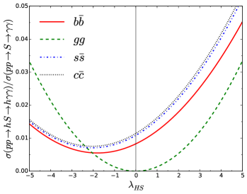
Figure 3: The ratios $\rho(gg)$, $\rho(b\mathrm{bar}{b})$, $\rho(s\mathrm{bar}{s})$ and $\rho(c\mathrm{bar}{c})$ for $gg$, $b\mathrm{bar}{b}$, $s\mathrm{bar}{s}$ and $c\mathrm{bar}{c}$ initial states respectively, defined between the associated production $pp\rightarrow hS\rightarrow h\gamma\gamma$ and the single production $pp\rightarrow S\rightarrow\gamma\gamma$, as functions of the portal coupling $\lambda_{HS}$. The mass of the scalar resonance was taken to be $M=750$ GeV and the width $\Gamma=1$ GeV.

We show the dependence of the ratio $\rho$ on the portal coupling $\lambda_{HS}$ in Fig. 3 for $gg$, $b\mathrm{bar}{b}$, $s\mathrm{bar}{s}$ and $c\mathrm{bar}{c}$ initial states for the example di-photon resonance mass $M=750$ GeV and width $\Gamma=1$ GeV. A width of $\Gamma\lesssim 1$ GeV can be obtained for example, if $c_{\gamma}^{S}\sim\mathcal{O}(10)$ and $c_{G}\sim\mathcal{O}(1)$ or $(y_{d}^{S})^{33}\sim\mathcal{O}(1)$, for $\Lambda=1$ TeV, with a cross section in $pp\rightarrow\gamma\gamma$ compatible with current constraints. Similar behaviour of the ratio $\rho$ is obtained for different scalar $S$ masses and widths.

Since the dominant matrix-element contribution to the $gg$-initiated $hS$ process is proportional to the portal coupling, the process approximately vanishes as $\lambda_{HS}\rightarrow 0$, and hence $\rho(gg)\simeq\rho_{2gg}\lambda_{HS}^{2}$, where $\rho_{2gg}\approx 0.00133$, for $M=750$ GeV and $\Gamma=1$ GeV, obtained by performing a quadratic fit of the $gg$ curve in Fig. 3. As already discussed, this does not hold for the $q\mathrm{bar}{q}$-initiated process due to the contact interaction diagram. This results in a non-negligible minimum for $\rho(q\mathrm{bar}{q})$. A fit to the cross section, again for $M=750$ GeV and $\Gamma=1$ GeV, yields $\rho(q\mathrm{bar}{q})\simeq\rho_{2q\mathrm{bar}{q}}\lambda_{HS}^{2}+\rho_{1q\mathrm{bar}{q}}\lambda_{HS}+\rho_{0q\mathrm{bar}{q}}$ with $\rho_{0b\mathrm{bar}{b}}\approx 0.00828$, $\rho_{1b\mathrm{bar}{b}}\approx 0.00309$, $\rho_{2b\mathrm{bar}{b}}\approx 0.00086$, corresponding to $b\mathrm{bar}{b}$ initial states, and $\rho_{0s\mathrm{bar}{s}}\approx 0.01025$, $\rho_{1s\mathrm{bar}{s}}\approx 0.00371$, $\rho_{2s\mathrm{bar}{s}}\approx 0.00091$, corresponding to $s\mathrm{bar}{s}$ initial states. The case of $c\mathrm{bar}{c}$ is similar to the $s\mathrm{bar}{s}$ case and therefore in the rest of the article we focus on the cases $q=b$ and $q=s$. The positivity of the coefficient $\rho_{1q\mathrm{bar}{q}}$ indicates constructive interference between the contact interaction and resonant diagrams (for $\lambda_{HS}>0$). For an extended fit of the ratio $\rho$, including additional diagrams with the production of an intermediate Higgs boson due to ${\cal S}|H|^{2,4}$ interactions, that turn out to be sub-dominant, see Appendix B.

The fact that for quark-anti-quark annihilation the $hS$ process is non-vanishing for all values of the portal coupling $\lambda_{HS}$ indicates that one could employ this final state to exclude $b\mathrm{bar}{b}$, $s\mathrm{bar}{s}$ or $c\mathrm{bar}{c}$ annihilation as the dominant production process. The analysis that will follow in the present article suggests however, that the di-photon decay of the $S$ alone may not be sufficient for that purpose for the benchmark points that we consider.

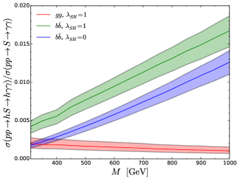
Figure 4: The ratios $\rho(gg)$ and $\rho(b\mathrm{bar}{b})$ for $gg$ and $b\mathrm{bar}{b}$ initial states, defined between the associated production $pp\rightarrow hS\rightarrow h\gamma\gamma$ and the single production $pp\rightarrow S\rightarrow\gamma\gamma$, as functions of the mass of the resonance, for $\Gamma=1$ GeV. The bands display the parton density function uncertainty for the MMHT14nlo68cl set combined in quadrature with the scale variation between 0.5 and 2.0 times the default central dynamical scale implemented in MadGraph5_aMC@NLO.

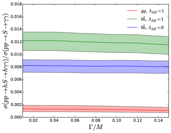
Figure 5: The ratios $\rho(gg)$ and $\rho(b\mathrm{bar}{b})$ for $gg$ and $b\mathrm{bar}{b}$ initial states, defined between the associated production $pp\rightarrow hS\rightarrow h\gamma\gamma$ and the single production $pp\rightarrow S\rightarrow\gamma\gamma$, as functions of the width of the resonance over the mass, $\Gamma/M$. The bands display the parton density function uncertainty for the MMHT14nlo68cl set combined in quadrature with the scale variation between 0.5 and 2.0 times the default central dynamical scale implemented in MadGraph5_aMC@NLO. The scalar resonance mass was chosen to be $M=750$ GeV.

We show in Fig. 4 the variation of the ratio $\rho$ with the mass of the resonance, $M$, for the $gg$-iniated process and $\lambda_{HS}=1$, and for the $b\mathrm{bar}{b}$-initiated process for $\lambda_{HS}=0$ (no portal) and $\lambda_{HS}=1$. We have fixed the width to $\Gamma=1$ GeV. Interestingly, the pure $q\mathrm{bar}{q}$-induced processes exhibit an increase of the ratio $\rho$ with increasing mass – related to the new $q\mathrm{bar}qhS$ interaction growing with momentum – whereas the pure $gg$-induced process exhibits a slight decrease.

If the di-photon resonance is wide, the analyses performed for the $hS$ final state will differ in the details due to changes in the kinematics. We show in Fig. 5 the variation of the ratio $\rho$ with the width over the mass, $\Gamma/M$, at a fixed mass $M=750$ GeV, for $\lambda_{HS}=1$, and for the $b\mathrm{bar}{b}$-initiated process for $\lambda_{HS}=0$ (no portal) and $\lambda_{HS}=1$. One can observe that the central value of the ratio remains approximately constant in all cases, with only a slight decrease with increasing width.

In both Figs. 4 and 5, we also provide, as coloured bands, the parton density function uncertainty for the MMHT14nlo68cl set Motylinski et al. (2014) combined in quadrature with the scale variation between 0.5 and 2.0 times the default central dynamical scale implemented in MadGraph5_aMC@NLO. For a mass of 750 GeV, the total theoretical uncertainties due to scale and PDF variations are $\sim^{+40}_{-30}\%$ for the $gg$-induced process, $\sim\pm 10\%$ for the $b\mathrm{bar}{b}$-induced and $\sim\pm 30\%$ for the $s\mathrm{bar}{s}$-induced cases (the latter not shown in the figure for simplicity).

Assuming a total cross section for the production of a $\gamma\gamma$ resonance of mass $M=750$ GeV of, say, $\sigma(pp\rightarrow S\rightarrow\gamma\gamma)=5$ fb (see below), one would expect a total of $\mathcal{O}(20)$ $hS\rightarrow h\gamma\gamma$ events at the high-luminosity LHC (HL-LHC, assuming 3000 fb^-1 of integrated luminosity) if the process is gluon-fusion initiated and $\mathcal{O}(200)$ events for $b\mathrm{bar}{b}$-initiated production, for a portal coupling $\lambda_{HS}=1$. Moreover, the minimum expected number of events for the $b\mathrm{bar}{b}$-initiated process is $\mathcal{O}(80)$, arising for $\lambda_{HS}\simeq-1.8$ and for the $s\mathrm{bar}{s}$-initiated process one expects a minimum of $\mathcal{O}(100)$ events for $\lambda_{HS}\simeq-2.0$. We note here that the positions of the minima for the $q\mathrm{bar}{q}$-initiated process will change after cuts due to the varying effect of the analysis on the different pieces contributing to the cross section.

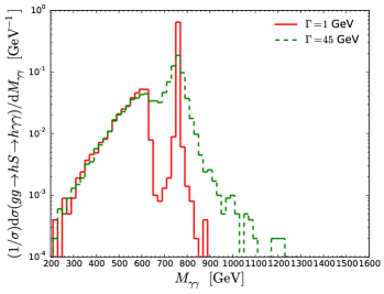
Figure 6: The matrix-element level distribution of the di-photon invariant mass, $M_{\gamma\gamma}$, in the $gg\rightarrow hS\rightarrow h\gamma\gamma$ process, normalised to unity, for the two different width scenarios, $\Gamma=1$ GeV and $\Gamma=45$ GeV, for $M=750$ GeV.

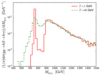
Figure 7: The matrix-element-level distribution of the combined Higgs boson and di-photon invariant mass, $M_{h\gamma\gamma}$, in the $gg\rightarrow hS\rightarrow h\gamma\gamma$ process, normalised to unity, for the two different width scenarios, $\Gamma=1$ GeV and $\Gamma=45$ GeV, for $M=750$ GeV.

The kinematic structure of the $pp\rightarrow hS\rightarrow h\gamma\gamma$ process can be well-described by examining the distribution of the invariant mass of the $\gamma\gamma$ state, $M_{\gamma\gamma}$, or the distribution of the invariant mass of the Higgs boson and di-photon combination, $M_{h\gamma\gamma}$. In Figs. 6 and 7 we show, respectively, these distributions for the gluon-fusion-initiated process, for two widths, $\Gamma=1$ GeV, $\Gamma=45$ GeV. For the sake of clarity, here we only show distributions for a scalar mass of $M=750$ GeV, but the main features remain unaltered as long as the scalar is heavier than the Higgs boson, $M>M_{h}$. The distributions clearly show the existence of two regions: a region in which the intermediate $s$-channel propagator for the $S$ scalar is on-shell and the final-state $S(\gamma\gamma)$ is off-shell, and a region in which the $s$-channel internal propagator is instead off-shell and the final-state $S(\gamma\gamma)$ is on-shell. The existence of the former region, $M_{\gamma\gamma}\lesssim M-M_{h}$, $M_{h\gamma\gamma}\sim M$ which henceforth we will call “three-body decay” since the intermediate $S$ is decaying approximately on-shell, is made possible by the fact that the mass of the particle produced in association with $S$, the Higgs boson, is smaller than the masses of $S$ we are considering, $M>M_{h}=125$ GeV. The other region, $M_{\gamma\gamma}\sim M$, $M_{h\gamma\gamma}\gtrsim M+M_{h}$ which we will refer to as “on-shell di-photon”, exists irrespective of the mass of $S$. Note that both the three-body decay and on-shell di-photon regions exist even for $\Gamma/M\ll 1$. The normalised distributions look identical for all values of the portal coupling, $\lambda_{HS}$ ($\neq 0$), since the dominant contribution stems by far from the diagram shown in Fig. 1 (a).

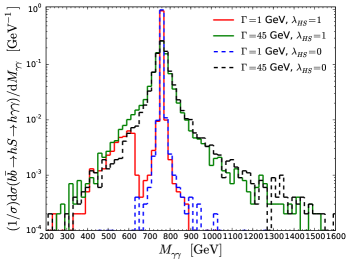
Figure 8: The matrix-element-level distribution of the di-photon invariant mass, $M_{\gamma\gamma}$, in the $b\mathrm{bar}{b}\rightarrow hS\rightarrow h\gamma\gamma$ process, normalised to unity, for two width scenarios, $\Gamma=1,~{}45$ GeV and two values of the portal coupling, $\lambda_{HS}=0,~{}1$, for $M=750$ GeV.

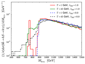
Figure 9: The matrix-element level distribution of the combined Higgs boson and di-photon invariant mass, $M_{h\gamma\gamma}$, in the $b\mathrm{bar}{b}\rightarrow hS\rightarrow h\gamma\gamma$ process, normalised to unity, for two width scenarios, $\Gamma=1,~{}45$ GeV and two values of the portal coupling, $\lambda_{HS}=0,~{}1$, for $M=750$ GeV.

In Figs. 8 and 9 we show the di-photon invariant mass and the combined Higgs boson and di-photon invariant mass for the $b\mathrm{bar}{b}$-initiated process, respectively, for $M=750$ GeV. Evidently the two regions observed for the $gg$ case are clearly still present for $\lambda_{HS}\neq 0$ and $\Gamma=1$ GeV, with the on-shell di-photon region dominating. For $\lambda_{HS}=0$, the “three-body decay” region disappears completely since the resonant $s$-channel diagram of Fig. 2 (a) vanishes. For large width the two regions merge into one and the effect of the vanishing three-body decay region for $\lambda_{HS}=0$ is not as evident as in the case of small width. The distributions for the $s\mathrm{bar}{s}$-initiated process exhibit similar features, with different “mixtures” between the two regions arising from the differences between the strange and bottom quark parton density functions. We omit them for the sake of simplicity.

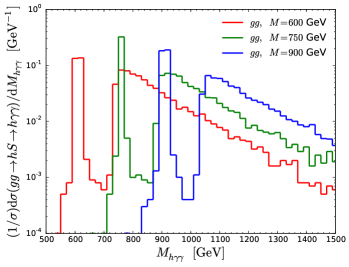
Figure 10: The matrix-element level distribution of the combined Higgs boson and di-photon invariant mass, $M_{h\gamma\gamma}$, in the $gg\rightarrow hS\rightarrow h\gamma\gamma$ process, normalised to unity, for three benchmark mass scenarios, $M=600,~{}750,~{}900$ GeV, and $\Gamma=1$ GeV.

Figure 11: The matrix-element level distribution of the combined Higgs boson and di-photon invariant mass, $M_{h\gamma\gamma}$, in the $b\mathrm{bar}{b}\rightarrow hS\rightarrow h\gamma\gamma$ process, normalised to unity, for three benchmark mass scenarios, $M=600,~{}750,~{}900$ GeV, and $\Gamma=1$ GeV, for $\lambda_{HS}=1$.

Figures 10 and 11 show the distributions of the combined invariant mass of the Higgs boson and di-photon, $M_{h\gamma\gamma}$, for the pure $gg$-initiated and pure $b\mathrm{bar}{b}$-initiated cases respectively, for the three values of the scalar mass that we will consider as “benchmark” scenarios in our analysis, $M=600,~{}750,~{}900$ GeV (see below) and $\Gamma=1$ GeV. For the $b\mathrm{bar}{b}$ case we only show the $\lambda_{HS}=1$ distributions for simplicity. They all clearly demonstrate the existence of the main features described for the $M=750$ GeV case, i.e. the “three-body decay” and “on-shell di-photon” regions.

III Event generation and detector simulation.

III.1 Event generation.

The signal model was generated via an implementation of the Lagrangian of Eq. I in FeynRules Christensen and Duhr (2009); Alloul et al. (2014). Via the UFO interface Degrande et al. (2012) this was used to generate parton-level events employing MadGraph5_aMC@NLO Alwall et al. (2011, 2014). The background processes were also generated using MadGraph5_aMC@NLO, with appropriate generation-level cuts to reduce the initial cross sections to a manageable level. All the events were passed through the HERWIG 7 Bahr et al. (2008); Gieseke et al. (2011); Arnold et al. (2012); Bellm et al. (2013, 2016) Monte Carlo for simulation of the parton shower, the underlying event and hadronization. As before, the MMHT14nlo68cl PDF set was employed. To remain conservative, we consider collisions at the LHC at a centre-of-mass energy of 13 TeV. The possible increase of energy to 14 TeV will increase rates in the considered processes by $\mathcal{O}(10\%)$.

Since we expect to impose cuts on the di-photon mass window, $M_{\gamma\gamma}$, that are sufficiently far away from the Higgs boson resonance, we can immediately exclude any background processes containing $h\rightarrow\gamma\gamma$ from the analysis. For this reason we do not include associated Higgs boson production with a vector boson or Higgs boson pair production, $t\mathrm{bar}{t}h$ production, and so on. This implies that the relevant backgrounds are those with non-resonant $\gamma\gamma$ production, other processes that involve $S\rightarrow\gamma\gamma$, and reducible backgrounds. We thus consider the following processes: $\gamma+$jets, $\gamma\gamma+$jets, events with at least one true $b$-quark at parton-level ($b$+jets), $Z\gamma\gamma$ with $Z\rightarrow b\mathrm{bar}{b}$, $t\mathrm{bar}{t}\gamma\gamma$ including all the decay modes of the top quarks and the production of the resonance $S$ in association with a non-resonant $b\mathrm{bar}{b}$ pair. All the multi-jet processes are generated without merging to the parton shower, in the five-flavour scheme, with four outgoing partons at the matrix-element level.

The calculation of higher-order QCD corrections to these multi-leg processes, particularly when restricting the phase space with cuts, is numerically challenging at present. To remain conservative, we will assume that the corrections are large and apply $K$-factors of $K=2$ to all the background processes. For the signal and the $b\mathrm{bar}{b}S$ associated production we do not apply any $K$-factors since the corrections are approximately absorbed into the ratio with the single inclusive production of the $S$ resonance, see below. Throughout this article we assume that $\sigma(pp\rightarrow S\rightarrow\gamma\gamma)=10,~{}5,~{}1$ fb, corresponding to the benchmark masses $M=600,~{}750,~{}900$ GeV, fixing the product $c_{G}^{S}c_{\gamma}^{S}$ (or $(y_{d}^{S})^{ii}c_{\gamma}^{S}$), which drops out in the ratio $\rho$. The values of the cross sections are motivated by the current ATLAS ATL (2016b) and CMS Khachatryan et al. (2016) limits on di-photon resonances.

Note that it turns out that the non-resonant $b\mathrm{bar}{b}S$ process is only relevant for gluon-fusion production of $S$, and we only report numbers for that in what follows.

III.2 Detector simulation.

In the hadron-level analysis that follows, performed without using any dedicated detector simulation software, we consider all particles within a pseudo-rapidity of $|\eta|<5$ and $p_{T}>100$ MeV. We smear the momenta of all reconstructed objects (i.e. jets, electrons, muons and photons) according to HL-LHC projections The (2013a, b). We also apply the relevant reconstruction efficiencies. We simulate $b$-jet tagging by looking for jets containing $B$-hadrons, that we have set to stable in the simulation, and considering them as the $b$-jet candidates. The mis-tagging of $c$-jets to $b$-jets is performed by choosing $c$-jet candidates (after hadronization) as those jets that lie within a distance $\Delta R<0.4$ from $c$-quarks (after the parton shower), with transverse momentum $p_{T}>1$ GeV. We apply a flat b-tagging efficiency of 70% and a mis-tag rate of 1% for light-flavour jets and 10% for charm-quark-initiated jets.

We reconstruct jets using the anti-$k_{t}$ algorithm available in the FastJet package Cacciari et al. (2012); Cacciari and Salam (2006), with a radius parameter of $R=0.4$. We only consider jets, photons and leptons with $p_{T}>30$ GeV within pseudo-rapidity $|\eta|<2.5$ in our analysis. The jet-to-lepton mis-identification probability is taken to be $\mathcal{P}_{j\rightarrow\ell}=0.0048\times\mathrm{e}^{-0.035p_{Tj}/\mathrm{GeV}}$ and the jet-to-photon mis-identification probability was taken to be $\mathcal{P}_{j\rightarrow\gamma}=0.0093\times\mathrm{e}^{-0.036p_{Tj}/\mathrm{GeV}}$ The (2013a, b), both flat in pseudo-rapidity. We demand all leptons and photons to be isolated, where an isolated object is defined to have $\sum_{i}p_{T,i}$ less than 15% of its transverse momentum in a cone of $\Delta R=0.2$ around it.

IV Detailed analysis.

We consider events with two reconstructed $b$-jets and two isolated photons as defined in Section III. Note that this final state has been previously considered in the context of searches for Higgs boson pair production, e.g. in Baur et al. (2004); Baglio et al. (2013); Yao (2013); Barger et al. (2014); Chen et al. (2014). We impose the following ‘acceptance’ cuts to all samples:

• $b$-jets: transverse momenta $p_{T,b1}>30$ GeV, $p_{T,b2}>30$ GeV, all $b$-jets within $|\eta|<2.5$,

• photons: transverse momenta $p_{T,\gamma 1}>30$ GeV, $p_{T,\gamma 2}>30$ GeV, all photons within $|\eta|<2.5$,

• invariant mass of the two $b$-jets $M_{b\mathrm{bar}{b}}\in[90,160]$ GeV,

• invariant mass of the two photons $M_{\gamma\gamma}>M-300$ GeV,

• veto events with leptons of $p_{T}>25$ GeV within $|\eta|<2.5$,

for each of the considered di-photon resonance masses, $M$.

process	acceptance $\sigma$ [fb]
$gg\rightarrow h(b\mathrm{bar}{b})S(\gamma\gamma)$, $\Gamma=1$ GeV, $\lambda_{HS}=1$	0.00054
$gg\rightarrow h(b\mathrm{bar}{b})S(\gamma\gamma)$, $\Gamma=45$ GeV, $\lambda_{HS}=1$	0.00055
$b\mathrm{bar}{b}\rightarrow h(b\mathrm{bar}{b})S(\gamma\gamma)$, $\Gamma=1$ GeV, $\lambda_{HS}=1$	0.00266
$b\mathrm{bar}{b}\rightarrow h(b\mathrm{bar}{b})S(\gamma\gamma)$, $\Gamma=45$ GeV, $\lambda_{HS}=1$	0.00254
$b\mathrm{bar}{b}\rightarrow h(b\mathrm{bar}{b})S(\gamma\gamma)$, $\Gamma=1$ GeV, $\lambda_{HS}=0$	0.00184
$b\mathrm{bar}{b}\rightarrow h(b\mathrm{bar}{b})S(\gamma\gamma)$, $\Gamma=45$ GeV, $\lambda_{HS}=0$	0.00172
$s\mathrm{bar}{s}\rightarrow h(b\mathrm{bar}{b})S(\gamma\gamma)$, $\Gamma=1$ GeV, $\lambda_{HS}=1$	0.00366
$s\mathrm{bar}{s}\rightarrow h(b\mathrm{bar}{b})S(\gamma\gamma)$, $\Gamma=45$ GeV, $\lambda_{HS}=1$	0.00370
$s\mathrm{bar}{s}\rightarrow h(b\mathrm{bar}{b})S(\gamma\gamma)$, $\Gamma=1$ GeV, $\lambda_{HS}=0$	0.00291
$s\mathrm{bar}{s}\rightarrow h(b\mathrm{bar}{b})S(\gamma\gamma)$, $\Gamma=45$ GeV, $\lambda_{HS}=0$	0.00249
at least one $b$-quark + jets	0.31300
$\gamma$ + jets	0.11259
$\gamma\gamma$ + jets	0.15766
$Z\gamma\gamma\rightarrow(b\mathrm{bar}{b})\gamma\gamma$	0.00489
$t\mathrm{bar}{t}\gamma\gamma$	0.00281
$gg\rightarrow b\mathrm{bar}{b}S(\gamma\gamma)$, $\Gamma=1$ GeV	0.00058
$gg\rightarrow b\mathrm{bar}{b}S(\gamma\gamma)$, $\Gamma=45$ GeV	0.00063

Table 1: The expected cross sections at 13 TeV $pp$ collision energy for all the considered processes after acceptance cuts for $M=750$ GeV and $\Gamma=1,~{}45$ GeV. All branching ratios, acceptances and tagging rates have been applied. We have assumed that the single production cross section for a di-photon scalar resonance of $M=750$ GeV is $\sigma(pp\rightarrow S\rightarrow\gamma\gamma)=5$ fb.

The cross sections after application of the acceptance cuts are given in Table 1 for two values of the widths $\Gamma=1$ GeV and $\Gamma=45$ GeV and for $M=750$ GeV. For the case of $q\mathrm{bar}{q}$ we consider as examples $\lambda_{HS}=1$ and $\lambda_{HS}=0$. Throughout this analysis, the total signal cross section was calculated by using the ratio $\rho$ (derived in Section II) as $\sigma(pp\rightarrow hS\rightarrow h\gamma\gamma)=\rho\times\sigma(pp\rightarrow S\rightarrow\gamma\gamma)$, where $\sigma(pp\rightarrow S\rightarrow\gamma\gamma)=10,~{}5,~{}1$ fb for $M=600,~{}750,~{}900$ GeV, and including the decay $h\to b\mathrm{bar}b$. This cross section was employed as the normalisation of the signal event samples (before analysis cuts). The expected number of signal events, for $\lambda_{HS}\sim\mathcal{O}(1)$, after acceptance cuts is $\mathcal{O}(1)-\mathcal{O}(10)$ at 3000 fb^-1 of integrated luminosity. However, as already discussed, one should keep in mind that the cross section grows with $\lambda_{HS}^{2}$ in both $gg$- and $q\mathrm{bar}{q}$-initiated production.

Figure 12: The distribution of the di-photon invariant mass, $M_{\gamma\gamma}$, for the $gg\rightarrow hS\rightarrow b\mathrm{bar}b\gamma\gamma$ process after acceptance cuts, normalised to unity, for two width scenarios, $\Gamma=1$ GeV and $\Gamma=45$ GeV, while $M=750$ GeV.

Figure 13: The distribution of the combined di-photon + $b\mathrm{bar}b$ invariant mass, $M_{b\mathrm{bar}b\gamma\gamma}$, for the $gg\rightarrow hS\rightarrow b\mathrm{bar}b\gamma\gamma$ process after acceptance cuts, normalised to unity, for two width scenarios, $\Gamma=1$ GeV and $\Gamma=45$ GeV, while $M=750$ GeV.

The resulting di-photon invariant mass after acceptance cuts is shown in Fig. 12 for the example of $M=750$ GeV. The $M_{\gamma\gamma}$ observable can be used to separate the analysis into the two regions described in Section II: the “three-body decay” region (“TBD”) and the “on-shell di-photon” region (“OS$\gamma\gamma$”). The separation is identical in both $gg$- and $q\mathrm{bar}{q}$-initiated processess. We choose: $M_{\gamma\gamma}<M-50$ GeV for the “TBD” region and $M_{\gamma\gamma}>M-50$ GeV for the “OS$\gamma\gamma$” region for a di-photon resonance mass, $M$. We also show the distribution of the combined invariant mass of the two $b$-jet candidates and the di-photon system, $M_{b\mathrm{bar}{b}\gamma\gamma}$ in Fig. 13, which also clearly demonstrates the existence of the two regions.

We apply further cuts to improve signal and background discrimination. As we did not attempt to fully optimize the cuts in the present analysis, we apply a common set of cuts along with invariant mass cuts on the observables $M_{\gamma\gamma}$ and $M_{b\mathrm{bar}{b}\gamma\gamma}$ that provide the main distinction between the two regions. The common cuts applied in each region are shown in Table 2 and the specific invariant mass cuts are shown in Table 3. Effectively, the cuts aim to exploit the fact that the photons in the signal are harder than in the backgrounds and also feature tighter di-photon and $b\mathrm{bar}{b}$ mass windows, particularly in the “OS$\gamma\gamma$” region for the former.

observable	cut
$p_{T,\gamma 1}$	$>200$ GeV
$p_{T,\gamma 2}$	$>120$ GeV
$\Delta R(\gamma,\gamma)$	$\in[2.0,4.0]$
$M_{b\mathrm{bar}{b}}$	$\in[100,150]$ GeV
$\Delta R(b,\mathrm{bar}{b})$	$\in[0.8,3.0]$
$\Delta R(\gamma\gamma,b_{2})$	$<3.0$

Table 2: The additional common cuts applied along with the acceptance cuts in both the “three-body decay” and the “on-shell di-photon” region for the $gg$- and $q\mathrm{bar}{q}$-initiated processess. The labels “$1$” and “$2$” correspond to the hardest and second hardest reconstructed objects (photons or $b$-jets), respectively.

	“TBD’	“OS$\gamma\gamma$”
$\Gamma=1$ GeV
$M_{\gamma\gamma}$	$\in M_{-300}^{-110}$ GeV	$\in M\pm 5$ GeV
$M_{b\mathrm{bar}{b}\gamma\gamma}$	$\in M\pm 30$ GeV	-
$\Gamma=45$ GeV:
$M_{\gamma\gamma}$	$\in M^{-110}_{-300}$ GeV	$\in M\pm 40$ GeV
$M_{b\mathrm{bar}{b}\gamma\gamma}$	$\in M\pm 40$ GeV	-

Table 3: The additional invariant mass cuts applied along with the further cuts of Table 2, in the “three-body decay” region (“TBD”) and the “on-shell di-photon” region (“OS$\gamma\gamma$”), for both the $gg$- and $q\mathrm{bar}{q}$-initiated processess for a scalar di-photon resonance of mass $M$. The different choices for the mass windows were made according to the width of the resonance, $\Gamma$.

process	“TBD”	“OS$\gamma\gamma$”
$gg\rightarrow h(b\mathrm{bar}{b})S(\gamma\gamma)$, $\Gamma=1$ GeV, $\lambda_{HS}=1$	0.00007	0.00020
$gg\rightarrow h(b\mathrm{bar}{b})S(\gamma\gamma)$, $\Gamma=45$ GeV, $\lambda_{HS}=1$	0.00006	0.00014
$b\mathrm{bar}{b}\rightarrow h(b\mathrm{bar}{b})S(\gamma\gamma)$, $\Gamma=1$ GeV, $\lambda_{HS}=1$	0.00007	0.00105
$b\mathrm{bar}{b}\rightarrow h(b\mathrm{bar}{b})S(\gamma\gamma)$, $\Gamma=45$ GeV, $\lambda_{HS}=1$	0.00038	0.00074
$b\mathrm{bar}{b}\rightarrow h(b\mathrm{bar}{b})S(\gamma\gamma)$, $\Gamma=1$ GeV, $\lambda_{HS}=0$	0	0.00064
$b\mathrm{bar}{b}\rightarrow h(b\mathrm{bar}{b})S(\gamma\gamma)$, $\Gamma=45$ GeV, $\lambda_{HS}=0$	0.00018	0.00055
$s\mathrm{bar}{s}\rightarrow h(b\mathrm{bar}{b})S(\gamma\gamma)$, $\Gamma=1$ GeV, $\lambda_{HS}=1$	0.00005	0.00134
$s\mathrm{bar}{s}\rightarrow h(b\mathrm{bar}{b})S(\gamma\gamma)$, $\Gamma=45$ GeV, $\lambda_{HS}=1$	0.00005	0.00107
$s\mathrm{bar}{s}\rightarrow h(b\mathrm{bar}{b})S(\gamma\gamma)$, $\Gamma=1$ GeV, $\lambda_{HS}=0$	0	0.00101
$s\mathrm{bar}{s}\rightarrow h(b\mathrm{bar}{b})S(\gamma\gamma)$, $\Gamma=45$ GeV, $\lambda_{HS}=0$	0.00003	0.00072
at least one $b$-quark + jets	$\mathcal{O}(10^{-7})$	$\mathcal{O}(10^{-10})$
$\gamma$ + jets	0.00025	$\mathcal{O}(10^{-7})$
$\gamma\gamma$ + jets	0.00182	0.00003
$Z\gamma\gamma\rightarrow(b\mathrm{bar}{b})\gamma\gamma$	$6\times 10^{-5}$	$10^{-5}$
$t\mathrm{bar}{t}\gamma\gamma$	$9\times 10^{-5}$	$10^{-5}$
$gg\rightarrow b\mathrm{bar}{b}S(\gamma\gamma)$, $\Gamma=1$ GeV	$\lesssim\mathcal{O}(10^{-6})$	0.00020
$gg\rightarrow b\mathrm{bar}{b}S(\gamma\gamma)$, $\Gamma=45$ GeV	$\mathcal{O}(10^{-6})$	0.00018

Table 4: The expected cross sections at 13 TeV $pp$ collision energy in fb for all the considered processes after the application of further cuts as in Tables 2 and 3, for $M=750$ GeV and $\Gamma=1,~{}45$ GeV. All branching ratios, acceptances and tagging rates have been applied. We have assumed that the single production cross section for a di-photon scalar resonance of $M=750$ GeV is $\sigma(pp\rightarrow S\rightarrow\gamma\gamma)=5$ fb.

We show the resulting cross sections after the application of these further cuts in Table 4, for the case of $M=750$ GeV. A high efficiency is maintained for the signal, with high rejection factors for the background processes. We note again that the $b\mathrm{bar}{b}S$ associated production process is relevant only for the gluon-fusion scenario.

To obtain the 95% confidence-level exclusion regions for $\lambda_{HS}$ we use Poissonian statistics to calculate the probabilities. Since we have assumed that the production of a scalar di-photon resonance will have been observed, we have to construct a null hypothesis compatible with such an observation providing the expected number of events at the LHC, that we will confront with the theory predictions in the parameter space to be tested. If these numbers differ by a certain significance, the corresponding point is expected to be excluded with this significance. In particular, any hypothesis has to be realistic and remain within the bounds of our model. Our underlying assumption is thus chosen to be that the scalar resonance $S$ is produced purely in gluon fusion to good approximation and that there is no portal coupling, $\lambda_{HS}=0$, which means there is basically no $h+S$ associated production. For further technical details on this statistical procedure, see Appendix C of Ref. Papaefstathiou et al. (2014). We do not incorporate the effect of systematic uncertainties on the signal or backgrounds. To perform a combination of the two analysis regions, “TBD” and “$OS\gamma\gamma$”, we employ the “Stouffer method” Stouffer et al. (1949), where the combined significance, $\Omega$, is given, in terms of the individual significances $\Omega_{i}$, as:

$$\Omega=\frac{1}{\sqrt{k}}\sum_{i=1}^{k}\Omega_{i}\;.$$ (8)

We show the resulting expected limits (assuming our null hypothesis is true) as a function of the integrated luminosity for the different benchmark scenarios that we consider in Figs. 14-25. For the case $M=750$ GeV we show results for $\Gamma=45$ GeV as well. For $\Gamma=1$ GeV, we obtain more stringent constraints, limiting, for $M=600,~{}750,~{}900$ GeV respectively, $|\lambda_{HS}|\lesssim 2,~{}4,~{}5$ for the $gg$-initiated process and $\lambda_{HS}\in[\sim-4,\sim 1],~{}[\sim-7,\sim 3],~{}[\sim-8,\sim 4]$, both for the $b\mathrm{bar}{b}$ and $s\mathrm{bar}{s}$-initiated processes, at the end of the HL-LHC run (3000 fb^-1). The variation between the results for $b\mathrm{bar}{b}$ and $s\mathrm{bar}{s}$-initiated processes – visible in the plots – is very small and can be attributed to the differences between the parton density functions for the strange and bottom quarks, as already mentioned.

The scenario with the larger width, $M=750$ GeV, $\Gamma=45$ GeV, clearly exhibits weaker constraints, with the $gg$-initiated processes yielding $|\lambda_{HS}|\lesssim 5$, the $b\mathrm{bar}{b}$-initiated process $\lambda_{HS}\in[\sim-8,\sim 5]$ and the $s\mathrm{bar}{s}$-initiated process $\lambda_{HS}\in[\sim-8,\sim 4]$. It is conceivable that if further decay channels of the resonance $S$ are discovered, the remaining unconstrained regions in the $q\mathrm{bar}q$ cases can be covered (in particular for narrow width), allowing determination of the initial state partons that produce the resonance.

The lower bound on $\lambda_{HS}$ for the $q\mathrm{bar}{q}$-initiated cases is driven by the “TBD” region. This is understood by the fact that the “TBD” region always vanishes near $\lambda_{HS}\sim 0$, as it is dominated by the diagram with an on-shell $s$-channel $S$, making the exclusion region resulting from it symmetric with respect to $\lambda_{HS}\sim 0$, whereas the “OS$\gamma\gamma$” region possesses a symmetry point somewhere in $\lambda_{HS}<0$.

Figure 14: The grey-shaded area shows the 95% confidence-level exclusion region for the portal coupling $\lambda_{HS}$ for the $gg$-induced case and $M=600$ GeV, $\Gamma=1$ GeV, for the combination of the “TBD” (red) and “OS$\gamma\gamma$” (green) regions as defined in the main text. We have assumed that the single production cross section $\sigma(pp\rightarrow S\rightarrow\gamma\gamma)=10$ fb.

Figure 15: The grey-shaded area shows the 95% confidence-level exclusion region for the portal coupling $\lambda_{HS}$ for the $b\mathrm{bar}{b}$-induced case and $M=600$ GeV, $\Gamma=1$ GeV, for the combination of the “TBD” (red) and “OS$\gamma\gamma$” (green) regions as defined in the main text. We have assumed that the single production cross section $\sigma(pp\rightarrow S\rightarrow\gamma\gamma)=10$ fb.

Figure 16: The grey-shaded area shows the 95% confidence-level exclusion region for the portal coupling $\lambda_{HS}$ for the $s\mathrm{bar}{s}$-induced case and $M=600$ GeV, $\Gamma=1$ GeV, for the combination of the “TBD” (red) and “OS$\gamma\gamma$” (green) regions as defined in the main text. We have assumed that the single production cross section $\sigma(pp\rightarrow S\rightarrow\gamma\gamma)=10$ fb.

Figure 17: The grey-shaded area shows the 95% confidence-level exclusion region for the portal coupling $\lambda_{HS}$ for the $gg$-induced case and $M=750$ GeV, $\Gamma=1$ GeV, for the combination of the “TBD” (red) and “OS$\gamma\gamma$” (green) regions as defined in the main text. We have assumed that the single production cross section $\sigma(pp\rightarrow S\rightarrow\gamma\gamma)=5$ fb.

Figure 18: The grey-shaded area shows the 95% confidence-level exclusion region for the portal coupling $\lambda_{HS}$ for the $gg$-induced case and $M=750$ GeV, $\Gamma=45$ GeV, for the combination of the “TBD” (red) and “OS$\gamma\gamma$” (green) regions as defined in the main text. We have assumed that the single production cross section $\sigma(pp\rightarrow S\rightarrow\gamma\gamma)=5$ fb.

Figure 19: The grey-shaded area shows the 95% confidence-level exclusion region for the portal coupling $\lambda_{HS}$ for the $b\mathrm{bar}{b}$-induced case and $M=750$ GeV, $\Gamma=1$ GeV, for the combination of the “TBD” (red) and “OS$\gamma\gamma$” (green) regions as defined in the main text. We have assumed that the single production cross section $\sigma(pp\rightarrow S\rightarrow\gamma\gamma)=5$ fb.

Figure 20: The grey-shaded area shows the 95% confidence-level exclusion region for the portal coupling $\lambda_{HS}$ for the $b\mathrm{bar}{b}$-induced case and $M=750$ GeV, $\Gamma=45$ GeV, for the combination of the “TBD” (red) and “OS$\gamma\gamma$” (green) regions as defined in the main text. We have assumed that the single production cross section $\sigma(pp\rightarrow S\rightarrow\gamma\gamma)=5$ fb.

Figure 21: The grey-shaded area shows the 95% confidence-level exclusion region for the portal coupling $\lambda_{HS}$ for the $s\mathrm{bar}{s}$-induced case and $M=750$ GeV, $\Gamma=1$ GeV, for the combination of the “TBD” (red) and “OS$\gamma\gamma$” (green) regions as defined in the main text. We have assumed that the single production cross section $\sigma(pp\rightarrow S\rightarrow\gamma\gamma)=5$ fb.

Figure 22: The grey-shaded area shows the 95% confidence-level exclusion region for the portal coupling $\lambda_{HS}$ for the $s\mathrm{bar}{s}$-induced case and $M=750$ GeV, $\Gamma=45$ GeV, for the combination of the “TBD” (red) and “OS$\gamma\gamma$” (green) regions as defined in the main text. We have assumed that the single production cross section $\sigma(pp\rightarrow S\rightarrow\gamma\gamma)=5$ fb.

Figure 23: The grey-shaded area shows the 95% confidence-level exclusion region for the portal coupling $\lambda_{HS}$ for the $gg$-induced case and $M=900$ GeV, $\Gamma=1$ GeV, for the combination of the “TBD” (red) and “OS$\gamma\gamma$” (green) regions as defined in the main text. We have assumed that the single production cross section $\sigma(pp\rightarrow S\rightarrow\gamma\gamma)=1$ fb.

Figure 24: The grey-shaded area shows the 95% confidence-level exclusion region for the portal coupling $\lambda_{HS}$ for the $b\mathrm{bar}{b}$-induced case and $M=900$ GeV, $\Gamma=1$ GeV, for the combination of the “TBD” (red) and “OS$\gamma\gamma$” (green) regions as defined in the main text. We have assumed that the single production cross section $\sigma(pp\rightarrow S\rightarrow\gamma\gamma)=1$ fb.

Figure 25: The grey-shaded area shows the 95% confidence-level exclusion region for the portal coupling $\lambda_{HS}$ for the $s\mathrm{bar}{s}$-induced case and $M=900$ GeV, $\Gamma=1$ GeV, for the combination of the “TBD” (red) and “OS$\gamma\gamma$” (green) regions as defined in the main text. We have assumed that the single production cross section $\sigma(pp\rightarrow S\rightarrow\gamma\gamma)=1$ fb.

Mixed production of the di-photon resonance

So far we have investigated production of the scalar resonance initiated purely either via gluon fusion or $q\mathrm{bar}{q}$ annihilation. We can generalize this to “mixed” production via $gg$ and $q\mathrm{bar}{q}$ initial states simultaneously. We concentrate on the scenario of $gg$ and $b\mathrm{bar}{b}$ for simplicity, with the extension to additional quark flavours being straightforward. In that case, the ratio of cross sections, $\rho_{\mathrm{mixed}}$, defined between the associated production and single production modes can be written as:

$$\rho_{\mathrm{mixed}} = \frac{\sigma(b\mathrm{bar}{b}\rightarrow hS\rightarrow h\gamma\gamma)+\sigma(gg\rightarrow hS\rightarrow h\gamma\gamma)}{\sigma(b\mathrm{bar}{b}\rightarrow S\rightarrow\gamma\gamma)+\sigma(gg\rightarrow S\rightarrow\gamma\gamma)}$$ (9)

$$= \frac{B_{2}(\lambda_{HS})[(y^{S}_{d})^{33}]^{2}+G_{2}(\lambda_{HS})(c_{G}^{S})^{2}}{B_{1}[(y^{S}_{d})^{33}]^{2}+G_{1}(c_{G}^{S})^{2}}\;,$$

where $B_{2}(\lambda_{HS})$, $G_{2}(\lambda_{HS})$ are functions of the portal coupling $\lambda_{HS}$ and $B_{1}$, $G_{1}$ are constants with respect to the portal coupling, all to be determined. Defining $\theta\equiv|[(y^{S}_{d})^{33}]/c_{G}^{S}|$, the above expression can be re-written as:

$$\rho_{\mathrm{mixed}}=\frac{B_{2}(\lambda_{HS})\theta^{2}+G_{2}(\lambda_{HS})}{B_{1}\theta^{2}+G_{1}}\;.$$ (10)

By considering the limits $\theta\rightarrow 0$ and $\theta\rightarrow\infty$, and dividing the numerator and denominator by $G_{1}$, we can deduce that

$$\rho_{\mathrm{mixed}}=\frac{\rho(b\mathrm{bar}{b},\lambda_{HS})r_{bg}\theta^{2}+\rho(gg,\lambda_{HS})}{r_{bg}\theta^{2}+1}\;,$$ (11)

where $\rho(b\mathrm{bar}{b},\lambda_{HS})$ and $\rho(gg,\lambda_{HS})$ are the ratios of cross sections as functions of the portal coupling as defined in Eq. 7, for the cases of pure production initiated either via $b\mathrm{bar}{b}$ or $gg$, respectively, and $r_{bg}$ is the ratio of pure single production cross sections for $\theta=1$: $r_{bg}=B_{1}/G_{1}$. The former two functions have already been determined in the analysis of the pure cases. The constant $r_{bg}$ was calculated explicitly via Monte Carlo to be $r_{bg}\approx 1.02,~{}0.69,~{}0.49$ for $M=600,~{}750,~{}900$ GeV respectively. The values are approximately equal for both the narrow width case ($\Gamma=1$ GeV) and the larger width case ($\Gamma=45$ GeV).

Figure 26: The 95% confidence-level exclusion region for the ratio of couplings to $b\mathrm{bar}{b}$ over the coupling to the $gg$ initial states, $\theta=[(y^{S}_{d})^{33}]/c_{G}^{S}$, versus the portal coupling $\lambda_{HS}$ for $M=600$ GeV, $\Gamma=1$ GeV. The excluded region coming from the combination of the “TBD” (red) and “OS$\gamma\gamma$” (green) regions is grey-shaded. We have assumed that the single production cross section $\sigma(pp\rightarrow S\rightarrow\gamma\gamma)=10$ fb.

Figure 27: The 95% confidence-level exclusion region for the ratio of couplings to $b\mathrm{bar}{b}$ over the coupling to the $gg$ initial states, $\theta=[(y^{S}_{d})^{33}]/c_{G}^{S}$, versus the portal coupling $\lambda_{HS}$ for $M=750$ GeV, $\Gamma=1$ GeV. The excluded region coming from the combination of the “TBD” (red) and “OS$\gamma\gamma$” (green) regions is grey-shaded. We have assumed that the single production cross section $\sigma(pp\rightarrow S\rightarrow\gamma\gamma)=5$ fb.

Figure 28: The 95% confidence-level exclusion region for the ratio of couplings to $b\mathrm{bar}{b}$ over the coupling to the $gg$ initial states, $\theta=[(y^{S}_{d})^{33}]/c_{G}^{S}$, versus the portal coupling $\lambda_{HS}$ for $M=900$ GeV, $\Gamma=1$ GeV. The excluded region coming from the combination of the “TBD” (red) and “OS$\gamma\gamma$” (green) regions is grey-shaded. We have assumed that the single production cross section $\sigma(pp\rightarrow S\rightarrow\gamma\gamma)=1$ fb.

Figure 29: The 95% confidence-level exclusion region for the ratio of couplings to $b\mathrm{bar}{b}$ over the coupling to the $gg$ initial states, $\theta=[(y^{S}_{d})^{33}]/c_{G}^{S}$, versus the portal coupling $\lambda_{HS}$ for $M=750$ GeV, $\Gamma=45$ GeV. The excluded region coming from the combination of the “TBD” (red) and “OS$\gamma\gamma$” (green) regions is grey-shaded. We have assumed that the single production cross section $\sigma(pp\rightarrow S\rightarrow\gamma\gamma)=5$ fb.

Using Eq. 11, we can deduce an expression for the predicted number of signal events after the application of analysis cuts in the mixed production case:

$$N_{\mathrm{mixed}}=\frac{r_{bg}\theta^{2}}{r_{bg}\theta^{2}+1}N(b\mathrm{bar}{b},\lambda_{HS})+\frac{1}{r_{bg}\theta^{2}+1}N(gg,\lambda_{HS})\;,$$ (12)

where $N(b\mathrm{bar}{b},\lambda_{HS})$ and $N(gg,\lambda_{HS})$ are the expected signal events for either pure $b\mathrm{bar}{b}$ or pure $gg$ production for a given value of $\lambda_{HS}$, at a specific integrated luminosity.

The predicted number of background events after a given set of analysis cuts is constant with $\theta$, apart from the associated production of the di-photon resonance with a $b\mathrm{bar}{b}$ pair, which was found to be significant only in the $gg$-initiated scenario. This background scales as $N_{\mathrm{assoc.}}=N_{assoc.,0}/(r_{bg}\theta^{2}+1)$, where $N_{assoc.,0}$ is the expected number of events for the $b\mathrm{bar}{b}S$ associated production after analysis cuts in the case of pure $gg$-initiated production.

Using the expression of Eq. 12 and the event numbers for the two analysis regions “TBD” and “OS$\gamma\gamma$” obtained for the pure production modes, we can derive constraints on the $(\theta,\lambda_{HS})$-plane. These are shown in Figs. 26-28 and 29, for masses $M=600,~{}750,~{}900$ GeV and $\Gamma=1$ GeV and for $M=750$ GeV and $\Gamma=45$ GeV, respectively, at an integrated luminosity of 3000 fb^-1 at 13 TeV. It can be seen that in the limits $\theta\rightarrow 0$ and $\theta\gg 1$, corresponding to $gg$- or $b\mathrm{bar}{b}$-dominated production respectively, one can recover the pure production constraints of Figs. 14-25 obtained at 3000 fb^-1.

V Discussion and Conclusions.

We have investigated the associated production of a di-photon scalar resonance with a Higgs boson and have employed the $pp\rightarrow hS\rightarrow(b\mathrm{bar}{b})(\gamma\gamma)$ final state to obtain constraints on the portal coupling with the SM Higgs boson $\lambda_{HS}$, at the LHC. We have considered three benchmark scalar masses, $M=600,~{}750,~{}900$ GeV, and we have assumed that the inclusive single production cross section is $\sigma(pp\rightarrow S\rightarrow\gamma\gamma)=10,5,1$ fb, respectively, compatible with current experimental constraints. To construct expected constraints we considered the null hypothesis (i.e. the supposed ‘true’ underlying theory) to correspond to gluon-fusion-initiated production with vanishing portal coupling, $\lambda_{HS}=0$. We then first analysed the case of either pure gluon-fusion-induced production or production via quark-anti-quark annihilation. For gluon-fusion production one can impose constraints on the portal coupling at the end of the HL-LHC run of $|\lambda_{HS}|\lesssim 2,4,5$ for $M=600,~{}750,~{}900$ GeV, respectively, and $\Gamma=1$ GeV, while $|\lambda_{HS}|\lesssim 5$ in the case of large width ($\Gamma=45$ GeV) and $M=750$ GeV. For quark-anti-quark annihilation, the production of an on-shell scalar and the Higgs boson is enhanced by a contact interaction $\sim q\mathrm{bar}{q}hS$, originating from the same $D=5$ operator that mediates single ${\cal S}$ production. This implies that the cross section is non-negligible even for vanishing portal coupling $\lambda_{HS}=0$. This fact can be exploited to exclude the whole plane of $\lambda_{HS}$, thus excluding the hypothesised production via $q\mathrm{bar}{q}$ annihilation. For the case of $b\mathrm{bar}{b}$ we find that a region inside $\lambda_{HS}\in[\sim-4,\sim 1],~{}[\sim-7,\sim 3],~{}[\sim-8,\sim 4]$ for $M=600,~{}750,~{}900$ GeV, respectively, could remain unconstrained at the end of the HL-LHC in the narrow width scenario, while $\lambda_{HS}\in[\sim-8,\sim 5]$ for large width and $M=750$ GeV. For the case of $s\mathrm{bar}{s}$ annihilation we find the same unconstrained regions to good approximation for narrow width, while we obtain $\lambda_{HS}\in[\sim-8,\sim 4]$ in the case of large width, where $M=750$ GeV. We have also considered ‘mixed’ production via gluon fusion and $b\mathrm{bar}{b}$ annihilation and derived constraints on the plane of ratio of the corresponding couplings versus $\lambda_{HS}$ for an integrated luminosity of 3000 fb^-1.

Note that since a measurement of $\lambda_{HS}$ can straightforwardly be translated into a measurement of $\mu_{S}$, these numbers suggest that it is possible to exclude, for example, the scenario where the mass of $S$ stems from EWSB ($\mu_{S}=0$), which corresponds to $\lambda_{HS}=M^{2}/v^{2}\approx 5.9,9.3,13.4$ (still assuming linear terms in ${\cal S}$ to vanish). Furthermore, if additional decay modes of the resonance $S$ are discovered beyond $\gamma\gamma$, it is conceivable that a combined analysis in various channels would be able to exclude all possible values of $\lambda_{HS}$ - for the case of $q\mathrm{bar}q$ production - thus providing an independent method of determining the production mode. Conversely, the analysis of the present article demonstrates that if the production mechanism is constrained via alternative means, it will be possible to obtain meaningful constraints on the interaction of a new scalar resonance and the Higgs boson, allowing determination of its relation to electroweak symmetry breaking.

Appendix A The full set of operators.

In this appendix, we provide the full set of operators for the SM in the presence of an additional dynamical scalar singlet ${\cal S}$, up to $D=5$. The fact that ${\cal S}$ does not transform under the SM gauge group makes the construction straightforward: in the case that it is CP even (with CP-conserving interactions), each additional operator will consist of a gauge invariant SM operator, multiplied by powers of ${\cal S}$ (and potentially derivatives). This means that in particular that, schematically, ${\cal L}\supset{\cal L}_{\rm SM}+{\cal L}_{\rm SM}\cdot{\cal S}$. If all operators in the SM would be marginal, i.e., feature $D=4$, this would already correspond to the full Lagrangian at $D\leq 5$, connecting the SM with the new resonance. In turn, the only operators that are missing (up to pure NP terms) are those containing the single relevant (i.e., $D<4$) operator of the SM, $|H|^{2}$. This can be multiplied by up to three powers of ${\cal S}$ as well as by $\partial^{2}{\cal S}$ (the latter being equivalent via integration by parts to ${\cal S}\partial^{2}|H|^{2}$). This finally leads to the Lagrangian

$$\mathcal{L}_{\rm eff} = {\cal L}_{\rm SM}+\frac{1}{2}\partial_{\mu}{\cal S}\partial^{\mu}{\cal S}-\frac{1}{2}\mu_{S}^{2}{\cal S}^{2}$$ (13)

$$- \frac{\lambda^{\prime}_{S}}{2\sqrt{2}}v{\cal{S}}^{3}-\frac{\lambda_{S}}{4}{\cal{S}}^{4}-\lambda^{\prime}_{HS}v|H|^{2}{\cal{S}}-\lambda_{HS}|H|^{2}{\cal{S}}^{2}$$

$$- \frac{\cal{S}}{\Lambda}\left[c_{\lambda S}{\cal{S}}^{4}+c_{HS}|H|^{2}{\cal{S}}^{2}+c_{\lambda H}|H|^{4}\right]$$

$$- (y_{d}^{S})^{ij}\frac{\cal{S}}{\Lambda}\mathrm{bar}{Q}_{L}^{i}Hd_{R}^{j}-(y_{u}^{S})^{ij}\frac{\cal{S}}{\Lambda}\mathrm{bar}{Q}_{L}^{i}\tilde{H}u_{R}^{j}+\mathrm{h.c.}$$

$$- \frac{\cal{S}}{\Lambda}\frac{1}{16\pi^{2}}\left[g^{\prime 2}c_{B}^{S}B_{\mu\nu}B^{\mu\nu}+g^{2}c_{W}^{S}W^{I\mu\nu}W_{\mu\nu}^{I}\right.$$

$$+ \left.g_{S}^{2}c_{G}^{S}G^{a\mu\nu}G_{\mu\nu}^{a}\right]\,.$$

Note that we have used equations of motion/field redefinitions to eliminate the operators $\mathcal{S}/\Lambda(\partial^{\mu}{\cal S})^{2},\,\mathcal{S}/\Lambda|D_{\mu}H|^{2},\,\mathcal{S}/\Lambda\partial^{2}|H|^{2}$ and those of type ${\cal S}/\Lambda\,\mathrm{bar}{q}D_{\mu}\gamma^{\mu}q$. The couplings in the third line of (13) and $\lambda^{\prime}_{S,HS}$, which are those that have been neglected in (I), do not contribute to the process under consideration to good approximation: They either do not enter at leading order, or (in the case of the $|H|^{2,4}{\cal S}$ interactions) at most contribute to a diagram with a (strongly suppressed) off-shell Higgs boson propagator, discussed in Appendix B. The same holds true for the $S^{4}$ term, that was kept for the discussion in Section I.

Appendix B Fits for the ratio $\rho$ including a linear term.

In addition to the diagrams of Figs. 1 and 2, there can be contributions to the final state under consideration originating from $hhS$ interactions (for example, an intermediate $s$-channel Higgs boson to $hS$ or an $S\to hh$ intermediate state), provided the following triple scalar interaction, linear in $S$, is non-vanishing:

$$-\kappa_{HS}vh^{2}S\subset-\lambda^{\prime}_{HS}v|H|^{2}{\cal{S}}-c_{\lambda H}\frac{\cal{S}}{\Lambda}|H|^{4}\;,$$ (14)

with $\kappa_{HS}=1/2\,\lambda^{\prime}_{HS}+3/(2\Lambda)\,c_{\lambda H}$.

In this scenario, terms will appear in the cross section ratio proportional to $\kappa_{HS}$ and $\kappa_{HS}^{2}$. Due to interference with the new $hhS$ diagrams (note that also the ‘non-signal’ $S\to hh$ interferes with the signal diagrams after an off-shell $h\to\gamma\gamma$), some dependence on the coupling of the resonance $S$ to photons, $c_{\gamma}^{S}$, as well as the production couplings, $(y_{d}^{S})^{22}$, $(y_{d}^{S})^{33}$ and $c_{G}^{S}$, is introduced in the denominator of the cross section ratio. Due to this, smaller values of $|c_{\gamma}^{S}|$ and the production couplings enhance the effect of the new contributions proportional to $\kappa_{HS}$ and $\kappa_{HS}^{2}$. To take these effects into account and at the same time remain conservative, we set $|c_{\gamma}^{S}|$ to the possible minimal value that produces a $\sigma(pp\to S\to\gamma\gamma)\sim 5\,{\text{fb}}$ for $M=750$ GeV, as derived in Ref. Gupta et al. (2015). This leads to $|c_{\gamma}^{S}|\gtrsim\{60,\,100,\,\,10\}$ for $s\mathrm{bar}{s}$, $b\mathrm{bar}{b}$ and $gg$ production, respectively, where here and in the following we assume a normalisation of $\Lambda=1\,$TeV. Moreover, one can derive conservative lower bounds on $|(y_{d}^{S})^{22}|$, $|(y_{d}^{S})^{33}|$ and $|c_{g}^{S}|$, by demanding $\sigma(pp\to S)\gtrsim 5\,$fb, leading to $|(y_{d}^{S})^{22}|\gtrsim 0.15$, $|(y_{d}^{S})^{33}|\gtrsim 0.2$ and $|c_{g}^{S}|\gtrsim 0.25$. We set these to their minimal values as well in what follows.

We can then parametrize the ratio $\rho(xx^{\prime})=\sigma(xx^{\prime}\rightarrow h\gamma\gamma)/\sigma(xx^{\prime}\rightarrow S\rightarrow\gamma\gamma),\,xx^{\prime}=b\mathrm{bar}b,s\mathrm{bar}s,gg$, by

$$\rho(xx^{\prime}) = \delta_{1}^{x}+\delta_{2}^{x}\,\kappa_{HS}\lambda_{HS}+\delta_{3}^{x}\,\kappa_{HS}$$ (15)

$$+ \delta_{4}^{x}\,\lambda_{HS}+\delta_{5}^{x}\,\kappa_{HS}^{2}+\delta_{6}^{x}\,\lambda_{HS}^{2}\;,$$

where $\delta_{i}^{b,s,g}$ are coefficients to be determined.

$i$	$\delta_{i}^{b}$	$\delta_{i}^{s}$	$\delta_{i}^{g}$
1	$8.27\times 10^{-3}$	$1.05\times 10^{-2}$	$<\mathcal{O}(10^{-5})$
2	$1.93\times 10^{-4}$	$-2.30\times 10^{-4}$	$\mathcal{O}(10^{-7})$
3	$8.26\times 10^{-4}$	$2.54\times 10^{-5}$	$<\mathcal{O}(10^{-6})$
4	$3.08\times 10^{-3}$	$3.71\times 10^{-3}$	$<\mathcal{O}(10^{-6})$
5	$2.40\times 10^{-5}$	$6.00\times 10^{-5}$	$<\mathcal{O}(10^{-8})$
6	$8.60\times 10^{-4}$	$9.27\times 10^{-4}$	$1.33\times 10^{-3}$

Table 5: The $\rho$ fit coefficients for the general case of including an interaction term proportional to $\mathcal{L}\supset-\kappa_{HS}vh^{2}S$ for width $\Gamma=1$ GeV and $M=750$ GeV.

An estimate of the coefficients in this conservative scenario, obtained numerically, is given in Table 5 for width $\Gamma=1$ GeV and $M=750$ GeV. The contributions from diagrams with an off-shell Higgs boson are a priori not fully negligible for the $b\mathrm{bar}{b}$-induced case, simply because of interference of the $s$-channel $h\to hS$ with the large matrix elements with the on-shell $S$ in the final state.

To investigate the size of $\kappa_{HS}$ that renders the off-shell Higgs boson contributions significant to the $pp\rightarrow h\gamma\gamma$ process, we consider the ratio $\rho(\kappa_{HS},\lambda_{HS})/\rho(\kappa_{HS}=0,\lambda_{HS})=1+r$, where $r$ is a number that characterises the fractional change in the ratio $\rho$ due to $\kappa_{HS}$ for a given value of $\lambda_{HS}$. If we choose $r=1$, which implies $\mathcal{O}(1)$ changes due to $\kappa_{HS}$, and solve for $\kappa_{HS}$ for values $\lambda_{HS}\sim\mathcal{O}(1)$ we obtain: $|\kappa_{HS}|\sim\{\mathcal{O}(10),\,\mathcal{O}(10),\,\mathcal{O}(10^{2})\}$ for $s\mathrm{bar}{s}$, $b\mathrm{bar}{b}$ and $gg$ production, respectively.

Since the gauge-invariant terms in the Lagrangian generating this coupling also induce a Higgs-scalar mixing, they can not be arbitrarily large. Indeed, Higgs data can constrain $|\kappa_{HS}|\lesssim 4$ at 95% confidence-level Carmi et al. (2012); Cheung et al. (2015); Bauer et al. (2016b). Therefore, given the values calculated in the previous paragraph, for $\kappa_{HS}$ to eventually have a non-negligible effect on the analysis of the present article, this bound needs to be violated, and setting $\kappa_{HS}=0$ is a justified approximation. Despite the fact that we focussed on $M=750$ GeV, the analysis is expected to give similar estimates for the other benchmark points considered in the main analysis of this article, $M=600,~{}900$ GeV.

References

- Falkowski et al. (2015) A. Falkowski, C. Gross, and O. Lebedev, JHEP 05, 057 (2015), arXiv:1502.01361 [hep-ph] .
- Bellazzini et al. (2014) B. Bellazzini, C. Csáki, and J. Serra, Eur. Phys. J. C74, 2766 (2014), arXiv:1401.2457 [hep-ph] .
- Bellazzini et al. (2016) B. Bellazzini, R. Franceschini, F. Sala, and J. Serra, JHEP 04, 072 (2016), arXiv:1512.05330 [hep-ph] .
- Ellwanger et al. (2010) U. Ellwanger, C. Hugonie, and A. M. Teixeira, Phys. Rept. 496, 1 (2010), arXiv:0910.1785 [hep-ph] .
- Hempfling (1996) R. Hempfling, Phys. Lett. B379, 153 (1996), arXiv:hep-ph/9604278 [hep-ph] .
- Englert et al. (2013) C. Englert, J. Jaeckel, V. V. Khoze, and M. Spannowsky, JHEP 04, 060 (2013), arXiv:1301.4224 [hep-ph] .
- Gherghetta et al. (2016) T. Gherghetta, N. Nagata, and M. Shifman, Phys. Rev. D93, 115010 (2016), arXiv:1604.01127 [hep-ph] .
- Tsumura and Velasco-Sevilla (2010) K. Tsumura and L. Velasco-Sevilla, Phys. Rev. D81, 036012 (2010), arXiv:0911.2149 [hep-ph] .
- Bauer et al. (2016a) M. Bauer, T. Schell, and T. Plehn, Phys. Rev. D94, 056003 (2016a), arXiv:1603.06950 [hep-ph] .
- Khachatryan et al. (2014) V. Khachatryan et al. (CMS), Eur. Phys. J. C74, 3076 (2014), arXiv:1407.0558 [hep-ex] .
- Aad et al. (2014) G. Aad et al. (ATLAS), Phys. Rev. D90, 112015 (2014), arXiv:1408.7084 [hep-ex] .
- ATL (2015) Search for resonances decaying to photon pairs in 3.2 fb-1 of collisions at = 13 TeV with the ATLAS detector, Tech. Rep. ATLAS-CONF-2015-081 (CERN, 2015).
- ATL (2016a) Search for resonances in diphoton events with the ATLAS detector at = 13 TeV, Tech. Rep. ATLAS-CONF-2016-018 (CERN, 2016).
- CMS (2015) Search for new physics in high mass diphoton events in proton-proton collisions at 13TeV, Tech. Rep. CMS-PAS-EXO-15-004 (CERN, 2015).
- CMS (2016) Search for new physics in high mass diphoton events in of proton-proton collisions at and combined interpretation of searches at and , Tech. Rep. CMS-PAS-EXO-16-018 (CERN, 2016).
- ATL (2016b) Search for scalar diphoton resonances with 15.4 fb-1 of data collected at =13 TeV in 2015 and 2016 with the ATLAS detector, Tech. Rep. ATLAS-CONF-2016-059 (CERN, 2016).
- Khachatryan et al. (2016) V. Khachatryan et al. (CMS), (2016), arXiv:1609.02507 [hep-ex] .
- Franceschini et al. (2016a) R. Franceschini, G. F. Giudice, J. F. Kamenik, M. McCullough, A. Pomarol, R. Rattazzi, M. Redi, F. Riva, A. Strumia, and R. Torre, JHEP 03, 144 (2016a), arXiv:1512.04933 [hep-ph] .
- Angelescu et al. (2016) A. Angelescu, A. Djouadi, and G. Moreau, Phys. Lett. B756, 126 (2016), arXiv:1512.04921 [hep-ph] .
- Knapen et al. (2016) S. Knapen, T. Melia, M. Papucci, and K. Zurek, Phys. Rev. D93, 075020 (2016), arXiv:1512.04928 [hep-ph] .
- Di Chiara et al. (2015) S. Di Chiara, L. Marzola, and M. Raidal, (2015), arXiv:1512.04939 [hep-ph] .
- McDermott et al. (2016) S. D. McDermott, P. Meade, and H. Ramani, Phys. Lett. B755, 353 (2016), arXiv:1512.05326 [hep-ph] .
- Ellis et al. (2016) J. Ellis, S. A. R. Ellis, J. Quevillon, V. Sanz, and T. You, JHEP 03, 176 (2016), arXiv:1512.05327 [hep-ph] .
- Gupta et al. (2015) R. S. Gupta, S. Jäger, Y. Kats, G. Perez, and E. Stamou, (2015), arXiv:1512.05332 [hep-ph] .
- Falkowski et al. (2016) A. Falkowski, O. Slone, and T. Volansky, JHEP 02, 152 (2016), arXiv:1512.05777 [hep-ph] .
- Alves et al. (2016) A. Alves, A. G. Dias, and K. Sinha, Phys. Lett. B757, 39 (2016), arXiv:1512.06091 [hep-ph] .
- Goertz et al. (2015) F. Goertz, J. F. Kamenik, A. Katz, and M. Nardecchia, (2015), arXiv:1512.08500 [hep-ph] .
- Son and Urbano (2015) M. Son and A. Urbano, (2015), arXiv:1512.08307 [hep-ph] .
- Gao et al. (2015) J. Gao, H. Zhang, and H. X. Zhu, (2015), arXiv:1512.08478 [hep-ph] .
- Salvio and Mazumdar (2016) A. Salvio and A. Mazumdar, Phys. Lett. B755, 469 (2016), arXiv:1512.08184 [hep-ph] .
- Gu and Liu (2016) J. Gu and Z. Liu, Phys. Rev. D93, 075006 (2016), arXiv:1512.07624 [hep-ph] .
- Djouadi et al. (2016) A. Djouadi, J. Ellis, R. Godbole, and J. Quevillon, JHEP 03, 205 (2016), arXiv:1601.03696 [hep-ph] .
- Salvio et al. (2016) A. Salvio, F. Staub, A. Strumia, and A. Urbano, JHEP 03, 214 (2016), arXiv:1602.01460 [hep-ph] .
- Gross et al. (2016) C. Gross, O. Lebedev, and J. M. No, (2016), arXiv:1602.03877 [hep-ph] .
- Goertz et al. (2016) F. Goertz, A. Katz, M. Son, and A. Urbano, (2016), arXiv:1602.04801 [hep-ph] .
- Bernon et al. (2016) J. Bernon, A. Goudelis, S. Kraml, K. Mawatari, and D. Sengupta, (2016), arXiv:1603.03421 [hep-ph] .
- Panico et al. (2016) G. Panico, L. Vecchi, and A. Wulzer, (2016), arXiv:1603.04248 [hep-ph] .
- Kamenik et al. (2016) J. F. Kamenik, B. R. Safdi, Y. Soreq, and J. Zupan, (2016), arXiv:1603.06566 [hep-ph] .
- Chala et al. (2016) M. Chala, C. Grojean, M. Riembau, and T. Vantalon, (2016), arXiv:1604.02029 [hep-ph] .
- Franceschini et al. (2016b) R. Franceschini, G. F. Giudice, J. F. Kamenik, M. McCullough, F. Riva, A. Strumia, and R. Torre, (2016b), arXiv:1604.06446 [hep-ph] .
- Buttazzo et al. (2016) D. Buttazzo, A. Greljo, and D. Marzocca, Eur. Phys. J. C76, 116 (2016), arXiv:1512.04929 [hep-ph] .
- Berthier et al. (2016) L. Berthier, J. M. Cline, W. Shepherd, and M. Trott, JHEP 04, 084 (2016), arXiv:1512.06799 [hep-ph] .
- Dev et al. (2016) P. S. B. Dev, R. N. Mohapatra, and Y. Zhang, JHEP 02, 186 (2016), arXiv:1512.08507 [hep-ph] .
- Roig and Sanz-Cillero (2016) P. Roig and J. J. Sanz-Cillero, (2016), arXiv:1605.03831 [hep-ph] .
- Dawson and Lewis (2016) S. Dawson and I. M. Lewis, (2016), arXiv:1605.04944 [hep-ph] .
- Zhang and Zhou (2016) J. Zhang and S. Zhou, Chin. Phys. C40, 081001 (2016), arXiv:1512.07889 [hep-ph] .
- Goertz et al. (2013) F. Goertz, A. Papaefstathiou, L. L. Yang, and J. Zurita, JHEP 1306, 016 (2013), arXiv:1301.3492 [hep-ph] .
- Motylinski et al. (2014) P. Motylinski, L. Harland-Lang, A. D. Martin, and R. S. Thorne, in International Conference on High Energy Physics 2014 (ICHEP 2014) Valencia, Spain, July 2-9, 2014 (2014) arXiv:1411.2560 [hep-ph] .
- Christensen and Duhr (2009) N. D. Christensen and C. Duhr, Comput.Phys.Commun. 180, 1614 (2009), arXiv:0806.4194 [hep-ph] .
- Alloul et al. (2014) A. Alloul, N. D. Christensen, C. Degrande, C. Duhr, and B. Fuks, Comput.Phys.Commun. 185, 2250 (2014), arXiv:1310.1921 [hep-ph] .
- Degrande et al. (2012) C. Degrande, C. Duhr, B. Fuks, D. Grellscheid, O. Mattelaer, and T. Reiter, Comput. Phys. Commun. 183, 1201 (2012), arXiv:1108.2040 [hep-ph] .
- Alwall et al. (2011) J. Alwall, M. Herquet, F. Maltoni, O. Mattelaer, and T. Stelzer, JHEP 1106, 128 (2011), arXiv:1106.0522 [hep-ph] .
- Alwall et al. (2014) J. Alwall, R. Frederix, S. Frixione, V. Hirschi, F. Maltoni, et al., JHEP 1407, 079 (2014), arXiv:1405.0301 [hep-ph] .
- Bahr et al. (2008) M. Bahr, S. Gieseke, M. Gigg, D. Grellscheid, K. Hamilton, et al., Eur.Phys.J. C58, 639 (2008), arXiv:0803.0883 [hep-ph] .
- Gieseke et al. (2011) S. Gieseke, D. Grellscheid, K. Hamilton, A. Papaefstathiou, S. Platzer, et al., (2011), arXiv:1102.1672 [hep-ph] .
- Arnold et al. (2012) K. Arnold, L. d’Errico, S. Gieseke, D. Grellscheid, K. Hamilton, et al., (2012), arXiv:1205.4902 [hep-ph] .
- Bellm et al. (2013) J. Bellm, S. Gieseke, D. Grellscheid, A. Papaefstathiou, S. Platzer, et al., (2013), arXiv:1310.6877 [hep-ph] .
- Bellm et al. (2016) J. Bellm et al., Eur. Phys. J. C76, 196 (2016), arXiv:1512.01178 [hep-ph] .
- Hirschi and Mattelaer (2015) V. Hirschi and O. Mattelaer, (2015), arXiv:1507.00020 [hep-ph] .
- The (2013a) Performance assumptions for an upgraded ATLAS detector at a High-Luminosity LHC, Tech. Rep. (2013).
- The (2013b) Performance assumptions based on full simulation for an upgraded ATLAS detector at a High-Luminosity LHC, Tech. Rep. (2013).
- Cacciari et al. (2012) M. Cacciari, G. P. Salam, and G. Soyez, Eur.Phys.J. C72, 1896 (2012), arXiv:1111.6097 [hep-ph] .
- Cacciari and Salam (2006) M. Cacciari and G. P. Salam, Phys.Lett. B641, 57 (2006), arXiv:hep-ph/0512210 [hep-ph] .
- Baur et al. (2004) U. Baur, T. Plehn, and D. L. Rainwater, Phys.Rev. D69, 053004 (2004), arXiv:hep-ph/0310056 [hep-ph] .
- Baglio et al. (2013) J. Baglio, A. Djouadi, R. Gröber, M. M. Mühlleitner, J. Quevillon, and M. Spira, JHEP 04, 151 (2013), arXiv:1212.5581 [hep-ph] .
- Yao (2013) W. Yao, in Proceedings, Community Summer Study 2013: Snowmass on the Mississippi (CSS2013): Minneapolis, MN, USA, July 29-August 6, 2013 (2013) arXiv:1308.6302 [hep-ph] .
- Barger et al. (2014) V. Barger, L. L. Everett, C. B. Jackson, and G. Shaughnessy, Phys. Lett. B728, 433 (2014), arXiv:1311.2931 [hep-ph] .
- Chen et al. (2014) N. Chen, C. Du, Y. Fang, and L.-C. Lü, Phys. Rev. D89, 115006 (2014), arXiv:1312.7212 [hep-ph] .
- Papaefstathiou et al. (2014) A. Papaefstathiou, K. Sakurai, and M. Takeuchi, JHEP 1408, 176 (2014), arXiv:1404.1077 [hep-ph] .
- Stouffer et al. (1949) S. Stouffer, E. Suchman, L. DeVinnery, S. Star, and R. W. J. Williams, Princeton University Press (1949).
- Goertz (2015) F. Goertz, (2015), arXiv:1504.00355 [hep-ph] .
- Gripaios and Sutherland (2016) B. Gripaios and D. Sutherland, (2016), arXiv:1604.07365 [hep-ph] .
- Carmi et al. (2012) D. Carmi, A. Falkowski, E. Kuflik, T. Volansky, and J. Zupan, JHEP 10, 196 (2012), arXiv:1207.1718 [hep-ph] .
- Cheung et al. (2015) K. Cheung, P. Ko, J. S. Lee, and P.-Y. Tseng, JHEP 10, 057 (2015), arXiv:1507.06158 [hep-ph] .
- Bauer et al. (2016b) M. Bauer, C. Hoerner, and M. Neubert, (2016b), arXiv:1603.05978 [hep-ph] .