Cosmic reionization after Planck II: contribution from quasars

Abstract

In the light of the recent Planck downward revision of the electron scattering optical depth, and of the discovery of a faint AGN population at $z>4$, we reassess the actual contribution of quasars to cosmic reionization. To this aim, we extend our previous MCMC-based data-constrained semi-analytic reionization model and study the role of quasars on global reionization history. We find that, the quasars can alone reionize the Universe only for models with very high AGN emissivities at high redshift. These models are still allowed by the recent CMB data and most of the observations related to H $\scriptstyle\rm I$ reionization. However, they predict an extended and early He $\scriptstyle\rm II$ reionization ending at $z\gtrsim 4$ and a much slower evolution in the mean He $\scriptstyle\rm II$ Ly-$\alpha$ forest opacity than what the actual observation suggests. Thus when we further constrain our model against the He $\scriptstyle\rm II$ Ly-$\alpha$ forest data, this AGN-dominated scenario is found to be clearly ruled out at 2-$\sigma$ limits. The data seems to favour a standard two-component picture where quasar contributions become negligible at $z\gtrsim 6$ and a non-zero escape fraction of $\sim 10\%$ is needed from early-epoch galaxies. For such models, mean neutral hydrogen fraction decreases to $\sim 10^{-4}$ at $z=6.2$ from $\sim 0.8$ at $z=10.0$ and helium becomes doubly ionized at much later time, $z\sim 3$. We find that, these models are as well in good agreement with the observed thermal evolution of IGM as opposed to models with very high AGN emissivities.

1 Introduction

Over the past few decades, various observational studies have been performed in order to constrain the epoch of hydrogen reionization, among them, observations from high-redshift QSO spectra (Becker et al., 2001; White et al., 2003; Fan et al., 2006) and CMB by Wilkinson Microwave Anisotropy Probe (WMAP) (Komatsu et al., 2011; Bennett et al., 2013) or Planck (Planck Collaboration et al., 2014, 2016a, 2016b) have been proven to be most useful. These observations along with theoretical models and simulations aim to help understand the nature of the reionization process and the sources responsible for it. Although it is commonly believed that, the IGM became ionized by the UV radiation from star forming high redshift galaxies and the bright active galactic nuclei (AGN) populations, their relative contributions remain poorly understood (Giallongo et al., 2012, 2015; Madau & Haardt, 2015; Sharma et al., 2016; Finlator et al., 2016). The rapidly decreasing number density of QSOs and AGNs at $z>3$ (Hopkins et al., 2007) usually leads to the assumption that the high-redshift galaxies might have dominated hydrogen reionization at $z\gtrsim 6$ (Barkana & Loeb, 2001; Loeb & Barkana, 2001; Loeb, 2006; Choudhury & Ferrara, 2006a; Choudhury, 2009). Based on this idea, several semi-analytic models have been put forward using a combination of different observations (Choudhury & Ferrara, 2005; Wyithe & Loeb, 2005; Gallerani et al., 2006; Dijkstra et al., 2007; Samui et al., 2007; Iliev et al., 2008; Mitra et al., 2011; Kulkarni & Choudhury, 2011; Mitra et al., 2012, 2013; Cai et al., 2014).

However, recent measurements from Planck brought up an important question regarding the contribution from high-redshift sources. Unlike the WMAP results, they found relatively small value for integrated reionization optical depth, $\tau_{\rm el}=0.066\pm 0.012$ from Planck 2015; (Planck Collaboration et al., 2016a) or $0.055\pm 0.009$ from Planck 2016; (Planck Collaboration et al., 2016b), which corresponds to a sudden reionization occurring at much lower redshift, mean $z_{\rm reion}\approx 7.8-8.8$ (Planck Collaboration et al., 2016c) and thus reduces the need for high-$z$ galaxies as reionization sources (Robertson et al., 2015; Bouwens et al., 2015b; Mitra et al., 2015). This also seems to explain the rapid drop observed in the space density of Ly-$\alpha$ emitters at $z\sim 7$ (Mesinger et al., 2015; Choudhury et al., 2014; Schenker et al., 2014). Using the Planck constraints along with high-$z$ galaxy luminosity function (LF) data (Bouwens & Illingworth, 2006; Oesch et al., 2012; Bradley et al., 2012; Oesch et al., 2014; Bowler et al., 2014; McLeod et al., 2014; Bouwens et al., 2015a), one can obtain relatively lower and almost constant escape fraction ($f_{\rm esc}$) of ionizing photons from galaxies (but also see Price et al. 2016), which was somewhat inevitably higher and evolving towards higher redshift in order to match the WMAP data (Mitra et al., 2013). In particular, recently Mitra et al. (2015) found that a constant $\sim 10\%$ $f_{\rm esc}$ at $z\geqslant 6$ is sufficient to ionize the Universe and can as well explain most of the current observational limits related to H $\scriptstyle\rm I$ reionization. A similar constraint on $f_{\rm esc}$ has been reported by Bouwens et al. (2015b) and Khaire et al. (2016). Likewise, using an improved semi-numerical code, Hassan et al. (2016) require $f_{\rm esc}\approx 2-11\%$, independent of halo mass and redshift, to simultaneously match current key reionization observables. Ma et al. (2015) too found a non-evolving and considerably lower ($<5\%$) escape fraction using their high-resolution cosmological zoom-in simulation for galaxy formation. Such small leakages from star-forming galaxies again leads to the fact to reconsider their contributions for reionization.

On the other hand, the conventional scenario of rapidly decreasing ionizing QSO background beyond $z\gtrsim 3$ is also changing, owing to various recent claims on finding significantly higher (than previously expected) number of faint AGNs at higher redshifts ($z>3$) which are able to contribute a rather steep luminosity function (Glikman et al., 2011; Civano et al., 2011; Giallongo et al., 2012, 2015). Interestingly, Khaire et al. (2016) found that $f_{\rm esc}$ needs to increase by a factor of $\sim 3$ from $z\sim 3.5$ to 5.5 in order to match the measured photoionization rates in case these fainter AGNs are not taken into account. As a result, it has been proposed recently that the reionization may have been driven entirely by the QSOs (Madau & Haardt, 2015; Khaire et al., 2016). These models have no difficulty in matching the $\tau_{\rm el}$ constraints from Planck. In addition, they lead to two significant features of reionization which might resolve some puzzling observations of IGM: a late hydrogen reionization completing around $z\sim 6$, which explains the remarkable flatness observed in the H $\scriptstyle\rm I$ photoionization rate (Becker & Bolton, 2013) and a distinguishing feature of early He $\scriptstyle\rm II$ reionization ending by $z\sim 4$, which seems to be consistent with the measured high-transmission regions of He $\scriptstyle\rm II$ Ly-$\alpha$ forest out to $z\sim 3.5$ (Worseck et al., 2016). However, several recent claims make this AGN-only reionization picture somewhat controversial. Kim et al. (2015) claimed that the number of spectroscopically confirmed faint AGNs at $z\gtrsim 6$ might not be high enough to reionize the Universe alone (see Finlator et al. 2016 as well). Also, D’Aloisio et al. (2017) pointed out a possible tension between these AGN-dominated models and observed thermal history of the IGM. More recently, based on the SDSS high-redshift quasar sample at $z\sim 6$, Jiang et al. (2016) find that the observed quasar population is not enough to support the AGN-dominated reionization scenario. Thus, the possibility of a larger QSO emissivity at higher redshifts combined with the lower $\tau_{\rm el}$ data from Planck demands more rigorous and careful investigation on the actual contribution from star-forming galaxies and QSOs to reionization.

In this paper, we extend our previous Markov Chain Monte-Carlo (MCMC)-constrained reionization model with Planck (Mitra et al., 2015) to explore the possibility of quasar-only reionization scenario by comparing different AGN emissivities. The paper is structured as follows. In the next section, we review the main features of our semi-analytical reionization model. We consider four different cases to compare their relative quasar contributions. In Section 3, we present the MCMC constraints on reionization scenario obtained from each model. We compare our predictions with the observation related to the thermal evolution of IGM in Section 4. Finally, we summarize and conclude our main findings in Section 5. We assume a flat Universe with Planck cosmological parameters: $\Omega_{m}=0.3089$, $\Omega_{\Lambda}=1-\Omega_{m}$, $\Omega_{b}h^{2}=0.0223$, $h=0.6774$, $\sigma_{8}=0.8159$, $n_{s}=0.9667$ and $Y_{\rm P}=0.2453$ (Planck Collaboration et al., 2016a).

2 Reionization model

In the following sections, we develop a robust statistical approach in order to constrain a simple reionization model against selected datasets. We perform a detailed MCMC analysis over our model parameters related to the mean free path of ionizing photons and stellar and quasar emissivities. The method is built on a series of our earlier papers (Mitra et al., 2011, 2012, 2013, 2015) with the addition of different quasar contribution models. We study their effects on hydrogen and helium reionization separately and try to see how much information can be gained on reionization sources by adding helium reionization data in our analysis. Later we also check the consistency of such models with observed IGM thermal evolution.

Throughout this work, we use a data-constrained semi-analytical reionization model, which is based on Choudhury & Ferrara (2005) and Choudhury & Ferrara (2006b). Below we summarize its key features.

• The model adopts a lognormal a probability distribution function $P(\Delta)$ ($\Delta$ being the overdensity of corresponding regions) at low densities, changing to a power-law at high densities (Choudhury & Ferrara, 2005). The ionization and thermal histories of all hydrogen and helium regions are evaluated self-consistently by treating the IGM as a multi-phase medium. It accounts for the IGM inhomogeneities in a very similar manner proposed by Miralda-Escudé et al. (2000), where reionization is said to be complete once all the low-density regions with overdensities $\Delta<\Delta_{\rm crit}$ are ionized, where the critical density $\Delta_{\rm crit}$ is determined from the mean separation of the ionizing sources (Miralda-Escudé et al., 2000; Wyithe & Loeb, 2003). According to this prescription, the mean free path of photons is computed from the distribution of high density regions:

  $$\lambda_{\rm mfp}(z)=\frac{\lambda_{0}}{[1-F_{V}(z)]^{2/3}}$$ (1)

  where $F_{V}$ is the volume fraction of ionized regions, i.e.,

  $$F_{V}(\Delta_{i})=\int_{0}^{\Delta_{i}}{\rm d}\Delta P(\Delta)$$ (2)

  and $\lambda_{0}$ is a normalization parameter which we take as a free parameter. We assume that, $\Delta_{i}$ does not evolve significantly with time in the pre-overlap stage; it is equal to a critical value $\Delta_{\rm crit}$. In this work, it has been taken as a free parameter. Once $\Delta_{\rm crit}$ is known, we follow the evolution of the ionized volume filling factor of the corresponding regions, $Q_{i}$, until it becomes unity and following that, we enter the post-overlap stage.

• Stellar contribution: Reionization is assumed to be driven by PopII stellar sources which have sub-solar metallicities and a Salpeter IMF in the mass range $1-100M_{\odot}$. We neglect the contributions from the metal-free PopIII sources as the impact of those on reionization is likely to be insignificant due to low electron scattering optical depth data from Planck (Mitra et al., 2015). The model also calculates the suppression of star formation in low-mass haloes i.e. radiative feedback self-consistently from the thermal evolution of IGM (Choudhury & Ferrara 2005; also see Okamoto et al. 2008; Sobacchi & Mesinger 2013). The production rate of ionizing photons in the IGM is then computed as

  $$\dot{n}_{\rm ph}(z)=n_{b}N_{\rm ion}\frac{{\rm d}f_{\rm coll}}{{\rm d}t}\equiv n_{b}\epsilon_{\rm II}N_{\gamma}\frac{{\rm d}f_{\rm coll}}{{\rm d}t}$$ (3)

  where, $f_{\rm coll}$ is the collapsed fraction of dark matter haloes, $n_{b}$ is the total baryonic number density in the IGM, $N_{\rm ion}$ is the number of photons entering the IGM per baryon in stars and $\epsilon_{\rm II}$ is the product of the star formation efficiency $\epsilon_{*}$ and escape fraction $f_{\rm esc}$ of the ionizing photons from stars. We treat $\epsilon_{\rm II}$ as a free parameter in this analysis.

2.1 Comoving QSO emissivity

The model also incorporates the contribution of quasars by computing their ionizing emissivities. In our earlier works (Mitra et al., 2011, 2012, 2015), we adopted a fixed model for the AGN contribution and calculated the number of ionizing photons from QSOs by integrating their observed luminosity functions at $z<6$ (Hopkins et al. 2007; hereafter, H07), where we assumed that they have negligible effects on IGM at higher redshifts (Choudhury & Ferrara, 2005). The comoving QSO emissivity $\epsilon_{\nu}$ at $912\mathring{\rm A}$ ($\epsilon_{912}^{\rm H07}$ in units of ${\rm erg~{}s^{-1}~{}Hz^{-1}~{}Mpc^{-3}}$) is then obtained by integrating the QSO luminosity function at each redshift assuming its efficiency to be unity (but also see Faucher-Giguère et al. 2009), which is identical to integrating the B-band luminosity functions with the conversion $L_{\nu}(912\mathring{\rm A})=10^{18.05}{\rm erg~{}s^{-1}~{}Hz^{-1}}(L_{B}/L_{\odot})$ (Schirber & Bullock, 2003; Choudhury & Ferrara, 2005; Richards et al., 2006; Hopkins et al., 2007). However, this standard picture of negligible QSO contributions at $z>3$ has been challenged by the recent findings of numerous faint AGN candidates at higher redshifts (Giallongo et al., 2015). Based on this, Madau & Haardt (2015) proposed an AGN comoving emissivity fit which is significantly higher at high-$z$. The faint AGN population alone can dominate the reionization process in their model. We shall refer this as MH15 model.

However, it has been argued that the observations of faint end QSO LFs at high-$z$ ($z>3$) are very uncertain (Yoshiura et al., 2016). So, rather than taking a fixed AGN model, in this work we aim to get the constraints on high-redshift LF slope backward by varying it as an additional free parameter. This will help us to gain more insight on the relative contributions of the stellar and AGN components allowed by the current data. For that, we take a model with comoving AGN emissivity same as that provided by H07 model for $z\leq 2$, while its redshift evolution at $z>2$ is accompanied by an exponential fall depending on the free parameter $\beta$, so that this $\beta$ will now determine the high-$z$ slope:

$$\epsilon_{912}(z) =\epsilon_{912}^{\rm H07}(z), \text{for }z\leq 2$$

$$=\epsilon_{912}^{\rm H07}(z=2)\times e^{\beta\left(z-2\right)^{2}}, \text{for }z>2$$ (4)

This method is quite similar to what described in the recent study by Yoshiura et al. (2016), where they try to constrain the contribution of high-$z$ galaxies and AGNs to reionization by varying $f_{\rm esc}$ and $\beta$ (although the definition of $\beta$ is different in their case) while simultaneously satisfying the Planck electron scattering optical depth data and the redshift for completion of hydrogen or helium reionization. However, note that our analysis, in principle, should give a more robust constraint on these parameters since it is also constrained by many other observables. We assume the quasars have a frequency spectrum $\epsilon_{\nu}\propto\nu^{-1.57}$ for frequencies above the hydrogen ionization edge.

The above parametrization of the quasar emissivity can fairly reproduce both the H07 ($\beta=-0.27$) and MH15 ($\beta=-0.01$) cases (see Fig. 1). Note that, at lower redshifts ($z\lesssim 4$) the comoving AGN emissivity for our $\beta=-0.01$ model is lower than the original MH15 fit. In that sense, we somewhat underestimate the AGN contributions in compare to their model at those redshifts. But we shall see that our overall conclusions will remain unaffected by this reconciliation. Our main goal is to investigate whether a faint AGN population alone can dominate the reionization process, or equivalently find out what are the acceptable ranges of $\beta$ allowed by current observations related to reionization. We hence treat $\beta$ as a free parameter along with our other model parameters.

2.2 Free parameters and datasets

Although, the above model can be constrained by a variety of observational datasets, we check that most of the relevant constraints come from a subset of those data (Mitra et al., 2011). So, to keep this analysis simple we obtain the constraints on reionization using mainly three datasets:

1. observed HI Ly$\alpha$ effective optical depth $\tau_{\rm eff,HI}$ at $2.4\leqslant z\leqslant 6$, as obtained from the QSO absorption spectra. The values adopted for $\tau_{\rm eff,HI}$ in this paper are based on the data tabulated in Fan et al. (2006) and Becker et al. (2013). We bin the data into redshift bins of width $\Delta z=0.5$ and compute the mean in each bin. The corresponding uncertainties are estimated using the extreme values of $\tau_{\rm eff,HI}$ along different lines of sight;

2. redshift evolution of Lyman-limit systems (LLS), ${\rm d}N_{\rm LL}/{\rm d}z$ over a wide redshift range $0.36<z<6$ from the combined data of Songaila & Cowie (2010) and Prochaska et al. (2010) with the errors calculated using the quadrature method;

3. Thomson scattering optical depth $\tau_{\rm el}$ data ($0.055\pm 0.009$) from Planck 2016 (Planck Collaboration et al., 2016b).

We also impose somewhat model-independent upper limits on the neutral hydrogen fraction $x_{\rm HI}$ at $z\sim 5-6$ from McGreer et al. (2015) as a prior to our model.

As mentioned earlier, the free parameters of this model are $\epsilon_{\rm II}$, $\lambda_{0}$, $\Delta_{\rm crit}$ and $\beta$; all the cosmological parameters are fixed at their best-fit Planck value. In principle, $\epsilon_{\rm II}$ can have a dependence on redshift $z$ and halo mass $M$, but for simplicity, we assume $\epsilon_{\rm II}$ to be independent of $z$ or $M$ throughout this work. This is also motivated by the results from our earlier work (Mitra et al., 2015), where we find that both $f_{\rm esc}$ and $\epsilon_{*}$ are almost non-evolving with redshift. Unlike our previous works (Mitra et al., 2011, 2012, 2013), we allow $\Delta_{\rm crit}$ to be a free parameter. In our models $\Delta_{\rm crit}$ sets the mean free path of ionizing photons and its value depends on the typical separation between the ionizing sources (Miralda-Escudé et al., 2000). Since QSOs are relatively rarer sources, the implied $\Delta_{\rm crit}$ is expected to be relatively higher for QSO-dominated models than for the stellar-dominated ones. For our simplified mean free path prescription, this value usually turns out to be $\sim 20-60$ depending on the density profile of the halo (Choudhury & Ferrara, 2005; Choudhury, 2009). Keeping this in mind, we allow it to vary only in the range $[20,60]$. We also impose a prior $\beta\leq 0$ to ensure that the quasar emissivities do not diverge at high redshifts.

2.3 Inclusion of helium reionization data

As we will see in the following section(s), the constraints on the QSO emissivity models are relatively weaker when we consider only those datasets related to the hydrogen reionization. The AGNs can produce significantly more hard ionizing photons compared to stellar sources and should ionize He $\scriptstyle\rm II$ more efficiently. Thus the helium reionization history should have a more decisive dependence on $\beta$ than the H $\scriptstyle\rm I$ reionization (Yoshiura et al., 2016). Observations of the He $\scriptstyle\rm II$ Ly$\alpha$ forest have already been used to study the He $\scriptstyle\rm II$ reionization (Gleser et al., 2005; Dixon & Furlanetto, 2009; McQuinn et al., 2009; Khaire & Srianand, 2013).

Given this, we include one more observable related to helium reionization, namely the effective optical depth of He $\scriptstyle\rm II$ Ly$\alpha$ absorption $\tau_{\rm eff,HeII}$ data at $2.3<z<3.5$ from Worseck et al. (2016). This observation manifests surprisingly low He $\scriptstyle\rm II$ absorption at $z\sim 3.5$, which might indicate that the bulk of the helium was ionized much earlier (at $z>3.5$). This is somewhat in tension with the general findings from current numerical radiative transfer simulations (McQuinn et al., 2009; Compostella et al., 2013, 2014), where the He $\scriptstyle\rm II$ reionization ends at relatively later epoch, $z\approx 3$ (McQuinn, 2016; D’Aloisio et al., 2017). Thus, it would be interesting to see what sources could support such an early reionization within our semi-analytic formalism.

The observed values of $\tau_{\rm eff,HeII}$ along different sightlines show a large scatter particularly at $z\gtrsim 3$ (Worseck et al., 2016). In order to adapt them into our likelihood analysis, we have binned the data points within redshift intervals of $z=0.2$ and calculated the mean. The errors are calculated using the extreme values of $\tau_{\rm eff,HeII}$ along different lines of sight.

The inclusion of the $\tau_{\rm eff,HeII}$ would imply additional calculations in our theoretical model. We briefly summarize the additional steps which have been included for this purpose, the details can be found in Choudhury & Ferrara (2005).

• As in the case of hydrogen reionization, we assume the He $\scriptstyle\rm II$ in the low-density $\Delta<\Delta_{\rm crit,HeII}$ to be ionized first, where $\Delta_{\rm crit,HeII}$ is the critical overdensity similar to the $\Delta_{\rm crit}$ used for hydrogen reionization. It is essentially determined by the mean separation between helium ionizing sources and can, in principle, be different from $\Delta_{\rm crit}$. However, we find that our results are relatively insensitive to the exact chosen value of $\Delta_{\rm crit,HeII}$, hence we avoid introduction of one more free parameter in our model and simply use $\Delta_{\rm crit,HeII}=\Delta_{\rm crit}$.

• We use relations analogous to equations (1) and (2) to estimate the mean free path $\lambda_{\rm mfp,HeII}$ for He $\scriptstyle\rm II$ ionizing photons. Given the emissivity $\epsilon_{\nu}$ and $\lambda_{\rm mfp,HeII}$, it is straightforward to calculate the photoionization rate for He $\scriptstyle\rm II$ (assuming $\lambda_{\rm mfp,HeII}$ to be much smaller than the horizon size, which holds true for $z\gtrsim 2$).

• We evolve the average fraction of different ionization states of helium, along with that of hydrogen and the temperature, which can then be used for calculating the Ly$\alpha$ optical depth $\tau_{\rm HeII}$ for helium. The effective optical depth is simply obtained from the average value of the corresponding transmitted flux and is given by

  $$\tau_{\rm eff,HeII}=-\ln\left\langle{\rm e}^{-\tau_{\rm HeII}}\right\rangle.$$ (5)

3 Results: MCMC constraints

We perform an MCMC analysis over all the parameter space {$\epsilon_{\rm II},\lambda_{0},\Delta_{\rm crit},\beta$} using the above mentioned datasets. We employ a code based on the publicly available COSMOMC (Lewis & Bridle, 2002) code and run a number of separate chains until the usual Gelman and Rubin convergence criterion is satisfied. This method based on the MCMC analysis has already been developed in our previous works (Mitra et al., 2011, 2012, 2015).

While presenting the results, we clearly distinguish between two cases: (i) “without He $\scriptstyle\rm II$ data” where we obtain constraints using only hydrogen reionization data (Section 2.2), and (ii) “with He $\scriptstyle\rm II$ data” where we include the $\tau_{\rm eff,HeII}$ data as well (Section 2.3). This is done to emphasize the significance of the He $\scriptstyle\rm II$ reionization data in constraining the QSO emissivity models.

Parameters	best-fit with 95% C.L.		fixed $\beta$-model (No MCMC)
	without He $\scriptstyle\rm II$ data	with He $\scriptstyle\rm II$ data	H07 ($\beta=-0.27$)	MH15 ($\beta=-0.01$)
$\beta$	$-0.06~{}~{}[-3.92,0.0]$	$-0.43~{}~{}[-0.99,-0.19]$	$-0.27$	$-0.01$
$\epsilon_{\rm II}\times 10^{3}$	$2.51~{}~{}[0.40,4.94]$	$3.52~{}~{}[2.47,4.56]$	$3.30$	$1.50$
$\lambda_{0}$	$4.13~{}~{}[1.68,6.71]$	$3.35~{}~{}[1.99,7.18]$	$3.85$	$4.96$
$\Delta_{\rm crit}$	$58.14~{}~{}[25.32,59.97]$	$52.63~{}~{}[25.63,59.96]$	$60.0$	$60.0$
$\tau_{\rm el}$	$0.058~{}~{}[0.056,0.070]$	$0.062~{}~{}[0.058,0.070]$	$0.062$	$0.061$

Table 1: Best-fit value and 95% C.L. errors of the model parameters (above four) and derived parameter (bottom row) obtained from the current MCMC analysis for two cases: with and without He $\scriptstyle\rm II$ data. We also show the H07 and MH15 models with $\beta=-0.27$ and $-0.01$ respectively, where we fix $\Delta_{\rm crit}=60$ and choose some $\epsilon_{\rm II}$ and $\lambda_{0}$ so that they can fairly match all the datasets considered here for hydrogen reionization.

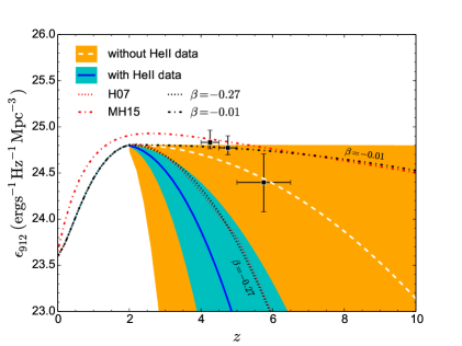
Figure 1: MCMC constraints on ionizing comoving AGN emissivity for two different cases: (i) without taking He $\scriptstyle\rm II$ data - white dashed lines for best-fit result with orange shaded region around it for 2-$\sigma$ C.L., (ii) with He $\scriptstyle\rm II$ data - solid blue curve for the best-fit with shaded cyan region for 2-$\sigma$ limits. The H07 (or $\beta=-0.27$) and MH15 (or $\beta=-0.01$) models are also shown here by dotted and dot-dashed curves respectively.The black points with errorbars are the observed data inferred from QLFs by Giallongo et al. (2015).

The results from our current MCMC analysis for these two models are summarized in Table 1, where the first four rows are for the free parameters of the model and the last one ($\tau_{\rm el}$) corresponds to the derived parameter. For comparison, we also show here H07 ($\beta=-0.27$) and MH15 ($\beta=-0.01$) cases. For that, we fix the $\Delta_{\rm crit}=60$ (following our earlier works) and choose some combination of $\epsilon_{\rm II}$ and $\lambda_{0}$ (without running the MCMC) so that they can reasonably match all the observed datasets for HI Ly$\alpha$ effective optical depth, redshift evolution of LLSs and also produce $\tau_{\rm el}$ which is allowed by Planck 2016. We have plotted the MCMC constraints on the comoving AGN emissivities in Fig. 1 and the other quantities of interest in Fig. 2. The constraints on the fraction of hydrogen photoionization rates contributed by QSOs (compared to its total, i.e., QSOs + galaxies, value) are shown in Fig. 3. For comparison, we also show the H07 and MH15 models in these three figures.

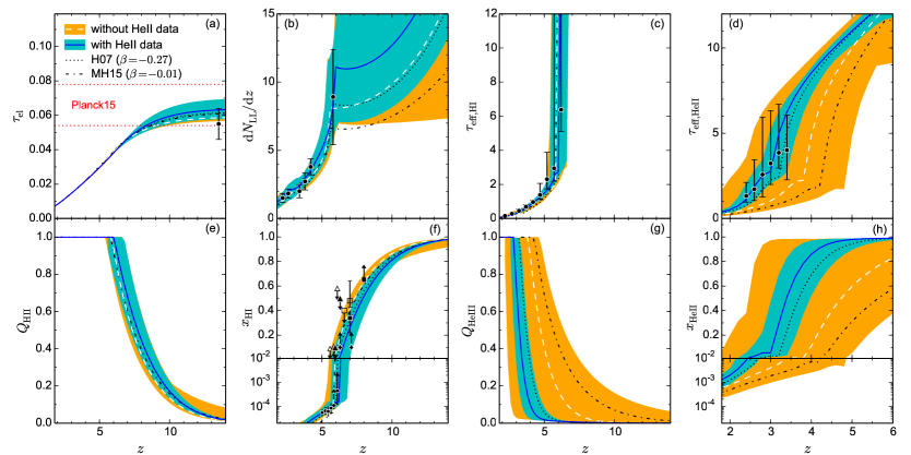
Figure 2: The MCMC constraints on various quantities related to reionization. Different panels indicate: (a) electron scattering optical depth $\tau_{\rm el}$, (b) redshift evolution of Lyman-limit systems ${\rm d}N_{\rm LL}/{\rm d}z$, (c) effective H $\scriptstyle\rm I$ Ly$\alpha$ optical depth $\tau_{\rm eff,HI}$, (d) effective He $\scriptstyle\rm II$ Ly$\alpha$ optical depth $\tau_{\rm eff,HeII}$, (e) volume filling factor of ionized hydrogen $Q_{\rm HII}$, (f) neutral hydrogen fraction $x_{\rm HI}(z)$, (g) He $\scriptstyle\rm III$ ionized volume filling factor $Q_{\rm HeIII}$ and (h) global He $\scriptstyle\rm II$ fraction $x_{\rm HeII}$. The solid blue and dashed white lines correspond to the mean evolution obtained from the models with He $\scriptstyle\rm II$ data and without He $\scriptstyle\rm II$ data respectively. The shaded regions refer to the 2-$\sigma$ confidence limits around the mean value of the corresponding models. The black points with errorbars are the current observational limits on reionization, see the main text for references. For comparison, we also plot the H07 (i.e. $\beta=-0.27$) and MH15 ($\beta=-0.01$) models.

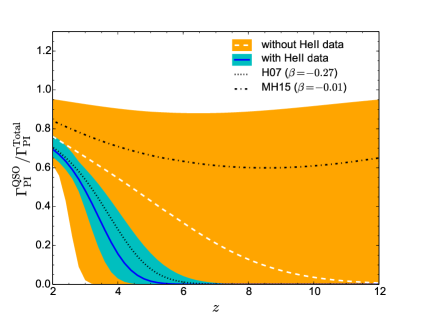
Figure 3: Same as Fig. 2, but showing the constraints on the ratio of photoionization rates coming from quasars to its total (galaxies + quasars) value at different redshifts.

3.1 Constraints “without He $\scriptstyle\rm II$ data”

The 2-$\sigma$ or 95% confidence limits on our model parameters without He $\scriptstyle\rm II$ data are given in the second column of Table 1 and shown by the shaded orange regions in Figs 1–3. The best-fit model is shown by the dashed white curves in these figures. We can see from the table that the data allows a wide range of $\beta$ values spanning from $\sim-4$ (signifying that the quasar contributions are almost negligible at $z>2$) to $\sim 0$ (signifying that the quasars dominate even at higher redshifts and a very little contribution is coming from galaxies). This is also evident from Fig. 1 where we see that the shaded orange region is remarkably wide. Both the H07 (dotted black curve) and MH15 (dot-dashed black curve) cases are well inside this allowed region at $z\gtrsim 4$.

From the MCMC constraints on various quantities related to reionization shown in Fig. 2, we find that the allowed 2-$\sigma$ confidence limits are relatively narrower for low-$z$ regime and increase at $z\gtrsim 6$. This is expected as most of the datasets used in this work exist only at low redshifts $z\leq 6$, whereas the higher-$z$ epoch is poorly constrained (Mitra et al., 2011, 2015). The reionization optical depth for the best-fit model is in a good agreement with the Planck 2016 data (black point with errorbar in panel a). We also show the earlier Planck 2015 limit by dotted red lines. In panel b, we plot the evolution of Lyman-limit systems which again matches he combined observational data points from Songaila & Cowie (2010) and Prochaska et al. (2010) at $2<z<6$ quite reasonably for the constraints obtained. We plot the evolution of effective optical depth of H $\scriptstyle\rm I$ Ly$\alpha$ absorption $\tau_{\rm eff,HI}$ in panel c. The MCMC constraint obtained is in general agreement with the observational measurements from Fan et al. (2006); Becker et al. (2013) in the interval $2<z<6$. From the evolution of volume filling factor $Q_{\rm HII}$ of H $\scriptstyle\rm II$ regions (panel e) and the global neutral hydrogen fraction $x_{\rm HI}$ (panel f), we find that the hydrogen reionization history is reasonably well constrained, in spite of the quasar emissivity being allowed to take such wide range of values. This is because any variation in $\beta$ is appropriately compensated by a similar change in $\epsilon_{\rm II}$ making sure that the models agree with the observations. In fact, the allowed range of $\epsilon_{\rm II}$, as can be seen from Table 1, is also quite wide between $\sim 4\times 10^{-4}-\sim 5\times 10^{-3}$. We also find that the model can match the current observed constraints on $x_{\rm HI}$ quite reasonably within their errorbars. Note that the match is quite impressive, given the fact that we did not include these datasets, except the McGreer et al. (2015) data at $z\sim 5-6$, as constraints in the current analysis. The observational limits (black points) are taken from various measurements by Fan et al. (2006) (filled circle), McGreer et al. (2015) (open triangle), Totani et al. (2006); Chornock et al. (2013) (filled triangle), Bolton et al. (2011); Schroeder et al. (2013) (filled diamond), Ota et al. (2008); Ouchi et al. (2010) (open square), Schenker et al. (2014) (filled square).

Moving on to quantities related to He $\scriptstyle\rm II$ reionization, we plot the effective optical depth $\tau_{\rm eff,HeII}$ in panel d. The points with error bars are from Worseck et al. (2016), binned appropriately for the MCMC analysis. Note that, these data points are not taken into account for the results presented in this subsection. Clearly, ignoring these data points leads to the 2-$\sigma$ allowed regions that are considerably wide which is also related to the fact that $\beta$ is allowed to take a wide range of values. We show the evolution of He $\scriptstyle\rm III$ ionized volume fraction $Q_{\rm HeIII}$ and the global He $\scriptstyle\rm II$ fraction $x_{\rm HeII}$ in panels g and h, respectively. The case $Q_{\rm HeIII}=1$ implies that helium is doubly reionized, and the $x_{\rm HeII}$ in that case is determined by the residual He $\scriptstyle\rm II$ fraction in the He $\scriptstyle\rm III$ regions. The global He $\scriptstyle\rm II$ reionization history mainly depends on the contribution from QSOs and thus leaves a distinguishing feature for different $\beta$ models - higher the value of $\beta$, earlier the He $\scriptstyle\rm II$ reionization occurs. The best-fit model without He $\scriptstyle\rm II$ data or the AGN-dominated MH15 model indicates that, the helium becomes doubly reionized at $z\gtrsim 4$, however, the 2-$\sigma$ limits allow a wide range of reionization redshifts. For example, He $\scriptstyle\rm II$ reionization is allowed to be completed as early as $z\sim 5$ (implying a high $\beta\sim 0$) and as late as $z\sim 2.5$ (implying a low $\beta\sim-4$).

From Fig. 3, we find that the fraction of the photoionization rate contributed by the quasars can take any value between $0$ and $\sim 90\%$ at $z>3$. Interestingly, the data allow the fraction to have consistently high value $\sim 90\%$ over the full redshift range $2<z<12$ considered here. These models would correspond to quasar dominated reionization scenarios which, as we can see, cannot be ruled out by hydrogen reionization data alone.

3.2 Constraints “with He $\scriptstyle\rm II$ data”

The constraints on the model parameters change significantly when we include the $\tau_{\rm eff,HeII}$ data in our analysis. The 2-$\sigma$ or 95% confidence limits on our model parameters with He $\scriptstyle\rm II$ data are given in the third column of Table 1 and shown by the shaded cyan regions in Figs 1–3. The solid blue curves in these figures correspond to the best-fit model. The values quoted in the table show that the confidence limits on $\beta$ and $\epsilon_{\rm II}$ are considerably shrunk when the He $\scriptstyle\rm II$ data are accounted for. The allowed values of $\beta$ are between $-0.99$ and $-0.19$, which accommodates the H07 ($\beta=-0.27$) model, but strongly disfavours the MH15 ($\beta=-0.01$) model. This can also be seen from Fig 1. In fact, the data now favours a considerably lower emissivity at $z\sim 4-5$ and is only marginally consistent with the value inferred from QLFs observation by Giallongo et al. (2015) (black points with errorbars).

One can see from Table 1 that, the constraints with He $\scriptstyle\rm II$ data require a significant contribution from the stars as reionization sources $\epsilon_{\rm II}\sim 0.003-0.005$ (2-$\sigma$ limits), which in turn corresponds to an escape fraction $\sim 8\%-13\%$ at $z\gtrsim 6$ of ionizing photons from galaxies. This is consistent with the results from our earlier work (Mitra et al., 2015), where we used the H07 model.

From the MCMC constraints shown in Fig. 2, we find, as expected, that the effect of including He $\scriptstyle\rm II$ data on quantities related to hydrogen reionization is negligible (panels a, b, c, e, f). The best-fit model with He $\scriptstyle\rm II$ data supports a slightly earlier hydrogen reionization epoch; mean $x_{\rm HI}$ goes from $\sim 0.8$ to $\sim 10^{-4}$ between $z=10.0$ and $z=6.2$. However, the constraints on He $\scriptstyle\rm II$ reionization are significantly different compared to the earlier case. This is solely driven by the $\tau_{\rm eff,HeII}$ data (panel d) which essentially disfavours a large set of models which were otherwise allowed by the hydrogen reionization datasets. We find that the best-fit effective He $\scriptstyle\rm II$ Ly$\alpha$ opacity increases rapidly from $z=2.4$ to $z=3.4$ by a factor of $\sim 6$. The data puts a tight constraint on the He $\scriptstyle\rm II$ reionization redshift between $2.5-3.5$, with the best-fit reionization redshift being $z=3$. The model agrees quite well with the interpretation of the He $\scriptstyle\rm II$ Ly$\alpha$ opacity data by Worseck et al. (2016) who suggested that helium is predominantly in the doubly ionized state in $\sim 50\%~{}(\sim 90\%)$ of the IGM at $z\simeq 3.4$ $(z\simeq 2.8)$. This should be compared with our predictions of the volume filling factor of He $\scriptstyle\rm III$ regions for the best-fit model which gives $Q_{\rm HeIII}\sim 50\%$ at $z\simeq 3.4$, remarkably consistent with that given by Worseck et al. (2016). The corresponding value at $z\simeq 2.8$ is $Q_{\rm HeIII}\sim 95\%$ for our model which is slightly higher than the Worseck et al. (2016) value, however, the two results are fully consistent if we account for the statistical uncertainties in our analysis. The H07 model also yields a very similar evolution as the best-fit blue curve. Models with $\beta<-1(\beta>-0.2)$ imply a very late (early) reionization history and fail to match observational data. However, an improved survey with much larger sample of $z>3$ He $\scriptstyle\rm II$ sightlines will be needed to put a tighter constraint on $\beta$ in future.

The fraction of photoionization rate contributed by the quasars, as shown in Fig 3, is significantly small. It can take values at most $\sim 10\%$ ($\sim 50\%$) at $z=6(4)$, thus implying that quasar dominated reionization models at $z>6$ are strongly disfavoured. For the best-fit model with He $\scriptstyle\rm II$ data and H07, the AGN contributions become negligible at $z\gtrsim 6$, which is in stark contrast against the MH15 case where the AGNs dominate ($\gtrsim 60\%$ of total value) even at higher redshifts.

As far as the other quantities are concerned, we find that the best-fit value of $\Delta_{\rm crit}$ is slightly larger for the model without He $\scriptstyle\rm II$ data, as it allows higher contribution from the QSOs than the model with He $\scriptstyle\rm II$ data. However, both the models support a much broader range for this parameter; $\Delta_{\rm crit}\sim 25-60$ within the 2-$\sigma$ limits. Thus, our results do not vary considerably for the choice of $\Delta_{\rm crit}$ as long as it is within this limit. We also find that, the electron scattering optical depths $\tau_{\rm el}$ for all the best-fit models are in good agreement with the Planck 2016 value. Interestingly, when we include He $\scriptstyle\rm II$ data, the best-fit model predicts slightly higher $\tau_{\rm el}$ than the other models, as it allows the highest stellar contributions among them.

Interestingly, we find that for the best-fit He $\scriptstyle\rm II$ model which is consistent with all the datasets considered in this paper, the stellar component of the comoving ionizing emissivity (in units of s^-1 Mpc^-3) can be fitted quite well by fitting functions of the form

$$\log\dot{n}_{\rm ion}^{\rm stellar}(z)=59.786~{}{\rm e}^{-0.008z}-9.844~{}{\rm e}^{-0.079z}$$ (6)

which, when combined with the QSO emissivities given in Section 2.1, should be useful in computing the reionization history.

4 Thermal evolution of IGM

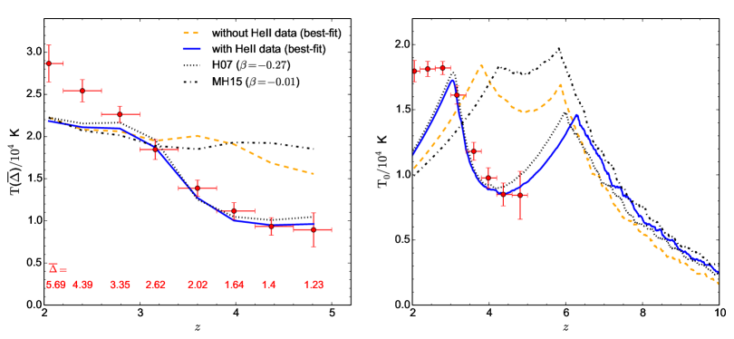
Figure 4: Thermal history for four different reionization models with different AGN emissivities; model with $\beta=-0.06$ (orange dashed), $\beta=-0.43$ (blue solid), $\beta=-0.27$ (black dotted) and $\beta=-0.01$ (black dot-dashed line). Left panel: evolution of IGM temperature at different overdensities printed at the bottom of the plot. The data points shown here are from the Ly$\alpha$ forest temperature measurements by Becker et al. (2011). Right panel: temperature of gas at mean IGM density ($\Delta=1$). Data points are inferred from the same temperature measurements, but corrected for the appropriate $\gamma$ (slope of the temperature-density relation) of our best-fit model with He $\scriptstyle\rm II$ data (solid blue lines).

A different way of constraining the quasar emissivity and the associated He $\scriptstyle\rm II$ reionization is by studying the thermal history of the IGM. The AGN-dominated models can lead to an additional heating of the IGM as they produce significantly more hard ionizing photons with energies in excess of 4 Ry compared to stellar sources. Thus the observational measurements on the IGM temperature can also be used to discriminate between different source models and put additional constraints on reionization (Zaldarriaga et al., 2001; Trac et al., 2008; Furlanetto & Oh, 2009; Cen et al., 2009; Raskutti et al., 2012; Padmanabhan et al., 2014).

Note that a careful calculation of the thermal evolution of the IGM is computationally much more expensive than that for the semi-analytic models described in the earlier sections and hence is not suitable for including in the MCMC analysis. Instead, we calculate the thermal histories for our best-fit models (along with the H07 and MH15 cases) and compare our predictions with the observations from Becker et al. (2011).

Our model computes the IGM temperature ($T$) evolution self-consistently and separately for each of the three regions, i.e., (i) completely neutral, (ii) regions where hydrogen is ionized and helium is singly ionized and (iii) where both species are fully ionized. For neutral regions, the temperature is usually assumed to decrease adiabatically while in the ionized regions, it is calculated as (Choudhury & Ferrara, 2005; Upton Sanderbeck et al., 2016):

$$\frac{{\rm d}T}{{\rm d}t} = -2H(t)T+\frac{2}{3}\frac{T}{\Delta}\frac{{\rm d}\Delta}{{\rm d}t}$$ (7)

$$-\frac{T}{\sum_{i}X_{i}}\frac{{\rm d}}{{\rm d}t}\sum_{i}X_{i}+\frac{2}{3k_{B}n_{b}(1+z)^{3}}\frac{{\rm d}E}{{\rm d}t}$$

where we have defined

$$X_{i}\equiv\frac{n_{i}m_{p}}{\overline{\rho}_{b}(\Delta)}$$ (8)

for three independent species $X_{\rm HI}$, $X_{\rm HeI}$, $X_{\rm HeIII}$ and $\overline{\rho}_{b}$ is the proper mass density of baryons. The first term on the right-hand side accounts for the adiabatic cooling of gas due to cosmic expansion. The second term calculates the adiabatic evolution due to collapsing overdensities. The third term describes the rate of change in the number of particles of the system and in the last term on the right-hand side, ${\rm d}E/{\rm d}t$ represents the net heating rate per baryon which encodes all other possible heating and cooling processes. For most purposes, it is sufficient to take into account only the photoheating, recombination cooling and Compton cooling off CMB photons (Choudhury & Ferrara, 2005).

In order to calculate the temperature at a given density ${\rm\Delta}$ and redshift $z$, we track the thermal evolution of a large number of density elements ($\sim 50,000$), generated according to the IGM probability distribution. It is this step which increases the computational cost of the analysis. During hydrogen reionization, our model assumes that all regions with $\Delta>\Delta_{\rm crit}$ remain neutral, while a fraction $Q_{\rm HII}$ of $\Delta<\Delta_{\rm crit}$ regions are ionized (Miralda-Escudé et al., 2000). In the post-reionization $Q_{\rm HII}=1$ era, the effect of ionizing radiation is to increase the value of the density threshold above which the IGM is neutral. At every time step, we calculate the increase in the ionized fraction and randomly assign the corresponding number of density elements as newly ionized. Following Upton Sanderbeck et al. (2016) and D’Aloisio et al. (2017) (and the references therein), each of these density elements is instantaneously heated, on top of the uniform photoheating background, to a temperature of $20,000$ K. We follow an identical procedure for He $\scriptstyle\rm II$ reionization as well and assume the density elements to be additionally heated by $8,000$ K when they reach their He $\scriptstyle\rm II$ reionization redshifts.

This method allows us to calculate, at any given redshift, the dependence of the gas temperature $T(\Delta)$ on the overdensity $\Delta$. We can fit the $T(\Delta)$ relation using a power-law of the form

$$T(\Delta)=T_{0}~{}\Delta^{\gamma-1},$$ (9)

where $T_{0}$ is the temperature of the mean density ($\Delta=1$) gas and $\gamma$ is the slope of the temperature-density relation. We can estimate the values of $T_{0}$ and $\gamma$ at every redshift.

In the left panel of Fig. 4, we show the redshift evolution of IGM temperature $T(\overline{\Delta})$ at different overdensities $\overline{\Delta}$ at redshifts where the data points from Becker et al. (2011) exist. Different curves are for different quasar emissivity models, while the points with error bars are the observed data (Becker et al., 2011). The first point to note is that all the models, irrespective of their quasar emissivity, underpredict the temperature at $z<3$. This could be because of assumptions in our semi-analytic model (e.g., the effective spectral index of the radiation from the quasars could be harder than what we assumed, which would lead to additional heating), or because of additional heating sources like the blazars (Puchwein et al., 2012), cosmic rays or intergalactic dust absorption (Upton Sanderbeck et al., 2016). Given the fact that our calculations of the temperature do not match the observations at $z<3$, any conclusions drawn in this section should be interpreted with caution.

We find that the H07 model and our best-fit model with He $\scriptstyle\rm II$ data are in excellent agreement with the observations at $z\gtrsim 3$. On the other hand, models with a more quasar contribution, i.e., the MH15 and the best-fit model without He $\scriptstyle\rm II$ data, predict considerably higher temperature than what is observed at these redshifts. These models have considerably earlier He $\scriptstyle\rm II$ reionization and hence the IGM is significantly photoheated at $3\lesssim z\lesssim 5$.

The same trends can be seen from the evolution of temperature at the mean density $T_{0}(z)$ (right panel). The two peaks seen in all the models correspond to the hydrogen and He $\scriptstyle\rm II$ reionization respectively. Also shown are the data points from the same observation by Becker et al. (2011), but adjusted accordingly using the temperature-density relation of the best-fit model with He $\scriptstyle\rm II$ data (solid blue lines). Models with higher $\beta$ heat up the IGM at much earlier epoch than the what the observations show. Our main findings are in excellent agreement with the recent study by D’Aloisio et al. (2017), where they conclude that the AGN-dominated scenario struggles to match the temperature measurements.

5 Conclusions

The new Planck results along with the recent discovery of significantly high number of faint AGNs from multiwavelength deep surveys at higher redshifts (Fiore et al., 2012; Giallongo et al., 2015) demand careful investigation of the actual contribution from star-forming galaxies and quasars as reionization sources. In addition, various current studies suggest that the globally-averaged escape fraction of ionizing photons is very small $\sim$ a few percent (Madau & Dickinson, 2014; Ma et al., 2015; Mitra et al., 2015; Hassan et al., 2016). Based on this idea, a QSO dominated reionization scenario has been explored in many contemporary studies (Madau & Haardt, 2015; Khaire et al., 2016; Yoshiura et al., 2016). On the other hand, Kim et al. (2015) and Jiang et al. (2016) claimed that the number of spectroscopically identified faint AGNs may not be high enough to fully account for the reionization of the IGM. Recently, D’Aloisio et al. (2017) also indicates a possible drawback of such high AGN emissivity models. This makes the claim of quasar-dominated scenario debatable. Thus, it would be interesting to see how our data-constrained semi-analytical reionization model can distinguish between the models with different comoving AGN emissivities. In this work, we have expanded our previous model (Mitra et al., 2015) and evaluated the impact of QSOs on reionization for different cases. As the observations on AGN emissivities at $z>3$ are still very uncertain, we model the AGN contribution in a way that its evolution at high redshifts ($z>2$) will solely be determined by a single parameter $\beta$. We check that, $\beta=-0.27$ and $\beta=-0.01$ can reasonably restore our old model with the observed quasar luminosity functions from Hopkins et al. (2007) and a quasar-dominated model with best-fit AGN emissivity from Madau & Haardt (2015) respectively. We denote the former case as H07 and the later one as MH15. We try to constrain the value of $\beta$ against different observations related to hydrogen and helium reionization: measurements of effective H $\scriptstyle\rm I$ Ly$\alpha$ optical depth $\tau_{\rm eff,HI}$, redshift evolution of LLS ${\rm d}N_{\rm LL}/{\rm d}z$, reionization optical depth from Planck 2016 and He $\scriptstyle\rm II$ Ly$\alpha$ forest data.

• We find that if we do not include He $\scriptstyle\rm II$ data in our analysis, a wide range of $\beta$-model can be allowed by the current observations. Both the quasar-dominated ($\beta\sim 0$) and stellar-dominated ($\beta\sim-4$; negligible QSOs at $z>2$) scenarios are possible within the 2-$\sigma$ confidence limits. Any variation in the quasar emissivity is appropriately compensated by the radiation from the stellar sources, thus ensuring that the constraints arising from hydrogen reionization data are not violated. It is thus not possible to put any meaningful constraints on the quasar emissivity using hydrogen reionization alone.

• In contrast, using He $\scriptstyle\rm II$ data in the analysis can put a tighter constraint on $\beta$ and rules out the possibility of quasar dominated models of hydrogen reionization. This model supports the decade-old two-component view of cosmic reionization; quasars contribute significantly at lower redshifts and later the star-forming early galaxies take over. An escape fraction of $8$ to $13\%$ from those galaxies at $z\gtrsim 6$ are needed to provide the appropriate ionizing flux. The fraction of photoionization rate contributed by the quasars cannot be larger that $\sim 10\%(\sim 50\%)$ at $z=6(4)$.

• The models where AGNs throughout dominate the reionization process (e.g. MH15 model) favour an early helium reionization (completed at $z\gtrsim 4$) history. They produce a much more slowly evolving He $\scriptstyle\rm II$ effective optical depth than observation (Worseck et al., 2016) suggests. Also such models are inconsistent with the observational measurements of IGM temperature (Becker et al., 2011). They heat up the IGM at much earlier epoch than the actual observation indicates.

• On the other hand, the model constrained by He $\scriptstyle\rm II$ data has no difficulties in matching both the $\tau_{\rm eff,HeII}$ and temperature data. The best-fit model predicts a relatively late helium reionization ending at $z\approx 3$. $\tau_{\rm eff,HeII}$ increases rapidly from $z=2.4$ to $z=3.4$ by a factor of $\sim 6$. Our old H07 case is well within the 2-$\sigma$ limits of such models.

As a final note, we should mention some caveats of our model. The star-formation efficiency and escape fraction parameters should depend on the halo mass and/or redshifts (however weakly). For simplicity, we take them as a constant throughout this work. A detailed probe of parameter space using the principal component analysis, at the expense of larger computational time, might be useful in this case. We notice that, our simplified $\lambda_{\rm mfp}$ prescription starts to break down when it becomes comparable to the Hubble radius at low-redshift regime ($z\lesssim 2$). Perhaps a more accurate mean free path calculation will be needful. In our model, following Miralda-Escudé et al. (2000), we assume that reionization is said to be complete once all the low-density regions with $\Delta<\Delta_{\rm crit}$ are ionized, while the higher density gas is still neutral. This postulate might not be fully correct, as in a real scenario, the ionization factor can depend on the local intensity of ionizing photons and/or the degree of self-shielding (Miralda-Escudé et al., 2000; Choudhury, 2009). Furthermore, a proper account of the quasar proximity effect (where the ionization rate around a quasar exceeds the background flux) in our model might provide additional insights (Bajtlik et al., 1988; Miralda-Escudé & Rees, 1994; Padmanabhan et al., 2014; D’Aloisio et al., 2017). Finally, recent observations (Becker et al., 2015) indicate a rapid dispersion in Ly-$\alpha$ forest effective optical depth at $z>5$. D’Aloisio et al. (2016) argued that matching such large scatter requires a much shorter (factor of $\gtrsim 3$) spatially averaged mean free path than the actual measured value from Worseck et al. (2014) at high redshifts, assuming galaxies to be the dominant sources of ionizing photons (Davies & Furlanetto, 2016). However, they also claimed that these opacity fluctuations might be driven by the residual inhomogeneities in the IGM temperature arising from a patchy reionization process rather than by the ionization background itself. A more rigorous modeling of IGM along with a careful estimation of mean free path is needed in our analysis to fully include these effects. Also, our model for temperature evolution is probably not very accurate at low redshifts ($z<3$). Additional sources of heating like blazars might also be required, which we have not considered in this work.

Nonetheless, future discovery of faint quasars at high redshifts might be worthwhile to clearly distinguish between the models with different AGN contribution. A refined reionization model along with the improved measurements on intergalactic He $\scriptstyle\rm II$ Ly$\alpha$ absorption spectra and high-redshift temperature measurements will be needed to put a more decisive constraint on the helium reionization scenario.

References

- Bajtlik et al. (1988) Bajtlik S., Duncan R. C., Ostriker J. P., 1988, ApJ, 327, 570
- Barkana & Loeb (2001) Barkana R., Loeb A., 2001, Phys. Rep., 349, 125
- Becker & Bolton (2013) Becker G. D., Bolton J. S., 2013, MNRAS, 436, 1023
- Becker et al. (2001) Becker R. H., et al., 2001, Astron.J., 122, 2850
- Becker et al. (2011) Becker G. D., Bolton J. S., Haehnelt M. G., Sargent W. L. W., 2011, MNRAS, 410, 1096
- Becker et al. (2013) Becker G. D., Hewett P. C., Worseck G., Prochaska J. X., 2013, MNRAS, 430, 2067
- Becker et al. (2015) Becker G. D., Bolton J. S., Madau P., Pettini M., Ryan-Weber E. V., Venemans B. P., 2015, MNRAS, 447, 3402
- Bennett et al. (2013) Bennett C. L., et al., 2013, ApJS, 208, 20
- Bolton & Haehnelt (2007) Bolton J. S., Haehnelt M. G., 2007, MNRAS, 382, 325
- Bolton et al. (2011) Bolton J. S., et al., 2011, MNRAS, 416, L70
- Bouwens & Illingworth (2006) Bouwens R., Illingworth G., 2006, New Astronomy Reviews, 50, 152
- Bouwens et al. (2015a) Bouwens R. J., et al., 2015a, ApJ, 803, 34
- Bouwens et al. (2015b) Bouwens R. J., Illingworth G. D., Oesch P. A., Caruana J., Holwerda B., Smit R., Wilkins S., 2015b, ApJ, 811, 140
- Bowler et al. (2014) Bowler R. A. A., et al., 2014, arXiv:1411.2976,
- Bradley et al. (2012) Bradley L. D., et al., 2012, ApJ, 760, 108
- Cai et al. (2014) Cai Z.-Y., Lapi A., Bressan A., De Zotti G., Negrello M., Danese L., 2014, ApJ, 785, 65
- Cen et al. (2009) Cen R., McDonald P., Trac H., Loeb A., 2009, ApJL, 706, L164
- Chornock et al. (2013) Chornock R., et al., 2013, ApJ, 774, 26
- Choudhury (2009) Choudhury T. R., 2009, Current Science, 97, 841
- Choudhury & Ferrara (2005) Choudhury T. R., Ferrara A., 2005, MNRAS, 361, 577
- Choudhury & Ferrara (2006a) Choudhury T. R., Ferrara A., 2006a, preprint, (arXiv:astro-ph/0603149)
- Choudhury & Ferrara (2006b) Choudhury T. R., Ferrara A., 2006b, MNRAS, 371, L55
- Choudhury et al. (2014) Choudhury T. R., Puchwein E., Haehnelt M. G., Bolton J. S., 2014, arXiv:1412.4790,
- Civano et al. (2011) Civano F., et al., 2011, ApJ, 741, 91
- Compostella et al. (2013) Compostella M., Cantalupo S., Porciani C., 2013, MNRAS, 435, 3169
- Compostella et al. (2014) Compostella M., Cantalupo S., Porciani C., 2014, MNRAS, 445, 4186
- D’Aloisio et al. (2016) D’Aloisio A., McQuinn M., Davies F. B., Furlanetto S. R., 2016, preprint, (arXiv:1611.02711)
- D’Aloisio et al. (2017) D’Aloisio A., Upton Sanderbeck P. R., McQuinn M., Trac H., Shapiro P. R., 2017, MNRAS, 468, 4691
- Davies & Furlanetto (2016) Davies F. B., Furlanetto S. R., 2016, MNRAS, 460, 1328
- Dijkstra et al. (2007) Dijkstra M., Wyithe J. S. B., Haiman Z., 2007, MNRAS, 379, 253
- Dixon & Furlanetto (2009) Dixon K. L., Furlanetto S. R., 2009, ApJ, 706, 970
- Fan et al. (2006) Fan X., et al., 2006, AJ, 132, 117
- Faucher-Giguère et al. (2009) Faucher-Giguère C.-A., Lidz A., Zaldarriaga M., Hernquist L., 2009, ApJ, 703, 1416
- Finlator et al. (2016) Finlator K., Oppenheimer B. D., Davé R., Zackrisson E., Thompson R., Huang S., 2016, MNRAS, 459, 2299
- Fiore et al. (2012) Fiore F., et al., 2012, A&A, 537, A16
- Furlanetto & Oh (2009) Furlanetto S. R., Oh S. P., 2009, ApJ, 701, 94
- Gallerani et al. (2006) Gallerani S., Choudhury T. R., Ferrara A., 2006, MNRAS, 370, 1401
- Giallongo et al. (2012) Giallongo E., Menci N., Fiore F., Castellano M., Fontana A., Grazian A., Pentericci L., 2012, ApJ, 755, 124
- Giallongo et al. (2015) Giallongo E., et al., 2015, A&A, 578, A83
- Gleser et al. (2005) Gleser L., Nusser A., Benson A. J., Ohno H., Sugiyama N., 2005, MNRAS, 361, 1399
- Glikman et al. (2011) Glikman E., Djorgovski S. G., Stern D., Dey A., Jannuzi B. T., Lee K.-S., 2011, ApJL, 728, L26
- Hassan et al. (2016) Hassan S., Davé R., Finlator K., Santos M. G., 2016, MNRAS, 457, 1550
- Hopkins et al. (2007) Hopkins P. F., Richards G. T., Hernquist L., 2007, ApJ, 654, 731
- Iliev et al. (2008) Iliev I. T., Shapiro P. R., McDonald P., Mellema G., Pen U.-L., 2008, MNRAS, 391, 63
- Jiang et al. (2016) Jiang L., et al., 2016, ApJ, 833, 222
- Khaire & Srianand (2013) Khaire V., Srianand R., 2013, MNRAS, 431, L53
- Khaire et al. (2016) Khaire V., Srianand R., Choudhury T. R., Gaikwad P., 2016, MNRAS, 457, 4051
- Kim et al. (2015) Kim Y., et al., 2015, ApJL, 813, L35
- Komatsu et al. (2011) Komatsu E., et al., 2011, Astrophys.J.Suppl., 192, 18
- Kulkarni & Choudhury (2011) Kulkarni G., Choudhury T. R., 2011, MNRAS, 412, 2781
- Lewis & Bridle (2002) Lewis A., Bridle S., 2002, Phys. Rev. D, 66, 103511
- Loeb (2006) Loeb A., 2006, preprint, (arXiv:astro-ph/0603360)
- Loeb & Barkana (2001) Loeb A., Barkana R., 2001, ARA&A, 39, 19
- Ma et al. (2015) Ma X., Kasen D., Hopkins P. F., Faucher-Giguère C.-A., Quataert E., Kereš D., Murray N., 2015, MNRAS, 453, 960
- Madau & Dickinson (2014) Madau P., Dickinson M., 2014, ARA&A, 52, 415
- Madau & Haardt (2015) Madau P., Haardt F., 2015, ApJL, 813, L8
- McGreer et al. (2015) McGreer I. D., Mesinger A., D’Odorico V., 2015, MNRAS, 447, 499
- McLeod et al. (2014) McLeod D. J., McLure R. J., Dunlop J. S., Robertson B. E., Ellis R. S., Targett T. T., 2014, arXiv:1412.1472,
- McQuinn (2016) McQuinn M., 2016, ARA&A, 54, 313
- McQuinn et al. (2009) McQuinn M., Lidz A., Zaldarriaga M., Hernquist L., Hopkins P. F., Dutta S., Faucher-Giguère C.-A., 2009, ApJ, 694, 842
- Mesinger et al. (2015) Mesinger A., Aykutalp A., Vanzella E., Pentericci L., Ferrara A., Dijkstra M., 2015, MNRAS, 446, 566
- Miralda-Escudé & Rees (1994) Miralda-Escudé J., Rees M. J., 1994, MNRAS, 266, 343
- Miralda-Escudé et al. (2000) Miralda-Escudé J., Haehnelt M., Rees M. J., 2000, ApJ, 530, 1
- Mitra et al. (2011) Mitra S., Choudhury T. R., Ferrara A., 2011, MNRAS, 413, 1569
- Mitra et al. (2012) Mitra S., Choudhury T. R., Ferrara A., 2012, MNRAS, 419, 1480
- Mitra et al. (2013) Mitra S., Ferrara A., Choudhury T. R., 2013, MNRAS, 428, L1
- Mitra et al. (2015) Mitra S., Choudhury T. R., Ferrara A., 2015, MNRAS, 454, L76
- Oesch et al. (2012) Oesch P. A., et al., 2012, ApJ, 745, 110
- Oesch et al. (2014) Oesch P. A., et al., 2014, ApJ, 786, 108
- Okamoto et al. (2008) Okamoto T., Gao L., Theuns T., 2008, MNRAS, 390, 920
- Ota et al. (2008) Ota K., et al., 2008, ApJ, 677, 12
- Ouchi et al. (2010) Ouchi M., et al., 2010, ApJ, 723, 869
- Padmanabhan et al. (2014) Padmanabhan H., Choudhury T. R., Srianand R., 2014, MNRAS, 443, 3761
- Planck Collaboration et al. (2014) Planck Collaboration et al., 2014, A&A, 571, A16
- Planck Collaboration et al. (2016a) Planck Collaboration et al., 2016a, A&A, 594, A13
- Planck Collaboration et al. (2016b) Planck Collaboration et al., 2016b, A&A, 596, A107
- Planck Collaboration et al. (2016c) Planck Collaboration et al., 2016c, A&A, 596, A108
- Price et al. (2016) Price L. C., Trac H., Cen R., 2016, preprint, (arXiv:1605.03970)
- Prochaska et al. (2010) Prochaska J. X., O’Meara J. M., Worseck G., 2010, ApJ, 718, 392
- Puchwein et al. (2012) Puchwein E., Pfrommer C., Springel V., Broderick A. E., Chang P., 2012, MNRAS, 423, 149
- Raskutti et al. (2012) Raskutti S., Bolton J. S., Wyithe J. S. B., Becker G. D., 2012, MNRAS, 421, 1969
- Richards et al. (2006) Richards G. T., et al., 2006, ApJS, 166, 470
- Robertson et al. (2015) Robertson B. E., Ellis R. S., Furlanetto S. R., Dunlop J. S., 2015, ApJL, 802, L19
- Samui et al. (2007) Samui S., Srianand R., Subramanian K., 2007, MNRAS, 377, 285
- Schenker et al. (2014) Schenker M. A., Ellis R. S., Konidaris N. P., Stark D. P., 2014, ApJ, 795, 20
- Schirber & Bullock (2003) Schirber M., Bullock J. S., 2003, ApJ, 584, 110
- Schroeder et al. (2013) Schroeder J., Mesinger A., Haiman Z., 2013, MNRAS, 428, 3058
- Sharma et al. (2016) Sharma M., Theuns T., Frenk C., Bower R., Crain R., Schaller M., Schaye J., 2016, MNRAS, 458, L94
- Sobacchi & Mesinger (2013) Sobacchi E., Mesinger A., 2013, MNRAS, 432, 3340
- Songaila & Cowie (2010) Songaila A., Cowie L. L., 2010, ApJ, 721, 1448
- Totani et al. (2006) Totani T., et al., 2006, Pub. Astron. Soc. Japan, 58, 485
- Trac et al. (2008) Trac H., Cen R., Loeb A., 2008, ApJL, 689, L81
- Upton Sanderbeck et al. (2016) Upton Sanderbeck P. R., D’Aloisio A., McQuinn M. J., 2016, MNRAS, 460, 1885
- White et al. (2003) White R. L., Becker R. H., Fan X., Strauss M. A., 2003, AJ, 126, 1
- Worseck et al. (2014) Worseck G., et al., 2014, MNRAS, 445, 1745
- Worseck et al. (2016) Worseck G., Prochaska J. X., Hennawi J. F., McQuinn M., 2016, ApJ, 825, 144
- Wyithe & Loeb (2003) Wyithe J. S. B., Loeb A., 2003, ApJ, 586, 693
- Wyithe & Loeb (2005) Wyithe J. S. B., Loeb A., 2005, ApJ, 625, 1
- Yoshiura et al. (2016) Yoshiura S., Hasegawa K., Ichiki K., Tashiro H., Shimabukuro H., Takahashi K., 2016, preprint, (arXiv:1602.04407)
- Zaldarriaga et al. (2001) Zaldarriaga M., Hui L., Tegmark M., 2001, ApJ, 557, 519