Criteria For Superfluid Instabilities of Geometries
with Hyperscaling Violation

Abstract

We examine the onset of superfluid instabilities for geometries that exhibit hyperscaling violation and Lifshitz-like scaling at infrared and intermediate energy scales, and approach AdS in the ultraviolet. In particular, we are interested in the role of a non-trivial coupling between the neutral scalar supporting the scaling regime, and the (charged) complex scalar which condenses. The analysis focuses exclusively on unstable modes arising from the hyperscaling-violating portion of the geometry. Working at zero temperature, we identify simple analytical criteria for the presence of scalar instabilities, and discuss under which conditions a minimal charge will be needed to trigger a transition. Finite temperature examples are constructed numerically for a few illustrative cases.

I Introduction and Summary of Results

The recent efforts to use holography to probe strongly coupled quantum systems have led to new insights into the possible instabilities of a variety of gravitational solutions. One of the prime examples is that of charged black holes in Anti de Sitter (AdS) space, which have been understood to be unstable to the formation of scalar hair – thanks to attempts to realize the spontaneous breaking of an abelian gauge symmetry in gravity Gubser:2008px , and develop a holographic description of superconducting phases Hartnoll:2008vx ; Hartnoll:2008kx . For reviews of holographic superconductors we refer the reader to e.g. Hartnoll:2009sz ; Herzog:2009xv ; Horowitz:2010gk ; Cai:2015cya . Other notable examples include the spontaneous breaking of translational invariance and the onset of spatially modulated instabilities, which have been identified in a number of geometries (see Domokos:2007kt ; Nakamura:2009tf ; Ooguri:2010xs ; Donos:2011bh ; Bergman:2011rf for some of the early papers) and have potential applications to e.g. QCD and condensed matter systems with striped phases. We have seen growing interest in constructing gravitational solutions that exhibit a variety of broken symmetries, with significant attention recently given to realizing holographic lattices through the (explicit) breaking of translational invariance (see e.g. Hartnoll:2012rj ; Horowitz:2012ky ; Donos:2012js ; Vegh:2013sk ; Blake:2013bqa ; Donos:2013eha ; Andrade:2013gsa ; Gouteraux:2014hca ; Donos:2014oha ).

In this paper we revisit the question of scalar field instabilities associated with geometries that exhibit hyperscaling violation $\theta$ and non-relativistic scaling $z$, with the ultimate goal of reaching a more complete understanding of low temperature superconducting phase transitions in the dual systems. We will work with gravitational solutions which are hyperscaling violating and Lifshitz-like at infrared (IR) and intermediate energies, and asymptote to AdS in the ultraviolet (UV). Such geometries are well known to arise in Einstein-Maxwell-dilaton theories, and are supported by a neutral scalar subject to a rather simple potential. We require AdS asymptotics to ensure that the dual field theory is conformal at the UV fixed point – so that the violation of hyperscaling and relativistic symmetry is generated at lower energies – and thus can rely on the standard holographic dictionary. We stress that we are only interested in phase transitions that are triggered in the hyperscaling violating regime itself, since in full generality they are much less understood than their AdS counterpart.

Charged scalar field condensation on non-relativistic backgrounds that don’t respect hyperscaling has been studied in a number of settings (see e.g. Salvio:2013jia ; Fan:2013tga ; Lucas:2014sba but the list is by no means exhaustive), although typically for specific values of the scaling exponents $z$ and $\theta$ or in somewhat simple models. Here we will extend these analyses by introducing a non-trivial coupling of the form $\sim B(\phi)\,|\Psi|^{2}$ between the neutral scalar $\phi$ that determines the background and the charged scalar $\Psi$ that condenses. We will obtain analytical instability criteria – attempting to be generic, to the extent that it is possible – and highlight the role of $B(\phi)$ on the onset of the superfluid phase transition. Since $B(\phi)$ contributes to the effective mass of the charged scalar, it is intuitively clear that it will affect the condensation process – enhancing it or impeding it depending on its sign and its radial profile. Throughout the paper we will adopt the choice $B(\phi)\sim e^{\hat{\tau}\phi}$ in the hyperscaling violating regime, with $\hat{\tau}$ an arbitrary constant.

To probe the onset of the formation of scalar hair, we are going to focus on the linearized perturbation of the charged scalar $\Psi$ around the unbroken phase. To obtain the linearized equation of motion for $\Psi$ it suffices to know the structure of the charged scalar couplings up to quadratic order – such leading terms are enough to compute the temperature at which the unbroken phase becomes unstable to scalar hair. One should keep in mind, however, that the nonlinear details of the couplings could affect the order of the phase transition and the thermodynamics, as has been stressed in Kiritsis:2015hoa .

Our instability analysis will be done in two complementary ways. After setting up the model and the background in Sections II and III, we will inspect the behavior of the effective mass $M_{eff}^{2}$ of the charged scalar in Section IV, and in particular, the conditions under which it becomes sufficiently negative. In Section V we will then recast the linearized perturbation of the charged scalar in Schrödinger form, and perform a more detailed instability analysis by examining whether the effective Schrödinger potential $V_{Schr}$ is sufficiently negative to support bound states (for studies of instabilities in terms of an effective Schrödinger potential see e.g. Kodama:2003kk ; Hartnoll:2008kx ; Keeler:2013msa ). To complement the intuition developed from examining $M_{eff}^{2}$ and $V_{Schr}$, one should also analyze the structure of IR perturbations of the charged scalar, to ensure that they can indeed support a scalar condensate. As we will see, this can rule out regions of parameter space for which $M_{eff}^{2}$ and $V_{Schr}$ may be ambiguous. For simplicity, our analytical arguments are developed working at zero temperature, and are meant to serve as guidance for a more detailed finite temperature analysis. Still, we believe that they capture all the essential physics of their low temperature counterpart, as we confirm in our numerical section VI, in a few illustrative cases. We leave a more thorough finite temperature analysis to future work.

We will find many similarities with the standard holographic superconductor setup, but also some crucial differences. As in Gubser:2008px ; Hartnoll:2008vx ; Hartnoll:2008kx , two distinct mechanisms can lead to the condensation of a scalar in these background geometries. The gauge field contribution to the effective mass $M^{2}_{eff}$ of $\Psi$ is always negative and can become large enough to make it energetically favorable for the system to undergo a superfluid phase transition. Similarly, a negative coupling $B(\phi)$ can drive $M_{eff}^{2}$ to become appreciably negative, thus facilitating the transition. Since the latter process can happen even at zero charge, it allows neutral scalars to condense – and it is of course the analog of violating BF bounds in AdS.

What is novel in the models we consider here is the rich behavior associated with the possible profiles of the coupling $B(\phi)$, and its effect on the interplay between the two instability mechanisms. In particular, the condensation process is highly sensitive to the specific way in which $B(\phi)$ scales as compared to the $\{z,\theta\}$ background geometry – qualitatively new behavior will be seen when the effective mass term $B(\phi)\,\psi^{2}$ does not respect the scaling of the charged scalar kinetic term (here $\psi$ denotes the modulus of the complex scalar $\Psi$). We should note that the role of a coupling $\sim B(\phi)\psi^{2}$ in hyperscaling violating backgrounds was already discussed by Lucas:2014sba , although in a slightly different context. Choosing the coupling so that $B(\phi)\psi^{2}$ scales as $\sim(\partial\psi)^{2}$, the authors noted the presence of a minimal charge needed to form a condensate, and raised the question of whether it could be a universal feature. Here we will address this point working with general classes of $\{z,\theta\}$ geometries and couplings $B(\phi)\sim e^{\hat{\tau}\phi}$, and show that this is not generally the case – there is a somewhat large parameter space where neutral scalars can condense. We will also identify the cases in which we expect to see a minimal charge. As we will see, the existence of the latter will be sensitive to the detailed behavior of $B(\phi)$. Again, we find some crucial differences with the standard holographic superconductor setup, that can be traced to the non-trivial scaling properties of the coupling $B$ and the background itself.

I.1 Summary of Results

We work with the Lagrangian given in (5), so that the dual field theory has $d$ spatial dimensions. To respect the scaling of the potential $V(\phi)\propto e^{-\beta\phi}$ and gauge kinetic function $Z(\phi)\propto e^{\,\alpha\phi}$ of the hyperscaling violating background, we have taken the coupling between the two scalars to be of the form $B(\phi)\sim e^{\hat{\tau}\phi}$ or, in terms of the holographic radial coordinate $r$,

$$B(r)=B_{0}\,r^{\tau}\,,$$ (1)

with $\tau$ an arbitrary constant.

Our analytical estimates for the onset of scalar field instabilities are extracted first in Section IV by inspecting the effective mass for the charged scalar

$$M_{eff}^{2}(r)=\tilde{L}^{2}\left[B_{0}\,r^{\tau-2(m-1)}-Q^{2}r^{2dn}\right]+\Bigl{(}m+\frac{1}{2}dn\Bigr{)}\Bigl{(}m+\frac{1}{2}dn-1\Bigr{)}\,,$$ (2)

and then in Section V by examining when the effective Schrödinger potential

$$V_{Schr}(r)=r^{2(2m-1)}\left[B_{0}\,r^{\tau-2(m-1)}-Q^{2}r^{2dn}+\frac{1}{4\tilde{L}^{2}}\,dn\Bigl{(}dn+4m-2\Bigr{)}\right]$$ (3)

develops negative regions which can support the existence of bound states. Here $Q$ is proportional to the charge of $\Psi$, $\tilde{L}$ is a length scale defined in the main text and the parameters $\{m,n\}$ are

$$m=\frac{zd-\theta}{zd-2\theta}\,,\qquad n=\frac{d-\theta}{zd-2\theta}\,.$$ (4)

With our choice of coordinates the IR is located at $r=0$, while $r=r_{tr}$ will denote the transition scale between the non-relativistic, hyperscaling violating solution and the UV AdS region.

The possible sources of instability are now apparent. Superfluid phase transitions are generically triggered by a sufficiently large charge term $\propto Q^{2}$, driving $M_{eff}$ imaginary and $V_{Schr}$ negative. A negative and suitably large contribution from the coupling $\propto B_{0}$ will have the same effect, and is responsible for the formation of a condensate even when $Q=0$. Moreover, the interplay between the two terms can lead to interesting behaviors, depending on how $\tau$ compares to the exponents $m$ and $n$. While these expressions were obtained at zero temperature, they are expected to capture the key aspects of the finite temperature behavior. This is shown for a few illustrative cases in Section VI.

The main features that have emerged from this analysis are the following:

• In these hyperscaling violating backgrounds the gauge field term $\sim Q^{2}r^{2dn}$ always decreases towards to IR (as $r\rightarrow 0$), since $n>0$, as discussed in the main text.

• The competition between the contributions coming from the $U(1)$ gauge field and the real neutral scalar is very sensitive to the way in which $B(\phi)$ scales compared to the background, in particular to whether $\tau$ is larger or smaller than $2(m-1)$.

• Simplifications occur for the scaling choice $\tau=2(m-1)$, which corresponds to the coupling $B(\phi)\psi^{2}$ scaling in the same way as the kinetic term $(\partial\psi)^{2}$. In this case the only radial dependence of $M_{eff}^{2}$ comes from the charge term, and in the deep IR one obtains generalized BF bounds analogous to those in AdS.

• In the scaling case $\tau=2(m-1)$ neutral scalars will condense when $B_{0}$ is sufficiently negative. There will otherwise be a minimal charge $Q_{min}$ needed to trigger the condensation, as in the standard AdS case. However, here bound states are supported near the transition region $r\sim r_{tr}$ to AdS, and instabilities are therefore associated with the “effective UV” of the $\{z,\theta\}$ geometry, and not with its IR.

• When the scaling $\tau$ is arbitrary the behavior is more complex:

  1. For $B_{0}<0$ and $\tau<2(m-1)$ the coupling makes $V_{Schr}$ and $M^{2}_{eff}$ more and more negative as the IR is approached. Thus, neutral scalars will condense generically, without having to tune the size of $B_{0}$, unlike in the standard AdS case. The instability is now associated with the IR of the geometry, and there is no minimal charge.

  2. In all other cases a minimal charge seems to be needed to trigger the phase transition. A particularly interesting case corresponds to $B_{0}<0$ and $\tau>2(m-1)$. Here $Q_{min}$ exists independently of how large $|B_{0}|$ is tuned to be, unlike in the standard AdS story.

• The choice $\tau-2(m-1)=2dn$ is also special, since the coupling and charge contributions to $M_{eff}^{2}$ and $V_{Schr}$ scale in the same way, $\propto r^{2dn}\left[B_{0}-Q^{2}\right]$:

  1. For $B_{0}>Q^{2}$ there will never be a phase transition triggered in the IR hyperscaling violating region, no matter how large the charge is.

  2. For $B_{0}<Q^{2}$ we expect to have a condensate, as long as the effective mass can become negative enough near $r_{tr}$, where $r^{2dn}$ attains its largest value. Thus, one can trigger a transition by varying $B_{0}$ across the critical value $Q^{2}$. However, there will always be a minimal charge, no matter how negative $B_{0}$ is.

• The transition scale $r_{tr}$ between the hyperscaling violating geometry and the AdS region plays a crucial role in controlling the onset of the instability and the value of the minimal charge.

II Setup

We want to examine $D=d+2$ dimensional Einstein-Maxwell-dilaton theories coupled to a complex scalar field $\Psi$,

$$\mathcal{L}_{d+2}=R-\frac{1}{2}(\partial\phi)^{2}-\frac{1}{4}Z(\phi)F_{\mu\nu}F^{\mu\nu}-V(\phi)-C(\phi)\left(|D\Psi|^{2}+B(\phi)|\Psi|^{2}\right)\,,$$ (5)

which is charged under the $U(1)$ field $A_{\mu}$, so that $D_{\mu}\Psi=(\partial_{\mu}+iqA_{\mu})\Psi$. For now we allow for two arbitrary couplings $C(\phi)$ and $B(\phi)$ between the neutral and the charged scalars. The former results in a non-canonical kinetic term for $\Psi$ and will be set to one shortly, the latter acts as an effective mass for $\Psi$ and will be the focus of our discussion.

Einstein’s equations for (5) are given by

$$R_{\mu\nu}+\frac{1}{2}\,Z(\phi)\,F_{\mu\rho}F^{\rho}_{\;\;\nu}-\frac{1}{2}\partial_{\mu}\phi\,\partial_{\nu}\phi-\frac{1}{2}C(\phi)\,\left[D_{\mu}\Psi(D_{\nu}\Psi)^{\ast}+D_{\nu}\Psi(D_{\mu}\Psi)^{\ast}\right]{}$$

$$\quad+\frac{1}{2}g_{\mu\nu}\left[\frac{1}{2}(\partial\phi)^{2}+V(\phi)-R+\frac{Z}{4}F^{2}+C(\phi)\left(|D\Psi|^{2}+B(\phi)|\Psi|^{2}\right)\right]=0\,,$$ (6)

where, writing the charged scalar as $\Psi=\psi e^{i\theta}$, we have

$$|D\Psi|^{2}=\left[(\partial\psi)^{2}+\psi^{2}(\partial\theta+qA)^{2}\right]\,.$$ (7)

The gauge field equation of motion is

$$\frac{1}{\sqrt{-g}}\partial_{\mu}\left(\sqrt{-g}ZF^{\mu\nu}\right) = 2\,C\,q^{2}A^{\nu}|\Psi|^{2}+i\,q\,C\left[\Psi\partial^{\nu}\Psi^{*}-\Psi^{*}\partial^{\nu}\Psi\right]{}$$ (8)

$$= 2\,C\,q^{2}A^{\nu}\psi^{2}+2\,C\,q\,\psi^{2}\partial^{\nu}\theta\,,$$

while the neutral scalar obeys

$$\Box\phi = \frac{\partial V}{\partial\phi}+\frac{1}{4}\frac{\partial Z}{\partial\phi}F^{2}+\frac{\partial C}{\partial\phi}|D\Psi|^{2}+\frac{\partial(C\,B)}{\partial\phi}\,|\Psi|^{2}\,.$$ (9)

Finally, the real $\psi$ and imaginary $\theta$ parts of the charged scalar satisfy

$$\frac{1}{\sqrt{-g}\,C}\partial_{\mu}\left(\sqrt{-g}\,C\partial^{\mu}\psi\right)=\left[(\partial\theta+qA)^{2}+B\right]\psi\,,$$ (10)

$$\partial_{\mu}\left[\sqrt{-g}\,C\,\psi^{2}\left(\partial^{\mu}\theta+qA^{\mu}\right)\right]=0\,.$$ (11)

We take the phase of the charged scalar to vanish, $\theta=0$. This solves the equation of motion (11) when the gauge field is purely electric, $A=A_{t}(r)dt$ and no fields depend explicitly on time. The charged scalar equation of motion then becomes

$$\frac{1}{\sqrt{-g}\;C(\phi)}\partial_{\mu}\left(\sqrt{-g}\;C(\phi)\,\partial^{\mu}\psi\right)=\left[q^{2}A_{\mu}A^{\mu}+B(\phi)\right]\psi\,.$$ (12)

While the non-canonicality function $C(\phi)$ could contribute to the instabilities in an interesting way – it clearly affects the scaling behavior of the charged scalar, and hence the scaling dimension of the dual operator – here for simplicity we will neglect it and set $C=1$, focusing instead on the role of the $B(\phi)$ coupling. We then see that (12) becomes

$$\Box\psi=m_{eff}^{2}\,\psi\,,$$ (13)

with the effective mass given by

$$m_{eff}^{2}=q^{2}A_{\mu}A^{\mu}+B(\phi)=-q^{2}A_{t}^{2}|g^{tt}|+B(\phi)\,.$$ (14)

As in the case of the standard holographic superconductor Gubser:2008px ; Hartnoll:2008vx ; Hartnoll:2008kx , the condensation of the charged scalar field will depend on the interplay between the two contributions to its effective mass, one coming from the coupling $B(\phi)$ and the other from the charge. However, we will see that the additional dependence on the neutral scalar – and in particular, the fact that the profile of $B(\phi)$ will depend on the holographic radial coordinate and can be chosen to scale in different ways – will lead to some interesting differences.

III Background geometry

The instability we are interested in is associated with the formation of charged scalar hair around the normal unbroken black brane background in which $\psi$ is zero. In the vicinity of the transition point at which scalar hair begins to develop, the value of $\psi$ should be very small, and backreaction negligible. As a result we can treat the charged scalar as a perturbation on top of the background solution which interpolates between asymptotic AdS and a Lifshitz-like, hyperscaling violating region that extends into the IR. More precisely, the latter geometry extends over the range $r_{IR}<r<r_{tr}$, with AdS describing the remaining $r_{tr}<r<r_{UV}$ portion of the spacetime. Thus, $r_{tr}$ denotes the transition scale between the two regimes, while $r_{IR}$ and $r_{UV}$ correspond to the IR and UV endpoints of RG flow. In what follows we set the charged scalar field to zero, and focus entirely on the background geometry.

III.1 The hyperscaling violating background solution

We begin by discussing the non-relativistic $\{z,\theta\}$ scaling solutions that range over the infrared and intermediate part of the geometry. It is well known that such solutions can be generated in the class of models (5) by taking the scalar potential and gauge kinetic function to be simple exponentials,

$$Z(\phi)=Z_{0}e^{\alpha\phi}\,,\quad\quad\quad V(\phi)=-V_{0}e^{-\beta\phi}\,,$$ (15)

where $V_{0}$ and $Z_{0}$ are arbitrary positive constants. Black brane solutions are then given by Charmousis:2010zz ; Iizuka:2011hg ; Gouteraux:2011ce ; Huijse:2011ef

$$\begin{split}&ds^{2}_{\text{ h.v.}}=\rho^{\frac{2\theta}{d}}\left(-f(\rho)\frac{dt^{2}}{\rho^{2z}}+\frac{L^{2}}{\rho^{2}}\frac{d\rho^{2}}{f(\rho)}+\frac{d\vec{x}^{2}}{\rho^{2}}\right)\,,\\ &f(\rho)=1-\left(\frac{\rho}{\rho_{h}}\right)^{d+z-\theta}\,,\qquad L^{2}=\frac{(d-1+z-\theta)(d+z-\theta)}{V_{0}}\,,\\ &\alpha=\frac{2d}{\kappa}-\frac{2(d-1)\theta}{d\kappa},\qquad\beta=\frac{2\theta}{d\kappa}\,,\qquad\kappa^{2}=\frac{2(\theta-d)(\theta-dz+d)}{d}\,,\end{split}$$ (16)

and are supported by the following scalar and gauge field profiles

$$\phi=\kappa\ln(\rho)\,,\qquad A=a_{0}\,\rho^{\theta-z-d}f(\rho)\,dt\,,\qquad a_{0}=\sqrt{\frac{2(z-1)}{Z_{0}(d+z-\theta)}}\,.$$ (17)

In the extreme limit the metric reduces to

$$ds^{2}_{\text{ h.v.}}=\rho^{\frac{2\theta}{d}}\left(-\frac{dt^{2}}{\rho^{2z}}+L^{2}\frac{d\rho^{2}}{\rho^{2}}+\frac{d\vec{x}^{2}}{\rho^{2}}\right)\,,$$ (18)

and is known to suffer generically from curvature and null singularities. Moreover, the logarithmically running scalar $\phi\sim\ln\rho$ tends to drive the bulk gravitational theory to strong or weak coupling, depending on whether the gauge field is chosen to describe a magnetic or an electric field. Although a possible resolution comes from turning on a temperature, the presence of instabilities in these systems generically indicates that there may be additional ground states. Possible IR completions of these scaling geometries have been discussed e.g. in Harrison:2012vy ; Bhattacharya:2012zu ; Kundu:2012jn ; Cremonini:2012ir ; Iizuka:2013ag ; Knodel:2013fua ; Cremonini:2013epa ; Barisch-Dick:2013xga ; O'Keeffe:2013nha ; Bhattacharya:2014dea .

There are some disadvantages to using the $\rho$ radial coordinate adopted above. For example, whether the IR is located at $\rho=0$ or $\rho\rightarrow\infty$ depends on the values of $\{z,\theta\}$. Also, in these coordinates in order to recover the standard $AdS_{2}\times\mathbb{R}^{d}$ extremal solution to Einstein-Maxwell theory (with constant $\phi$) one must take the limit $z\rightarrow+\infty$ with $\theta$ finite, which makes a direct comparison to the standard holographic superconductor (in which $AdS_{2}$ plays a crucial role) cumbersome. To avoid some of these difficulties we will choose to work with a new radial coordinate $r$, in terms of which the IR in the zero temperature solution is always located at $r=0$. By performing the following transformation,

$$\begin{split}\rho=r^{\frac{d}{2\theta-dz}},\quad\rho_{h}=r_{h}^{\frac{d}{2\theta-dz}},\quad a_{0}=\tilde{a}_{0},\quad\kappa=\frac{2\theta-dz}{d}\tilde{\kappa},\\ z=\frac{2m-1}{m+n-1},\quad\theta=\frac{d(m-1)}{m+n-1},\quad\tilde{L}^{2}=L^{2}(m+n-1)^{2}\,,\end{split}$$ (19)

the finite temperature background solution takes the form

$$\begin{split}&ds^{2}_{\text{h.v.}}=-r^{2m}\tilde{f}(r)dt^{2}+\frac{\tilde{L}^{2}dr^{2}}{r^{2m}\tilde{f}(r)}+r^{2n}d\vec{x}^{\,2},\\ &\tilde{f}(r)=1-\left(\frac{r_{h}}{r}\right)^{2m+dn-1},\quad A=\tilde{a}_{0}\,r^{2m+dn-1}\tilde{f}(r)\,dt,\quad\phi=\tilde{\kappa}\ln(r),\\ &\tilde{L}^{2}=\frac{(m+(d-1)n)(2m+dn-1)}{V_{0}},\quad\tilde{a}_{0}=\sqrt{\frac{2(m-n)}{Z_{0}(2m+dn-1)}},\quad\tilde{\kappa}^{2}=2dn(1-n),\\ &\alpha=\frac{2(1-m-dn)}{\tilde{\kappa}},\quad\beta=\frac{2(1-m)}{\tilde{\kappa}}\,,\end{split}$$ (20)

where $r_{h}$ denotes the location of the horizon. We have traded the scaling exponents $\{z,\theta\}$ for the two parameters $\{m,n\}$. In terms of these, the $AdS_{2}\times\mathbb{R}^{d}$ geometry is obtained by choosing $m=1,n=\alpha=\beta=0$, while geometries that are conformal to $AdS_{2}\times\mathbb{R}^{d}$ correspond to $m+n=1$ with $m\neq 1,m\neq 1/2$. Finally, in the extreme limit the metric and gauge field reduce to

$$ds^{2}_{\text{h.v.}}=-r^{2m}dt^{2}+\frac{\tilde{L}^{2}dr^{2}}{r^{2m}}+r^{2n}d\vec{x}^{\,2},\quad A=\tilde{a}_{0}\,r^{2m+dn-1}\,dt\,,$$ (22)

with the scalar field maintaining its log form. The temperature and entropy density associated with these black brane solutions are given by

$$T=\frac{|2m+dn-1|}{4\pi\tilde{L}}\,r_{h}^{2m-1}\,,\quad S=\frac{1}{4G_{N}}r_{h}^{dn}\,,$$ (23)

so that the thermal entropy can be seen to scale like

$$S\sim T^{\frac{dn}{2m-1}}\sim T^{\frac{d-\theta}{z}}\,,$$ (24)

which can be interpreted as describing a system in which the degrees of freedom occupy an effective number of dimensions $\sim d_{eff}=d-\theta$.

In addition to the background geometry (20), in which the gauge field flux is non-trivial, the theory we are considering admits another type of hyperscaling violating solution for which $A_{t}$ vanishes identically, given by

$$\begin{split}&ds^{2}_{\text{h.v.}}=-r^{2n}\tilde{f}(r)dt^{2}+\frac{\tilde{L}^{2}dr^{2}}{r^{2n}\tilde{f}(r)}+r^{2n}d\vec{x}^{\,2},\\ &\tilde{f}(r)=1-\left(\frac{r_{h}}{r}\right)^{(2+d)n-1},\quad A_{t}=0,\quad\phi=\tilde{\kappa}\ln(r),\\ &\tilde{L}^{2}=\frac{dn((2+d)n-1)}{V_{0}},\quad\tilde{\kappa}^{2}=2dn(1-n),\quad\beta=\frac{2(1-n)}{\tilde{\kappa}},\end{split}$$ (25)

which can be considered as the special case of (20) with $m=n$, or equivalently $z=1$. These solutions are characterized entirely by the hyperscaling violating exponent $\theta$. We will refer to them as IR neutral throughout the text.

III.2 The asymptotic AdS solution

To adopt the standard holographic dictionary and ensure a UV CFT, we would like to embed these solutions in AdS space. This can be easily done by modifying the scalar potential $V(\phi)$ appropriately, so that the neutral field $\phi$ can settle to a constant value $\phi_{UV}$ at the boundary. More specifically, the effective scalar potential $V_{eff}=V(\phi)+\frac{1}{4}Z(\phi)F^{2}$ will have to be chosen so that it admits an extremum at the UV fixed point, $V^{\prime}_{eff}(\phi_{UV})=0$. It will suffice to add a second exponential to (15), so that

$$V(\phi)\rightarrow-V_{0}e^{-\beta\phi}+V_{1}e^{\gamma\phi}\,,$$

as done e.g. in Iizuka:2011hg ; Bhattacharya:2014dea . The transition scale $r_{tr}$ to AdS is then determined by the location at which the new term in the potential begins to dominate over the original $V_{0}$ term. The new exponential will then determine the properties of the AdS UV background solution. In the numerical studies of Section VI we will work for convenience with a scalar potential

$$V\sim\cosh\phi\,.{}$$

However, more general choices can easily be implemented. Furthemore, since we are interested in identifying the instabilities that arise solely from the hyperscaling violating region of the geometry, any term in the potential which dominates only in the UV will not affect the main discussion of this paper.

III.3 Constraints on the parameter space of the scaling exponents

The allowed parameter space of the scaling exponents $\{m,n\}$ (or equivalently $\{z,\theta\}$), can be restricted by imposing a number of physical constraints, which will ensure that the background can be taken to describe a well-defined ground state. Here we focus on the IR charged solution and exclude the $AdS_{2}$ geometry for the sake of greater clarity.

1. By inspecting the form of the metric note that in order for the solution (20) to be real, we should demand

   $$\tilde{L}^{2}>0,\quad\tilde{\kappa}^{2}>0,\quad\tilde{a}_{0}>0\,,$$ (26)

   from which we obtain

   $$n(1-n)>0,\quad(m+(d-1)n)(2m+dn-1)>0,\quad\frac{m-n}{2m+dn-1}>0\,,$$ (27)

   or alternatively in terms of $z$ and $\theta$,

   $$(\theta-d)(\theta-dz+d)>0\,,\quad(d-1+z-\theta)(d+z-\theta)>0\,,\quad(z-1)(d+z-\theta)>0\,.$$ (28)

   For the IR neutral case (25), the last relation must be set to zero, i.e. $z=1$ or $m=n$.

2. To have an unambiguous IR we should require the $(t,\vec{x})$ components of the metric scale in the same way with $r$ in (22), which means

   $$m\,n>0.$$ (29)

   The location of the IR depends on where the $(t,\vec{x})$ metric elements vanish. Inspecting (27) one finds that $m>0$ and $n>0$. Therefore the IR is located at $r=0$.

3. To resolve the deep IR singularity of the geometry (22), we require the temperature deformation to be relevant, following the discussion of Gubser:2000nd ; Charmousis:2010zz . This corresponds to the following constraint,

   $$2m+dn-1>0\,,\quad\text{or equivalently}\quad\frac{d(z+d-\theta)}{zd-2\theta}>0\,,$$ (30)

   which however is already imposed by (27) and (29).

4. We would like the geometry to have positive specific heat. From the scaling of the entropy with temperature, we should demand

   $$\frac{dn}{2m-1}>0\,,\quad\text{or equivalently}\quad\frac{d-\theta}{z}>0\,,$$ (31)

   which implies that $m>\frac{1}{2}$ since $n$ is positive.

The allowed parameter range once we combine all the conditions above is given by

$$\Bigl{[}\,\frac{1}{2}<m\leqslant 1,\,0<n<m\Bigr{]}\,,\quad[m>1,\,0<n<1]\,.$$ (33)

For completeness we include the final $\{z,\theta\}$ parameter space in terms of the original $\rho$ coordinate used in (16),

$$\begin{split}\text{IR located at}\quad\rho\rightarrow 0:\quad&[z<0,\theta>d]\,,\\ \text{IR located at}\quad\rho\rightarrow\infty:\quad&[1<z\leqslant 2,d+\theta<dz],\quad[z>2,\theta<d]\,.\end{split}$$ (34)

One can easily check that Null Energy Condition is automatically satisfied.

IV Effective mass and superfluid instability windows

Having introduced the properties of the background geometry we will be working with, we are now ready to examine under what conditions the charged scalar field can condense. For simplicity we will treat $\psi$ as a perturbation on top of the hyperscaling violating solutions we have just discussed, and neglect the effects of backreaction. Since we are zooming in on the transition point at which scalar hair begins to form – the onset of the instability – the $\psi$ scalar is going to be very small, and ignoring backreaction should be a good approximation.

In this section we are going to approach the question of instabilities by asking what we can learn from the structure of the effective mass (14) of the charged scalar,

$$m^{2}_{eff}=-q^{2}A_{t}^{2}\,|g^{tt}|+B(\phi)\,,$$ (35)

and focus entirely on unstable modes which arise from the hyperscaling violating region of the geometry, $r_{IR}\leq r\leq r_{tr}$. We will obtain simple analytical instability conditions which include, in the most tractable cases, generalizations of the well-known BF bound for AdS space. Although we work for simplicity at zero temperature, we expect these conditions to capture all the essential features of the finite temperature phase transition (as long as the temperature is not too large). Indeed, this will be confirmed by the analysis of section VI, where we will revisit the intuition developed here by performing numerical studies in the background of finite temperature solutions. Moreover, the same physics will be encoded in the effective Schrödinger potential analysis of the next section, where we will analyze these instability windows in greater detail.

As in the case of the standard holographic superconductor, a sufficiently large gauge field contribution will drive (35) negative, eventually causing the charged scalar field to condense. The detailed properties of the condensate will be determined by the interplay between $B(\phi)$ and $A_{\mu}A^{\mu}$, with the two contributions to the effective mass competing against each other when $B$ is positive, and otherwise enhancing each other. It will be the structure of the coupling $B(\phi)$ between the two scalars – and in particular, how it scales compared to the $\{z,\theta\}$ background – that will be at the root of the key differences with the standard AdS story.

Indeed, if we want to ensure that the mass term $B(\phi)\,\psi^{2}$ scales in the same way as the kinetic term $(\partial\psi)^{2}$, the coupling $B$ must be chosen appropriately, as discussed e.g. in Lucas:2014zea . More precisely, in the hyperscaling violating portion of the geometry the kinetic term scales as

$$(\partial\psi)^{2}\sim\tilde{f}(r)\,\frac{r^{2m}}{r^{2}}\,\psi^{2}\sim r^{2(m-1)}\,\psi^{2},$$ (36)

where in the last expression we have switched off the temperature by taking $\tilde{f}(r)=1$. Thus, in order for the $B\,\psi^{2}$ mass term to respect this scaling one needs

$$B(\phi)\sim r^{2(m-1)}\quad\quad\Rightarrow\quad\quad B(\phi)\sim e^{\frac{2(m-1)}{\tilde{\kappa}}\phi}.$$ (37)

The gauge field contribution to the effective mass of the scalar, i.e. $q^{2}A^{2}\psi^{2}$, will generically scale differently, in particular

$$q^{2}\,A_{\mu}A^{\mu}\sim-q^{2}\,r^{2(m+dn-1)}\,,$$ (38)

and will agree with (37) only when $n=0$, or equivalently $\theta=d$, which is outside the allowed parameter space  (33) and (34) of interest here. In this paper we will take the coupling to be a generic power law (an exponential function of $\phi$),

$$B(r)=B_{0}\,r^{\tau},$$ (39)

with the case preserving the scaling of the kinetic term corresponding to

$$\tau=2(m-1)\quad\Rightarrow\quad B=B_{0}\,r^{2(m-1)}=B_{0}\,r^{\frac{2\theta}{dz-2\theta}}\,.$$ (40)

It turns out to be convenient to let $\psi(r)=r^{1-m-\frac{1}{2}dn}g(r)$, so that the equation of motion for the charged scalar (12) can be written in the suggestive form

$$\partial_{r}\left(r^{2}\partial_{r}g\right)=\left[\tilde{L}^{2}\left(B_{0}r^{\tau-2(m-1)}-Q^{2}r^{2dn}\right)+\Bigl{(}m+\frac{1}{2}dn\Bigr{)}\Bigl{(}m+\frac{1}{2}dn-1\Bigr{)}\right]g,$$ (41)

where we have used (39) and defined

$$Q^{2}\equiv\tilde{a}_{0}^{2}q^{2}.$$ (42)

Since the term on the left-hand side of  (41) is essentially the $AdS_{2}$ d’Alembertian (with the radius $L_{AdS_{2}}=1$), we can interpret the right-hand side of the equation as defining the analog of an effective mass in $AdS_{2}$, i.e.

$$M_{eff}^{2}(r)\equiv\tilde{L}^{2}[B_{0}r^{\tau-2(m-1)}-Q^{2}r^{2dn}]+\Bigl{(}m+\frac{1}{2}dn\Bigr{)}\Bigl{(}m+\frac{1}{2}dn-1\Bigr{)}\,,$$ (43)

where the last constant term in terms of the original scaling exponents reads

$$\Bigl{(}m+\frac{1}{2}dn\Bigr{)}\Bigl{(}m+\frac{1}{2}dn-1\Bigr{)}=\frac{(d^{2}-d\theta+2\theta)(d^{2}-d\theta+2zd-2d)}{4(zd-2\theta)^{2}}\,.$$ (44)

Indeed, if we set $Q=0$, $m=1$ and $n=\tau=0$, we recover the pure $AdS_{2}\times\mathbb{R}^{d}$ case, for which $M_{eff}^{2}=\tilde{L}^{2}B_{0}$ and the solution to (41) is

$$g(r)\propto r^{-\frac{1}{2}\pm\frac{1}{2}\nu_{0}}\,,\qquad\nu_{0}=\sqrt{1+4\tilde{L}^{2}B_{0}}\,,$$ (45)

with the $AdS_{2}$ BF bound coming from requiring the index $\nu$ not to become imaginary,

$$B_{0}\,\tilde{L}^{2}\geq-\frac{1}{4}\,.$$ (46)

On the other hand, when $z\neq 1$, $\theta\neq 0$ and $Q\neq 0$ the effective mass (43) depends generically on the radial coordinate, and we lack a sharp local instability criterion, unlike in the simple $AdS$ case. Still, instabilities can be expected to appear if $M_{eff}^{2}$ becomes negative enough. Interestingly, even for generic values of the scaling exponents – as long as they fall within the range (33) – the constant term satisfies $\left(m+\frac{1}{2}dn\right)\left(m+\frac{1}{2}dn-1\right)>-\frac{1}{4}$ and remains above the $AdS_{2}$ BF bound. Thus, it will be the combination of the charge term $\propto Q^{2}$ and the coupling $B$ which will typically generate a sizable negative contribution to $M^{2}_{eff}$. Indeed, it is apparent from (43) that a scalar field condensate can form via two distinct mechanisms, as is well known. First, a sufficiently large and negative $B(\phi)$ can trigger the transition, allowing even neutral scalars to condense (as already known from AdS). The second mechanism is the usual negative contribution to $M_{eff}^{2}$ coming from the gauge field term, which can make it energetically favorable for the charged scalar to condense.

However, there are some key differences with the usual holographic superconductor setup. First, depending on the scaling behavior of $B(\phi)$ interesting competitions between the two mechanisms can be generated. More importantly, note that the contribution to (43) from the $U(1)$ gauge field becomes less and less important as the IR is approached, and vanishes at $r=0$. Thus, here we expect instabilities associated with the charge term to be generically localized close to $r_{tr}$ (or possibly at some intermediate radial distance $r$ at which the effective mass $M_{eff}^{2}(r)$ has a deep negative minimum) and not in the IR. As we will see shortly, this behavior can be modified for certain choices of $B$, but it is otherwise robust. Below we are going to make the discussion more quantitative by highlighting a few cases, and leave a more detailed analysis to Section V.

IV.1 Scaling case $\tau=2(m-1)$

(i) Neutral scalar:
We consider first the case of a neutral scalar. When $Q=0$ the effective mass is just a constant,

$$M_{eff}^{2}=\tilde{L}^{2}B_{0}+\Bigl{(}m+\frac{1}{2}dn\Bigr{)}\Bigl{(}m+\frac{1}{2}dn-1\Bigr{)}\,,$$ (47)

and the $\psi$ perturbation has the power law form

$$\psi(r)=r^{1-m-\frac{1}{2}dn}\,g(r)=r^{\frac{1}{2}-m-\frac{1}{2}\,d\,n\pm\frac{1}{2}\,\nu}=r^{-\frac{1}{2}\frac{d(z+d-\theta)}{zd-2\theta}\pm\frac{1}{2}\,\nu}\,,$$ (48)

with the exponent $\nu$ given by

$$\nu = \sqrt{1+4M_{eff}^{2}}=\sqrt{4\tilde{L}^{2}B_{0}+\frac{d^{2}(z+d-\theta)^{2}}{(dz-2\theta)^{2}}}{}$$ (49)

$$= \frac{\tilde{L}}{L}\sqrt{4B_{0}L^{2}+(z+d-\theta)^{2}}\,.$$

Requiring the index $\nu$ not to become imaginary immediately leads to the non-relativistic, hyperscaling violating analog of the standard AdS BF bound,

$$4B_{0}L^{2}\geq-(z+d-\theta)^{2}\,.$$ (50)

It can be equivalently expressed in terms of the effective mass,

$$M_{eff}^{2}\geq-\frac{1}{4}\,,$$ (51)

which interestingly tells us that the onset of the instability is controlled by $M_{eff}^{2}$ dipping below the critical mass saturating the $AdS_{2}$ BF bound, $M^{2}_{AdS_{2}}=-1/4$, even with generic scaling exponents $z\neq 1$, $\theta\neq 0$. Thus, in these scaling backgrounds we expect a neutral scalar to be able to condense provided the value of $B_{0}$ is negative enough to violate (51), as in the simpler AdS case. Finally, we note that the generalized BF bound (50) was already obtained in Gath:2012pg .

(ii) Charged scalar:
When we restore the charge, the effective mass becomes radially dependent,

$$M_{eff}^{2}=\tilde{L}^{2}B_{0}-\tilde{L}^{2}Q^{2}r^{2dn}+\Bigl{(}m+\frac{1}{2}dn\Bigr{)}\Bigl{(}m+\frac{1}{2}dn-1\Bigr{)}\,,$$ (52)

and the perturbation $g(r)$ is a combination of Bessel functions,

$$g(r)=c_{1}J_{\tilde{\nu}}\left(\frac{Q\tilde{L}}{dn}r^{dn}\right)+c_{2}Y_{\tilde{\nu}}\left(\frac{Q\tilde{L}}{dn}r^{dn}\right)\,,$$ (53)

with the index $\tilde{\nu}$ of the Bessel functions related to that appearing in (49) through

$$\tilde{\nu}=\frac{1}{2dn}\,\nu\,.$$ (54)

Thus, as in the case of vanishing charge, there will be an instability when the mass term $\sim B_{0}$ is so negative that it violates the generalized BF bound (51), corresponding to the index of the Bessel functions becoming imaginary.

Of course, there is an additional source of instability which is driven by the charge term becoming sufficiently negative. Unlike in the case of the standard holographic superconductor Hartnoll:2008kx , however, here the gauge field term (which approaches zero as $r\rightarrow 0$) dominates not in the deep IR, but rather near the $r\sim r_{tr}$ transition region to AdS. Indeed, within the hyperscaling violating portion of the geometry, $Q^{2}r^{2dn}$ attains its largest value at $r=r_{tr}$, and that is where we expect the superfluid instability to be localized. As a result, a necessary condition for the formation of instabilities is

$$\tilde{L}^{2}Q^{2}r_{tr}^{2dn}>\tilde{L}^{2}B_{0}+\Bigl{(}m+\frac{1}{2}dn\Bigr{)}\Bigl{(}m+\frac{1}{2}dn-1\Bigr{)}\,,$$ (55)

which can be satisfied by increasing the charge or alternatively pushing the transition region $r_{tr}$ closer and closer to the UV. Note that in these constructions $r_{tr}$ plays a crucial role in controlling the onset of the phase transition. The discussion above breaks down in the IR neutral background (25), for which $Q=0$ while $q\neq 0$. The effective mass $M_{eff}^{2}$ is the same as that of the neutral case (47) but with $z=1$, and therefore (51) is the appropriate criterion for the superfluid instability triggered in the IR. We will not stress this special case in what follows.

Finally, to describe $AdS_{2}\times\mathbb{R}^{d}$ with $Q\neq 0$, we set $m=1,n=\tau=0$ to find

$$M_{eff}^{2}=\tilde{L}^{2}B_{0}-\tilde{L}^{2}Q^{2}\,,$$ (56)

leading to the well-known $AdS_{2}$ instability window

$$M_{eff}^{2}=\tilde{L}^{2}B_{0}-\tilde{L}^{2}Q^{2}<-\frac{1}{4}\,.$$ (57)

IV.2 Non-scaling case, $\tau\neq 2(m-1)$

(i) Parameter choices $\tau<2(m-1)$ and $B_{0}<0$:

The coupling $B(\phi)$ contribution to (43) approaches negative infinity as $r\rightarrow 0$, while the remaining terms in (43) stay finite. Compared to the scaling case, the effective mass here is much more negative along radial flow towards the IR, and thus instabilities are expected to be generic and form much more easily. Moreover, there should be unstable modes at arbitrarily small values of the charge $Q$, associated with the deep IR portion of the geometry. As a consequence, we expect neutral scalars to condense generically, independently of how small or large $B_{0}$ is (in contrast to the standard AdS case). We will return to this point in the next section, but anticipate to be able to find a superfluid phase transition at arbitrarily low temperature and charge.

(ii) Parameter choices $\tau<2(m-1)$ and $B_{0}>0$:
On the other hand, in this case the contribution to (43) coming from the coupling $B$ will approach positive infinity as $r\rightarrow 0$, preventing the formation of an unstable mode in the deep IR. Nevertheless, a sufficiently large value of the charge $Q$ may trigger a superfluid instability near the scale $r\sim r_{tr}$, where the gauge field term $\sim Q^{2}r^{2dn}$ is largest. For this parameter range we expect that a minimal charge will be needed in order for the charged condensate to form. We will examine this point in detail in Section V.

(iii) Parameter choices $\tau>2(m-1)$:
When $\tau>2(m-1)$, the two terms $B_{0}r^{\tau-2(m-1)}$ and $Q^{2}r^{2dn}$ in (43) both vanish at $r\rightarrow 0$, and it is challenging to obtain a clean instability criterion. Whether an unstable mode will be present depends on whether the $Q$ and $B_{0}$ terms will compete against each other (when $B_{0}>0$) or enhance each other (when $B_{0}<0$). Generically we expect to find a minimal charge $Q_{min}$ below which no instabilities will form. It is difficult to be more quantitative at this stage, but we will return to these two cases in more detail in V.

(iv) Parameter choices $\tau-2(m-1)=2dn$:
When $\tau=2(m-1)+2dn$ we see that the coupling and gauge field terms in (43) scale in the same way, $\propto r^{2dn}\left[B_{0}-Q^{2}\right]$. Thus, when $B_{0}>Q^{2}$ the effective mass will never be negative in the hyperscaling violating portion of the geometry, ensuring the absence of instabilities in that regime. Interestingly, this is true even for very large charge. On the other hand, when $B_{0}<Q^{2}$ the radially dependent part of $M_{eff}^{2}$ will be negative, but will approach zero towards the IR. Thus, we expect to have a condensate as long as the effective mass can become sufficiently negative near $r_{tr}$. However, even in this case we will always have a minimal charge, since $r^{2dn}\rightarrow 0$ towards the deep IR and the constant term in the effective mass is positive. Note that the superfluid instability can seemingly be triggered by varying the coupling across the critical value $B_{0}=Q^{2}$. We leave a more detailed treatment of this case to future work.

We are now ready to compare the intuition developed here with what one can learn by recasting the scalar equation in the form of a Schrödinger equation. Indeed, the presence of bound states in the Schrödinger potential can also be taken as an indicator of instabilities, as we discuss next.

V Effective Schrödinger Potential and Instabilities

By an appropriate combination of a change of coordinates and a field redefinition, the charged scalar field equation of motion (12) can be rewritten in Schrödinger form – as done, for example, in holographic studies of the conductivity Horowitz:2009ij . Inspecting the sign of the resulting Schrödinger potential can then offer a window into the presence of instabilities in the system Hartnoll:2008kx . In particular, if the Schrödinger equation has a negative energy bound state, there will be unstable modes. Negative energy in this context corresponds to $\omega^{2}<0$, i.e. imaginary frequencies and therefore solutions which grow exponentially in time. Also, if for a certain range of parameters the effective potential remains positive everywhere in the hyperscaling violating portion of the geometry, we are guaranteed the absence of superfluid instabilities there.

We turn on the charge of $\psi$ and work with the parametrisation given by (22), taking the coupling to the neutral scalar to be $B=B_{0}\,r^{\tau}$. Recall that $\tau=2(m-1)$ is the case that preserves some of the scaling symmetry. We work at zero momentum and take $\psi=e^{-i\omega t}\,\psi(r)$. Introducing a new radial variable $\xi$ and rescaling the charged scalar field,

$$\frac{d\xi}{dr}=\tilde{L}r^{-2m},\quad\tilde{\psi}(\xi)=r^{dn/2}\,\psi(r),$$ (58)

the equation for the perturbation takes the form of a Schrödinger equation

$$-\frac{d^{2}}{d\xi^{2}}\tilde{\psi}+V_{Schr}\,\tilde{\psi}=\omega^{2}\,\tilde{\psi}\,,$$ (59)

with the effective Schrödinger potential given by

$$\begin{split}\tilde{L}^{2}V_{Schr}(r)&=r^{2(2m-1)}\left[\tilde{L}^{2}\left(B_{0}r^{\tau-2(m-1)}-Q^{2}r^{2dn}\right)+\frac{dn(dn+4m-2)}{4}\right],\\ \end{split}$$ (60)

where we used the original radial coordinate for simplicity and we recall that $Q$ was defined in (42). Notice that the overall factor $r^{2(2m-1)}\rightarrow 0$ in the far IR, as $r\rightarrow 0$.

The last, constant term in the potential happens to be positive definite, as one can see from (33), and can be repackaged in the following form,

$$dn(dn+4m-2)=\frac{\tilde{L}^{2}}{L^{2}}\Bigl{[}(z+d-\theta)^{2}-z^{2}\Bigr{]}=\nu^{2}-4B_{0}\tilde{L}^{2}-z^{2}\frac{\tilde{L}^{2}}{L^{2}}>0\,,$$ (61)

where $\nu$ was introduced in (49). This expression can be used to rewrite the potential in the following suggestive form,

$$V_{Schr}(r)=r^{2(2m-1)}\left[B_{0}r^{\tau-2(m-1)}-Q^{2}r^{2dn}+\frac{1}{4}\left(\frac{\nu^{2}}{\tilde{L}^{2}}-4B_{0}-\frac{z^{2}}{L^{2}}\right)\right]\,.$$ (62)

To recap, unstable modes will correspond to negative energy bound states for which $\omega^{2}<0$, with the critical case describing zero modes associated with $\omega^{2}=0$. Thus, a necessary condition for the existence of an instability is that the potential $V_{Schr}$ develops at least one negative region in the bulk. Inspecting (62) we see that the possible sources of instabilities are again transparent: the relative interplay between the charge, the coupling $B$ and the value of the index $\nu$. Recall that in this paper we are only after unstable modes associated with the hyperscaling violating region itself , for which $0\leq r\leq r_{tr}$ when the IR is at $r=0$. As a consequence, we are only looking for negative regions of (62), and not of the potential which determines the UV behavior of the theory and the asymptotic AdS geometry.

V.1 Neutral Scalar

Let’s focus on the neutral scalar case $Q=0$ first, and consider different choices for the coupling:

1. Scaling choice $\tau=2(m-1)$:
   When the effective mass term $\sim B(\phi)\psi^{2}$ respects the scaling of the kinetic term, the potential reduces to the simple expression

   $$V_{Schr}(r)=r^{2(2m-1)}\left[B_{0}+\frac{1}{4\,L^{2}}\left[(z+d-\theta)^{2}-z^{2}\right]\right]=r^{2(2m-1)}\frac{1}{4}\left[\frac{\nu^{2}}{\tilde{L}^{2}}-\frac{z^{2}}{L^{2}}\right]\,,$$ (64)

   and is always positive everywhere in the hyperscaling violating part of the geometry if $B_{0}>0$. Thus, to trigger any instabilities one necessarily needs to have $B_{0}<0$.

   In terms of the index $\nu$, the condition for $V_{Schr}<0$ is $\nu^{2}<z^{2}\tilde{L}^{2}/L^{2}$. Notice however that the violation of the generalized BF bound (50) corresponds to a smaller window,

   $$\nu^{2}<0\,,$$ (65)

   associated with the index becoming imaginary. Thus, we see an offset (by an amount $\propto\,z^{2}$) between the violation of the generalized BF bound and the condition $V_{Schr}\leq 0$. However, one should keep in mind that $V_{Schr}\leq 0$ is not a sufficient condition for instabilities, but only a necessary one. In other words, the potential should be “negative enough” in order for bound states to form, and one should quantify how deep the potential well needs to be.

   One way to test whether in the additional window

   $$0<\frac{\nu^{2}}{\tilde{L}^{2}}<\frac{z^{2}}{L^{2}}\,,$$ (66)

   the $\psi$ scalar may condense (without a violation of the BF bound) is to examine the behavior of its IR perturbations. In particular, in order for a condensate to form we must have at least one irrelevant perturbation mode in the IR, without which a non-trivial scalar profile would not be supported. Indeed, recall that in Section IV we found that in the IR the scalar had the form (48), with modes

   $$\psi\sim r^{-\frac{1}{2}\frac{d(z+d-\theta)}{zd-2\theta}\pm\frac{1}{2}\,\nu}\,,\qquad\nu^{2}=4\tilde{L}^{2}B_{0}+\frac{d^{2}(z+d-\theta)^{2}}{(dz-2\theta)^{2}}\,.$$ (67)

   Since $\frac{d(z+d-\theta)}{zd-2\theta}>0$, as seen from (30), and the IR corresponds to $r=0$, one can easily check that the range (66) does not allow for irrelevant perturbations and hence is ruled out as a possible “condensation window”.

   The precise windows of instability in a given model can of course be tested numerically, using these analytical arguments as guidance. We will return to this issue in Section VI, but for now let’s summarize by pointing out that we have identified two mechanisms that will indicate the presence of a condensate. First, the violation of the analog of the AdS BF bound. Second, the presence of IR irrelevant modes, without which the boundary conditions which would allow for a condensate would not be satisfied. Thus, the absence of irrelevant modes for the IR expansion of the neutral or charged scalar can be used as a criterion against condensation in certain regions of parameter space, especially in cases for which the Schrödinger potential analysis is not necessarily conclusive.

2. Arbitrary scaling $B=B_{0}\,r^{\tau}$:
   The Schrödinger potential is now given by

   $$V_{Schr}(r)=r^{2(2m-1)}\left[B_{0}\,r^{\tau-2(m-1)}+\frac{1}{4\,L^{2}}\left[(z+d-\theta)^{2}-z^{2}\right]\right]\,.$$ (68)

   Again, to trigger any instabilities one needs $B_{0}<0$ and negative enough to overcome the positive contribution of the constant term. Thus, take $B_{0}<0$ and consider the two cases:

   1. Let’s assume first that $\tau-2(m-1)>0$, so that the coupling $B(\phi)$ approaches zero towards the IR. Then, in the hyperscaling violating portion of the geometry the term $|B_{0}|\,r^{\tau-2(m-1)}$ is largest when $r=r_{tr}$. This implies that we are guaranteed no instabilities when

      $$|B_{0}|\,r_{tr}^{\tau-2(m-1)}<\frac{1}{4\,L^{2}}\left[(z+d-\theta)^{2}-z^{2}\right]\,,$$ (69)

      since the potential is, again, everywhere positive in that case.

   2. On the other hand, when $\tau-2(m-1)<0$ so that the coupling is becoming increasingly negative towards the IR, instabilities are expected to arise quite generically, and to be associated with the IR of the geometry.

V.2 Charged Scalar

As can be easily seen from (60), since $n>0$ the charge contribution to the potential $V_{Schr}$ always decreases towards $r=0$, and is therefore largest precisely near the transition region $r\sim r_{tr}$ to AdS. As a result, we expect the bound states to be generically localized there and not in the deep IR. This is in sharp contrast with the standard holographic superconductor setup with an $AdS_{2}$ IR region, for which the charge contribution $\sim Q^{2}r^{2dn}$ is constant, as $n=0$. Once again, we are going to examine the structure of the effective Schrödinger potential at zero temperature for different choices of coupling $B(\phi)$, but this time with $Q\neq 0$:

1. Scaling choice $\tau=2(m-1)$:
   In the presence of charge we have

   $$V_{Schr}(r)=r^{2(2m-1)}\left[-Q^{2}r^{2dn}+\frac{1}{4}\left(\frac{\nu^{2}}{\tilde{L}^{2}}-\frac{z^{2}}{L^{2}}\right)\right]\,.$$ (70)

   We consider the following cases:

   (i) When $\frac{\nu^{2}}{\tilde{L}^{2}}<\frac{z^{2}}{L^{2}}$ the effective Schrödinger potential is negative everywhere independently of how large the charge is. Thus, we expect the scalar to be able to condense even when $Q$ is very small. In particular, when the stricter condition

   $$\nu^{2}<0\,,$$ (71)

   is satisfied, the condensation is triggered at zero charge, as anticipated by the neutral scalar field analysis above. Note that this particular neutral scalar field instability – which is nothing but the violation of the generalized BF bound – originates from the far IR of the geometry. It is visible both from the behavior of the effective mass as well as from the Schrödinger potential (70).

   On the other hand, when $0<\nu^{2}<z^{2}\frac{\tilde{L}^{2}}{L^{2}}\,$, even though the Schrödinger potential (70) develops a negative region as $r\rightarrow 0$, we are not guaranteed the onset of a superfluid phase transition in the far IR. Indeed, recall that in this range the IR perturbations of a neutral field are inconsistent with the formation of a condensate – there are no IR irrelevant perturbations. A similar perturbation analysis needs to be done for the charged scalar, to ensure that the IR mode expansion is compatible with the presence of a condensate. Indeed, from (53), we can obtain the asymptotic behavior in the far IR,

   $$\psi=r^{-\frac{1}{2}\frac{d(z+d-\theta)}{zd-2\theta}-\frac{1}{2}\nu}(c_{1}+Q^{2}r^{2dn}+\mathcal{O}(Q^{4}r^{4dn}))+r^{-\frac{1}{2}\frac{d(z+d-\theta)}{zd-2\theta}+\frac{1}{2}\nu}(c_{2}+Q^{2}r^{2dn}+\mathcal{O}(Q^{4}r^{4dn})),$$ (72)

   with $\nu^{2}=4\tilde{L}^{2}B_{0}+\frac{d^{2}(z+d-\theta)^{2}}{(dz-2\theta)^{2}}$. Notice that the contribution from $U(1)$ gauge field only appears as subleading corrections. Once again, one can easily see that the range $0<\nu^{2}<z^{2}\frac{\tilde{L}^{2}}{L^{2}}$ does not allow for any irrelevant mode and is therefore ruled out as a viable condensation window. Thus, we have seen explicitly that having a negative region in the effective potential is not enough to trigger an instability – it is only a necessary condition, as we have stressed at the beginning.

   Finally, since the charge term in the brackets of (70) contributes more and more as we move away from the IR while the coupling $B$ doesn’t scale, bound states of the potential will typically be supported near $r_{tr}$, for a large enough value of $Q$. Thus, superfluid instabilities of the hyperscaling violating regime will be associated with the “effective UV” of the $\{z,\theta\}$ geometry itself, and not with its IR region. It is the dependence of the gauge field term on the hyperscaling violating exponent which is responsible for this behavior, as visible from the structure of the Schrödinger potential.

   (ii) When $\frac{\nu^{2}}{\tilde{L}^{2}}>\frac{z^{2}}{L^{2}}$, the potential will be positive at least in the far IR, where the gauge field term becomes negligible independently of how large the charge is. Whether $V_{Schr}$ can become negative in a different portion of the geometry depends on the interplay between $B_{0},Q$, the scaling exponents and the location of the transition region to AdS.

   In particular, if the charge and transition region obey

   $$Q^{2}r_{tr}^{2dn}<\frac{1}{4}\left[\nu^{2}-z^{2}\frac{\tilde{L}^{2}}{L^{2}}\right]\,,$$ (73)

   we are guaranteed the absence of unstable modes in the hyperscaling violating regime, since the Schrödinger potential in this case is positive in the entire bulk region (the charge term attains its largest value at $r_{tr}$). While this condition can be easily evaded by increasing $Q$, it does translate into the existence of a minimal charge $Q_{min}$ below which the superfluid phase transition can not be triggered. In particular,

   $$Q>Q_{min}\,,\qquad\text{with}\qquad Q_{min}^{2}\equiv\frac{1}{r_{tr}^{2dn}}\frac{1}{4}\left[\nu^{2}-z^{2}\frac{\tilde{L}^{2}}{L^{2}}\right]\,,$$ (74)

   is a necessary condition for the existence of instabilities. Note that the the minimal charge can be made smaller by increasing $r_{tr}$, i.e. the range in which the hyperscaling violating solution dominates the geometry, or alternatively by increasing $n=\frac{d-\theta}{zd-2\theta}$.

   The presence of a minimal charge when the mass $\sim B_{0}$ of a charged scalar is either positive or “not negative enough” is by no means new, and is well known to occur in AdS. In fact, it is already encoded in the physics of the generalized BF bounds we described in Section IV. In this respect this case is analogous to what happens in the standard holographic superconductor setup. We will see shortly that this story is modified when we allow for more general scalings $B(\phi)$.

   It is hard to make more definite statements about the precise onset of instabilities from the Schrödinger potential alone. One robust feature we already emphasized is that the condensate should be triggered close to the transition scale to AdS, and not in the deep IR. As long as the charge is above $Q_{min}$, some portion of the hyperscaling violating geometry will correspond to a negative potential, and we expect the charged scalar to condense. However, we can’t predict how negative the potential must be to support an unstable mode.

2. Arbitrary scaling $B=B_{0}\,r^{\tau}$:
   The potential has the form

   $$V_{Schr}(r)=r^{2(2m-1)}\left[B_{0}r^{\tau-2(m-1)}-Q^{2}r^{2dn}+\frac{1}{4\,L^{2}}\left[(z+d-\theta)^{2}-z^{2}\right]\right]\,.$$ (75)

   We distinguish between two different cases, depending on the sign of $B_{0}$:

   1. When $B_{0}>0$ the only negative contribution to the potential is from the charge term, which always decreases in magnitude towards the IR. While this implies generically the existence of a minimal charge, what sets its value depends on whether $\tau$ is larger or smaller than the scaling choice $2(m-1)$:

      1. Let’s consider first $\tau<2(m-1)$. If a given charge is not large enough to make the potential negative at the transition scale, it certainly has no chance of achieving it closer to the IR, because the coupling term $\propto B_{0}$ will only increase as $r\rightarrow 0$, while the charge contribution will become weaker. Thus, the potential is guaranteed to be positive along the entire region $0<r<r_{tr}$. This tells us that there will be a minimal charge below which the condensate will not form, set by $r=r_{tr}$,

         $$Q_{min}^{2}=r_{tr}^{2dn}\left[B_{0}\,r_{tr}^{\tau-2(m-1)}+\frac{1}{4\,L^{2}}\left[(z+d-\theta)^{2}-z^{2}\right]\right]\,.$$ (76)

         We can adjust $Q_{min}$ by varying the size $r_{tr}$ of the hyperscaling violating regime (the larger the region, the smaller the minimal charge), as well as by increasing $n=\frac{d-\theta}{zd-2\theta}$.

      2. The situation for $\tau>2(m-1)$ is more complicated, and one has to take into account the relative scaling between the charge and the coupling terms to identify what sets the value of $Q_{min}$. The existence of a minimal charge is still generic because, as the IR is approached, at some point the positive constant term will dominate the potential, unless the charge is increased above some critical value.

         The special value $\tau=2(m-1)+2dn$ discussed in case (iv) of Section IV.2 naively falls within this category, but needs to be treated separately. Indeed, notice that when $B_{0}>Q^{2}$ the potential is always positive, no matter how large the charge is. Thus, a condensate will not form.

   2. When $B_{0}<0$, we can rewrite the potential suggestively as

      $$V_{Schr}(r)=r^{2(2m-1)}\left(\frac{1}{4\,L^{2}}\left[(z+d-\theta)^{2}-z^{2}\right]-\left[|B_{0}|r^{\tau-2(m-1)}+Q^{2}r^{2dn}\right]\right)\,.$$ (77)

      Again the behavior depends on the range of $\tau$:

      1. When $\tau>2(m-1)$, the potential in the deep IR is also positive, since the last two terms are approaching zero while the first constant term is positive. Notice that this is true independently of how big $Q$ and $B_{0}$ are taken to be, which is different from the scaling choice, in which one can simply tune $B_{0}$ to be large enough to trigger the instability in the deep IR. Thus, to find $V_{Schr}<0$ one must approach the effective UV of the hyperscaling violating regime. Once again, the largest the term $|B_{0}|r^{\tau-2(m-1)}+Q^{2}r^{2dn}$ can be is set by the transition scale to AdS, $r=r_{tr}$. Thus, superfluid instabilities will not develop as long as

         $$|B_{0}|r_{tr}^{\tau-2(m-1)}+Q^{2}r_{tr}^{2dn}<(z+d-\theta)^{2}-z^{2}\,.$$ (78)

         This again sets a minimal charge, as in the previous cases. The new feature compared to the standard holographic superconductor Hartnoll:2008kx is that the minimal charge is present independently of how negative $B_{0}$ is tuned to be. The special choice $\tau=2(m-1)+2dn$ discussed in case (iv) of Section IV.2 falls within this category.

      2. On the other hand, when $\tau<2(m-1)$ the contribution from the coupling $B$ becomes infinitely negative in the deep IR. As a result, we expect to have a charged scalar condensate (this time localized in the far IR) for any value of the charge, no matter how small it is, without having to tune $B_{0}$ to be large. This is in contrast to the AdS case, for which the instability is associated with the mass term $m^{2}$ being very large and negative. This is a new feature, due entirely to having allowed for an arbitrary scaling for $B$.

To summarize, the simple analytical arguments we have formulated can be used to highlight the competition between different sources of instabilities – in particular, the interplay between the coupling $B(\phi)$ and the charge term – and the criteria under which they are triggered or suppressed. Although the analysis was performed using extremal solutions, it provides guidance to detailed numerical studies of instability windows, and analytical intuition for when a minimal charge should exist. Next, we will examine our estimates numerically.

VI Numerics

So far our discussion has been restricted to zero temperature solutions, but in what follows we will switch on a finite temperature, and examine these instability windows in the background of hyperscaling violating black branes that are asymptotic to AdS. For simplicity, we are going to work with an analytical solution which arises from the supergravity setup of Gubser:2009qt , and is characterized by $z,\theta\rightarrow\infty$ with the ratio $\theta/z$ held fixed. We will examine the condensation of the charged scalar on top of this analytical background numerically, in a number of examples which will lend evidence to the simple estimates of the last two sections. Although the latter apply only to extremal solutions, they provide a guide towards a classification of superfluid transitions at finite (but low) temperature. Finally, even though the $z,\theta\rightarrow\infty$ limit is rather special, we believe that it captures all the essential features of our analysis, and postpone a more thorough look at black brane solutions with finite $z$ and $\theta$ to future work.

Working with $d=2$ and choosing the scalar potential and gauge kinetic function in (5) to be

$$Z(\phi)=e^{\phi/\sqrt{3}}\,,\quad V(\phi)=-6\cosh(\phi/\sqrt{3})\,,$$ (79)

we obtain the three-equal-charge black brane solution of Gubser:2009qt ,

$$\begin{split}&ds^{2}=-f(r)dt^{2}+\frac{1}{f(r)}dr^{2}+h(r)(dx^{2}+dy^{2}),\\ &f=r^{1/2}(r+Q)^{3/2}\left(1-\frac{(r_{h}+Q)^{3}}{(r+Q)^{3}}\right),\quad h=r^{1/2}(r+Q)^{3/2},\\ &A_{t}=\sqrt{3Q(r_{h}+Q)}\left(1-\frac{r_{h}+Q}{r+Q}\right),\quad\phi=\frac{\sqrt{3}}{2}\ln(1+Q/r)\,,\end{split}$$ (80)

where $r_{h}$ denotes the horizon. The corresponding temperature and chemical potential are given by

$$T=\frac{3\sqrt{r_{h}(r_{h}+Q)}}{4\pi}\,,\quad\mu=\sqrt{3Q(r_{h}+Q)}\,.$$ (81)

The extreme limit $T/\mu\rightarrow 0$ is obtained by taking $r_{h}/Q=0$, and the corresponding IR geometry has the hyperscaling violating form (22) with exponents $m=3/4$ and $n=1/4$. Note that this solution is conformal to $AdS_{2}\times\mathbb{R}^{2}$. More precisely, if we introduce $\rho=\sqrt{\frac{Q}{3r}}$, then the extreme IR limit of (80) can be written as

$$\begin{split}&ds^{2}=\frac{Q^{2}}{\sqrt{3}}\frac{1}{\rho}\left[-\frac{dt^{2}}{\rho^{2}}+\frac{4}{3Q^{2}}\frac{d\rho^{2}}{\rho^{2}}+dx^{2}+dy^{2}\right],\\ &A_{t}=\frac{Q}{\sqrt{3}}\frac{1}{\rho^{2}},\quad\quad\phi=\sqrt{3}\ln(\sqrt{3}\rho)\,,\end{split}$$ (82)

with the IR now located at $\rho\rightarrow\infty$. This kind of geometry can be obtained from (18) by considering the limit $z,\theta\rightarrow\infty$ with $\theta/z=-1$.

To study the onset of superfluid instabilities in the background (80), we turn on a fluctuation $\psi=e^{-i\omega t}\psi(r)$ of the charged scalar, whose linearized equation of motion reads

$$\psi^{\prime\prime}(r)+\left(\frac{f^{\prime}}{f}+\frac{h^{\prime}}{h}\right)\psi^{\prime}(r)-\frac{1}{f}\left(B(\phi)-\frac{q^{2}A_{t}^{2}}{f}\right)\psi(r)=-\frac{\omega^{2}}{f^{2}}\psi(r)\,.$$ (83)

As in the zero temperature case, (83) can be written in Schrödinger form,

$$-\frac{d^{2}}{d\xi^{2}}\tilde{\psi}+V_{Schr}\,\tilde{\psi}=\omega^{2}\tilde{\psi}\,,$$ (84)

after a change of variable and field redefinition given by

$$\frac{d\xi}{dr}=\frac{1}{f}\,,\quad\tilde{\psi}=\sqrt{h}\,\psi\,.$$ (85)

The corresponding effective Schrödinger potential is then

$$V_{Schr}=\frac{f^{2}h^{\prime\prime}}{2h}-\frac{f^{2}h^{\prime 2}}{4h^{2}}+\frac{ff^{\prime}h^{\prime}}{2h}+B(\phi)f-q^{2}A_{t}\,.$$ (86)

We emphasize once again that the background geometry will be unstable if the Schrödinger equation (84) has a negative energy bound state $\omega^{2}<0$, corresponding to a solution which grows exponentially in time. Furthermore, if there is an unstable mode $Im(\omega)>0$, then at the onset of the instability one should expect to find a zero mode with $\omega=0$. Clearly, its profile will depend on the entire geometry, from the IR to the UV.

Indeed, the critical case is the zero energy state which corresponds to solutions of the equation

$$\psi^{\prime\prime}(r)+\left(\frac{f^{\prime}}{f}+\frac{h^{\prime}}{h}\right)\psi^{\prime}(r)-\frac{1}{f}\left(B(\phi)-\frac{q^{2}A_{t}^{2}}{f}\right)\psi(r)=0\,,$$ (87)

which therefore determines the zero modes. After specifying the coupling $B(\phi)$, the critical temperature as a function of charge $q$ can be determined by solving (87) numerically. The two boundary conditions needed to fully specify the solution will be chosen as follows. First, we will impose regularity at the horizon. The second boundary condition will come from specifying the UV asymptotics. Indeed, as is well known, there are two modes in the UV $AdS_{4}$ region – one is interpreted as the source of the dual scalar operator, while the other as its expectation value. Here we adopt the standard quantization, i.e. choose the faster falloff to describe the expectation value, and the leading term to be the source. Moreover, we will set the latter to zero, so that the $U(1)$ symmetry is broken spontaneously. For a given temperature $T$, we expect such normalizable zero modes to appear at a special value of $q$. Finally, we will work in the grand canonical ensemble by fixing the chemical potential – in particular, we will set it to $\mu=1$.

For concreteness in our numerics we choose the coupling to be

$$B(\phi)=M^{2}\cosh(\hat{\tau}\phi)\,,$$ (88)

with $M$ and $\hat{\tau}$ constant. At the asymptotic boundary, where $r\rightarrow\infty$, it behaves as

$$B(\phi)\sim M^{2}(1+\frac{\hat{\tau}^{2}}{2}\phi^{2}+\cdots)\,,\quad\text{as}\quad\phi\rightarrow 0\,,$$ (89)

and the leading terms in the UV expansion of $\psi$ are

$$\psi(r)=\frac{\psi^{(-)}}{r^{\Delta_{-}}}(1+\cdots)+\frac{\psi^{(+)}}{r^{\Delta_{+}}}(1+\cdots),\quad\Delta_{\pm}=\frac{3\pm\sqrt{3^{2}+4M^{2}}}{2}\,.$$ (90)

Since we are not allowing for a source term, we set $\psi^{(-)}=0$ in the expansion above.

On the other hand, in the extreme IR with $\phi\sim\ln(1/r)\rightarrow\infty$, $B(\phi)$ takes the form we have assumed in the previous sections,

$$\ B(\phi)=\frac{M^{2}}{2}e^{\hat{\tau}\phi},\quad\text{as}\quad\phi\rightarrow\infty\,.$$ (91)

Note that to obtain this relation we have assumed $\hat{\tau}>0$. It is helpful to point out that in the present case $\hat{\tau}$ is related to $\tau$ of (39) by

$$\ \hat{\tau}=-\frac{2}{\sqrt{3}}\tau\,.$$ (92)

The special value $\hat{\tau}=0$ describes the case in which $B(\phi)=M^{2}$ is a constant. Finally, the case in which the mass term $B(\phi)\,\psi^{2}$ scales in the same way as the kinetic term $(\partial\psi)^{2}$ is obtained from (40) by choosing $m=3/4$,

$$\tau=2(m-1)=-\frac{1}{2}\quad\Rightarrow\quad\hat{\tau}=\frac{1}{\sqrt{3}}\,.$$ (93)

One of the questions we are interested in is whether the superfluid instability in these models can appear at arbitrary small values of the charge $q$. Guided by our analytical estimates – in terms of the effective mass in Section IV or the Schrödinger potential in Section V – we will consider examples that address the following scenarios:

1. Scaling case $\tau=2(m-1)$: We have a generalized BF bound, (50) or (51), analogous to that of the standard $AdS_{2}$ case. If the bound is violated, the superfluid instability can be triggered for arbitrarily small charges, while if the bound is unbroken a minimal charge is required. The latter can be tuned by changing the location of the transition $\sim r_{tr}$ to the UV AdS geometry.

2. Non-scaling case with $\tau<2(m-1)$ and $B_{0}<0$: As we discussed in case (i) of Section IV.2, the effective mass (43) approaches negative infinity as $r\rightarrow 0$, and therefore the superfluid instability is expected to appear even at zero charge, i.e. there is no $Q_{min}$. From the Schrödinger potential (60) standpoint, we see a large negative well as $r\rightarrow 0$. Therefore, the corresponding superfluid instability is expected to be associated with the far IR of the hyperscaling violating region.

3. Remaining parameter ranges: A minimal charge is generically required in order to trigger a superfluid instability. For case (ii) of Section IV.2, the effective mass (43) approaches positive infinity as $r\rightarrow 0$. Similarly, the Schrödinger potential (60) is positive in the IR. The superfluid instability, if it is triggered, will be associated with the effective UV geometry of the hyperscaling violating regime, and not with its IR regime. In case (iii) of Section IV.2, the potential (60) becomes and stays positive as one gets sufficiently close to $r=0$, no matter how large the values of $B_{0}$ and $Q$ are – even when $B_{0}<0$. Unlike the case we have just discussed, however, the potential remains finite and instabilities can still be triggered, but are associated with the $r\sim r_{tr}$ transition region. In these cases a minimal charge is needed to ensure that $V_{Schr}$ has a sufficiently negative region.

Below we will provide concrete examples realizing each of these scenarios. In particular, we will investigate (87) numerically in order to determine the critical temperature associated with the zero mode solutions as a function of the charge $q$.

VI.1 Scaling case

The scaling case corresponds to $\hat{\tau}=1/\sqrt{3}$, so that our mass coupling is given by

$$B(\phi)=M^{2}\cosh(\phi/\sqrt{3})\,.$$ (94)

The equation of motion for $\psi$ on the background geometry (82) then becomes

$$\psi^{\prime\prime}(\rho)-\frac{1}{\rho}\psi^{\prime}(\rho)-\frac{2(3M^{2}\rho^{2}-2q^{2})}{9\rho^{4}}\,\psi(\rho)=0\,,$$ (95)

and is solved by

$$\psi(\rho)=\frac{\rho}{q}\left[c_{1}\,\Gamma(1-\nu)J_{-\nu}\left(\frac{2q}{3\rho}\right)+c_{2}\,\Gamma(1+\nu)J_{\nu}\left(\frac{2q}{3\rho}\right)\right]\,,$$ (97)

where the index $\nu=\sqrt{1+2M^{2}/3}$. The instability associated with the index becoming imaginary, when $M^{2}<-3/2$, is equivalent to the violation of the BF bound (50), with the parameter choice $m=3/4$ and $n=1/4$. Notice that in this case $\nu$ does not contain any charge dependence, unlike the standard $AdS_{2}$ case (57).

We will consider two qualitatively different cases, by choosing first $M^{2}=-2$, for which $\nu=\sqrt{-1/3}$ is complex, and then $M^{2}=-5/4$, i.e. $\nu=\sqrt{1/6}$ real. The critical temperature of the zero mode solutions as a function of charge $q$ for $M^{2}=-2$ is presented in figure 1. As one can see, $T_{c}$ decreases as we lower the charge $q$, but the zero mode survives even when the charge is zero. In that case the instability is due to the breaking of the local BF bound in the far IR of the hyperscaling violating geometry, where the charge term is negligible. Thus, here we see a model which gives rise to a superfluid condensate at arbitrarily small values of the charge, in accordance with the analogous $AdS_{2}$ result.

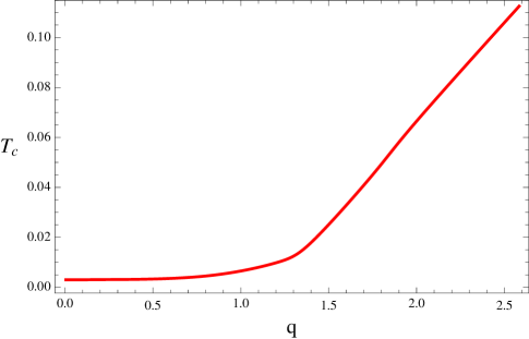
Figure 1: Critical temperature as a function of charge $q$ for the scaling case with $M^{2}=-2$ and $\hat{\tau}=1/\sqrt{3}$. The critical temperature at $q=0$ is $T_{c}\approx 0.00297$. There is no minimal charge, thus a neutral scalar will condense. We work in units in which the chemical potential is $\mu=1$.

In figure 2 we show the critical temperature as a function of $q$ for $M^{2}=-5/4$. In this case the index $\nu$ is real and the corresponding BF bound is unbroken. Just as expected, there is a minimal charge at which the background will become unstable to developing non-trivial scalar hair. We note that although the existence of a minimal charge is analogous to what would occur in AdS, the behavior of the charge term in the hyperscaling violating geometries is not – it is most important near $r_{tr}$ and negligible in the far IR.

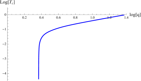
Figure 2: Critical temperature versus charge $q$ for the scaling case with $M^{2}=-5/4$ and $\hat{\tau}=1/\sqrt{3}$. We see a minimal charge $q\approx 2.327$ below which the zero mode for superfluid instability does not exist. We work in units in which the chemical potential is $\mu=1$.

VI.2 Non-scaling case with infinitely negative effective mass

Here we are considering the scenario discussed in case (i) of Section IV.2. The effective mass (43) approaches negative infinity as $r\rightarrow 0$. Thus, the expectation is that the zero mode should survive at arbitrarily small values of the charge. We consider the following coupling

$$B(\phi)=-2\cosh(\sqrt{3}\phi),$$ (98)

which is obtained from (88) by choosing $M^{2}=-2$ and $\hat{\tau}=\sqrt{3}$.

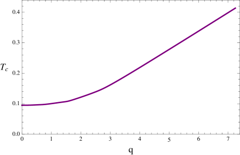
Figure 3: Critical temperature as a function of charge $q$ for the non-scaling case with $M^{2}=-2$ and $\hat{\tau}=\sqrt{3}$. The critical temperature at $q=0$ is $T_{c}\approx 0.0951$. We work in units with $\mu=1$.

Figure 3 shows the critical temperature as a function of charge $q$. One can clearly see that there is a phase transition even in the limit of zero charge. It is helpful to compare this case to the scaling one with $M^{2}=-2$, as they both share the same UV mass. Since the effective mass in the far IR goes to negative infinity, in the present case (with $\hat{\tau}=\sqrt{3}$) instabilities should be triggered much more easily than in the scaling one (with $\hat{\tau}=1/\sqrt{3}$). As a result, we expect the critical temperature here to be higher than that of the scaling scenario. This is precisely what we find from the numerics by comparing figure 3 with figure 1. Notice that this behavior is independent of how large $B_{0}\sim M^{2}$ is, a feature due entirely to the non-trivial coupling $B(\phi)$, which is absent in the standard holographic superconductor scenario. Thus, by appropriately choosing the functional dependence of the coupling, we can facilitate the phase transition and increase $T_{c}$.

VI.3 Remaining cases

In the remaining cases we discussed in Section IV.2, we don’t expect the zero mode to exist at arbitrarily small values of $q$. Let’s focus on the choice

$$B(\phi)=M^{2}\,,$$ (99)

which corresponds to $\hat{\tau}=0$ (or equivalently $\tau=0$) and falls under the category (iii) of Section IV.2. Before discussing the numerics, we stress that in these cases it’s hard to identify sharp analytical instability criteria in the scaling regime. The equation for the $\psi$ perturbation now reads

$$\psi^{\prime\prime}(\rho)-\frac{1}{\rho}\psi^{\prime}(\rho)-\frac{4(\sqrt{3}M^{2}\rho-q^{2})}{9\rho^{4}}\,\psi(\rho)=0,$$ (100)

and the solution in general is given by

$$\psi(\rho)=e^{\frac{2iq}{3\rho}}\left[c_{a}\,{}_{1}F_{1}\left(\frac{3}{2}-\frac{i\,M^{2}}{\sqrt{3}q},3,\frac{4iq}{3\rho}\right)+c_{b}\,U\left(\frac{3}{2}-\frac{i\,M^{2}}{\sqrt{3}q},3,\frac{4iq}{3\rho}\right)\right],$$ (101)

where ${}_{1}F_{1}(a,b,x)$ is the Kummer confluent hypergeometric function and $U(a,b,x)$ is a confluent hypergeometric function. The special case with $q=0$ needs to be treated separately, and is

$$\psi(\rho)=\rho\left[c_{a}\,I_{2}\left(\frac{4}{3^{3/4}}\sqrt{\frac{M^{2}}{\rho}}\right)+c_{b}\,K_{2}\left(\frac{4}{3^{3/4}}\sqrt{\frac{M^{2}}{\rho}}\right)\right]\,.$$ (102)

In contrast to the scaling case (97), it is not immediately apparent how to extract information about potential instabilities from the structure of the solutions. In particular, there is no simple analog of the generalized BF bound, illustrating the challenge of obtaining generic analytical conditions for the onset of the phase transition.

The behavior of the critical temperature as a function of charge $q$ for the choice $M^{2}=-2$ is presented in figure 4. Although we can not solve the system at very low temperatures, we find strong evidence that a minimal charge is indeed required in order to trigger the superfluid instability, as indicated by the effective mass and Schrodinger potential analysis.

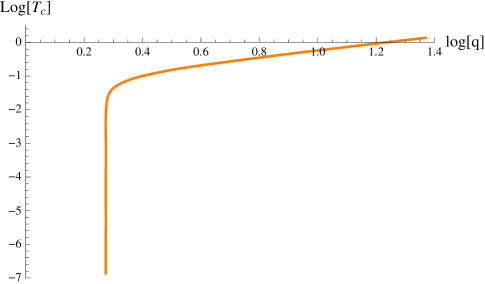
Figure 4: Log-Log plot of the critical temperature versus charge $q$ for the non-scaling case with $M^{2}=-2$ and $\hat{\tau}=0$. The critical temperature goes to zero at $q\approx 1.88$. We work in units with $\mu=1$.

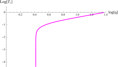
Figure 5: Log-Log plot of the critical temperature as a function of charge $q$ for the non-scaling case with $M^{2}=-5/4$ and $\hat{\tau}=0$. The critical temperature goes to zero at $q\approx 2.6$. We work in units with $\mu=1$.

A bigger value of $M^{2}=-5/4$ is then shown in figure 5. The qualitative behavior is very similar to that of figure 4. However, we note that as we increase the size of $M^{2}$, a bigger minimal charge is required in order to trigger the superfluid instability. This point can be understood qualitatively by comparing the Schrödinger potential (86) for different values of the mass (99) but keeping $q$ and $T$ fixed, as is done in figure 6. Recall that we are working in the grand canonical ensemble and have therefore fixed the chemical potential to $\mu=1$.

We choose parameters such that the thick magenta line in figure 6 corresponds to the zero mode solution of (87) for $M^{2}=-5/4,\hat{\tau}=0$ at $q\approx 2.6002$ and $T\approx 1.378\times 10^{-4}$. From (63), this case gives the smallest negative potential well which supports a zero mode bound state for the chosen values of $q$ and $T$ (e.g. for $k=1$ of (63)). One can in principle change $M^{2}$ to obtain a much larger negative potential region such that (63) can be satisfied for $k\geqslant 2$. However, it is easy to see from figure 6 that the range in which the Schrödinger potential is negative as well as its depth becomes smaller and smaller as one increases $M^{2}$. Therefore, in order to support a zero mode, a bigger value of $q$ is required to compensate for the increase in the mass parameter $M^{2}$. In addition, we note that there is a positive potential region in the deep IR, which is too small to see from figure 6.

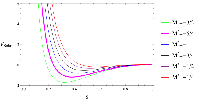
Figure 6: Schrödinger potential (86) as a function of radial coordinate $s=\frac{r_{h}+Q}{r+Q}$ for the non-scaling case $\hat{\tau}=0$. The different curves have the same values of charge $q\approx 2.6002$ and temperature $T\approx 1.378\times 10^{-4}$ but different values of $M^{2}$. The horizon is located at $s=1$ and the UV $AdS_{4}$ boundary at $s=0$. We choose parameters such that the thick magenta line corresponds to the zero mode solution for this particular choice of $q$ and $T$. We work in units of $\mu=1$.

Before closing this Section, we would like to point out one final feature visible from the numerics. As one can see from inspecting figures 1 to 5, when $q$ is large the value of $T_{c}$ increases linearly with $q$. This behavior can be understood as follows Cai:2013aca . Taking $q\rightarrow\infty$ while keeping $q\Psi$ and $qA_{\mu}$ finite, we arrive at the probe limit in which the gauge field and the charged scalar do not backreact on the background geometry. In order to compare our results with those in the probe limit, we have to perform the scaling transformation $\Psi\rightarrow q\Psi$ and $A_{\mu}\rightarrow qA_{\mu}$. After taking these rescalings into account, the physical dimensionless temperature becomes $T_{c}/q\mu$. Since we are working with $\mu=1$ (recall that we are in the grand canonical ensemble), this tells us that $T_{c}\propto q$, which is precisely what is observed from the numerics in the large charge limit. The backreacton of the $U(1)$ field and charged scalar on the geometry becomes smaller and smaller as $q$ is increased, explaining again why we observe a linear behavior for $T_{c}$ when the charge is large. We confirm this in figure 7, which has the same choice of parameters as figure 1, but reaches higher values of $q$. It is clear that the large $q$ behavior can be well approximated by the linear function $T_{c}=\gamma q$ with $\gamma$ a constant, as expected from the probe limit argument. For small charges we deviate from the linear relationship, as clearly visible from figure 1 as well as figure 7.

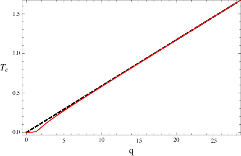
Figure 7: The red solid line is the critical temperature as a function of charge $q$ for the scaling case with $M^{2}=-2$ and $\hat{\tau}=1/\sqrt{3}$. The dashed black line corresponds to the probe limit result with $T_{c}/q\approx 0.586$. We work in units of $\mu=1$.

- (1) S. S. Gubser, “Breaking an Abelian gauge symmetry near a black hole horizon,” Phys. Rev. D 78, 065034 (2008) doi:10.1103/PhysRevD.78.065034 [arXiv:0801.2977 [hep-th]].
- (2) S. A. Hartnoll, C. P. Herzog and G. T. Horowitz, “Building a Holographic Superconductor,” Phys. Rev. Lett. 101, 031601 (2008) doi:10.1103/PhysRevLett.101.031601 [arXiv:0803.3295 [hep-th]].
- (3) S. A. Hartnoll, C. P. Herzog and G. T. Horowitz, “Holographic Superconductors,” JHEP 0812, 015 (2008) doi:10.1088/1126-6708/2008/12/015 [arXiv:0810.1563 [hep-th]].
- (4) S. A. Hartnoll, “Lectures on holographic methods for condensed matter physics,” Class. Quant. Grav. 26, 224002 (2009) doi:10.1088/0264-9381/26/22/224002 [arXiv:0903.3246 [hep-th]].
- (5) C. P. Herzog, “Lectures on Holographic Superfluidity and Superconductivity,” J. Phys. A 42, 343001 (2009) doi:10.1088/1751-8113/42/34/343001 [arXiv:0904.1975 [hep-th]].
- (6) G. T. Horowitz, “Introduction to Holographic Superconductors,” Lect. Notes Phys. 828, 313 (2011) [arXiv:1002.1722 [hep-th]].
- (7) R. G. Cai, L. Li, L. F. Li and R. Q. Yang, “Introduction to Holographic Superconductor Models,” Sci. China Phys. Mech. Astron. 58, no. 6, 060401 (2015) doi:10.1007/s11433-015-5676-5 [arXiv:1502.00437 [hep-th]].
- (8) S. K. Domokos and J. A. Harvey, “Baryon number-induced Chern-Simons couplings of vector and axial-vector mesons in holographic QCD,” Phys. Rev. Lett. 99, 141602 (2007) doi:10.1103/PhysRevLett.99.141602 [arXiv:0704.1604 [hep-ph]].
- (9) S. Nakamura, H. Ooguri and C. S. Park, “Gravity Dual of Spatially Modulated Phase,” Phys. Rev. D 81, 044018 (2010) doi:10.1103/PhysRevD.81.044018 [arXiv:0911.0679 [hep-th]].
- (10) H. Ooguri and C. S. Park, “Spatially Modulated Phase in Holographic Quark-Gluon Plasma,” Phys. Rev. Lett. 106, 061601 (2011) doi:10.1103/PhysRevLett.106.061601 [arXiv:1011.4144 [hep-th]].
- (11) A. Donos and J. P. Gauntlett, “Holographic striped phases,” JHEP 1108, 140 (2011) doi:10.1007/JHEP08(2011)140 [arXiv:1106.2004 [hep-th]].
- (12) O. Bergman, N. Jokela, G. Lifschytz and M. Lippert, “Striped instability of a holographic Fermi-like liquid,” JHEP 1110, 034 (2011) doi:10.1007/JHEP10(2011)034 [arXiv:1106.3883 [hep-th]].
- (13) S. A. Hartnoll and D. M. Hofman, “Locally Critical Resistivities from Umklapp Scattering,” Phys. Rev. Lett. 108, 241601 (2012) doi:10.1103/PhysRevLett.108.241601 [arXiv:1201.3917 [hep-th]].
- (14) G. T. Horowitz, J. E. Santos and D. Tong, “Optical Conductivity with Holographic Lattices,” JHEP 1207, 168 (2012) doi:10.1007/JHEP07(2012)168 [arXiv:1204.0519 [hep-th]].
- (15) A. Donos and S. A. Hartnoll, “Interaction-driven localization in holography,” Nature Phys. 9, 649 (2013) doi:10.1038/nphys2701 [arXiv:1212.2998].
- (16) D. Vegh, “Holography without translational symmetry,” arXiv:1301.0537 [hep-th].
- (17) M. Blake and D. Tong, “Universal Resistivity from Holographic Massive Gravity,” Phys. Rev. D 88, no. 10, 106004 (2013) doi:10.1103/PhysRevD.88.106004 [arXiv:1308.4970 [hep-th]].
- (18) A. Donos and J. P. Gauntlett, “Holographic Q-lattices,” JHEP 1404, 040 (2014) doi:10.1007/JHEP04(2014)040 [arXiv:1311.3292 [hep-th]].
- (19) T. Andrade and B. Withers, “A simple holographic model of momentum relaxation,” JHEP 1405, 101 (2014) doi:10.1007/JHEP05(2014)101 [arXiv:1311.5157 [hep-th]].
- (20) B. Goutraux, “Charge transport in holography with momentum dissipation,” JHEP 1404, 181 (2014) doi:10.1007/JHEP04(2014)181 [arXiv:1401.5436 [hep-th]].
- (21) A. Donos, B. Gout raux and E. Kiritsis, “Holographic Metals and Insulators with Helical Symmetry,” JHEP 1409, 038 (2014) doi:10.1007/JHEP09(2014)038 [arXiv:1406.6351 [hep-th]].
- (22) A. Salvio, “Transitions in Dilaton Holography with Global or Local Symmetries,” JHEP 1303, 136 (2013) doi:10.1007/JHEP03(2013)136 [arXiv:1302.4898 [hep-th]].
- (23) Z. Fan, “Holographic superconductors with hyperscaling violation,” JHEP 1309, 048 (2013) doi:10.1007/JHEP09(2013)048 [arXiv:1305.2000 [hep-th]].
- (24) A. Lucas and S. Sachdev, “Conductivity of weakly disordered strange metals: from conformal to hyperscaling-violating regimes,” Nucl. Phys. B 892, 239 (2015) doi:10.1016/j.nuclphysb.2015.01.017 [arXiv:1411.3331 [hep-th]].
- (25) E. Kiritsis and L. Li, “Holographic Competition of Phases and Superconductivity,” JHEP 1601, 147 (2016) doi:10.1007/JHEP01(2016)147 [arXiv:1510.00020 [cond-mat.str-el]].
- (26) H. Kodama and A. Ishibashi, “Master equations for perturbations of generalized static black holes with charge in higher dimensions,” Prog. Theor. Phys. 111, 29 (2004) doi:10.1143/PTP.111.29 [hep-th/0308128].
- (27) C. Keeler, G. Knodel and J. T. Liu, “What do non-relativistic CFTs tell us about Lifshitz spacetimes?,” JHEP 1401, 062 (2014) doi:10.1007/JHEP01(2014)062 [arXiv:1308.5689 [hep-th]].
- (28) N. Iqbal, H. Liu, M. Mezei and Q. Si, “Quantum phase transitions in holographic models of magnetism and superconductors,” Phys. Rev. D 82, 045002 (2010) doi:10.1103/PhysRevD.82.045002 [arXiv:1003.0010 [hep-th]].
- (29) M. Čubrović, “Confinement/deconfinement transition from symmetry breaking in gauge/gravity duality,” arXiv:1605.07849 [hep-th].
- (30) C. Charmousis, B. Goutraux, B. S. Kim, E. Kiritsis and R. Meyer, “Effective Holographic Theories for low-temperature condensed matter systems,” JHEP 1011, 151 (2010) doi:10.1007/JHEP11(2010)151 [arXiv:1005.4690 [hep-th]].
- (31) N. Iizuka, N. Kundu, P. Narayan and S. P. Trivedi, “Holographic Fermi and Non-Fermi Liquids with Transitions in Dilaton Gravity,” JHEP 1201, 094 (2012) doi:10.1007/JHEP01(2012)094 [arXiv:1105.1162 [hep-th]].
- (32) B. Gouteraux and E. Kiritsis, “Generalized Holographic Quantum Criticality at Finite Density,” JHEP 1112, 036 (2011) doi:10.1007/JHEP12(2011)036 [arXiv:1107.2116 [hep-th]].
- (33) L. Huijse, S. Sachdev and B. Swingle, “Hidden Fermi surfaces in compressible states of gauge-gravity duality,” Phys. Rev. B 85, 035121 (2012) doi:10.1103/PhysRevB.85.035121 [arXiv:1112.0573 [cond-mat.str-el]].
- (34) S. Harrison, S. Kachru and H. Wang, “Resolving Lifshitz Horizons,” JHEP 1402, 085 (2014) doi:10.1007/JHEP02(2014)085 [arXiv:1202.6635 [hep-th]].
- (35) J. Bhattacharya, S. Cremonini and A. Sinkovics, “On the IR completion of geometries with hyperscaling violation,” JHEP 1302, 147 (2013) doi:10.1007/JHEP02(2013)147 [arXiv:1208.1752 [hep-th]].
- (36) N. Kundu, P. Narayan, N. Sircar and S. P. Trivedi, “Entangled Dilaton Dyons,” JHEP 1303, 155 (2013) doi:10.1007/JHEP03(2013)155 [arXiv:1208.2008 [hep-th]].
- (37) S. Cremonini and A. Sinkovics, “Spatially Modulated Instabilities of Geometries with Hyperscaling Violation,” JHEP 1401, 099 (2014) doi:10.1007/JHEP01(2014)099 [arXiv:1212.4172 [hep-th], arXiv:1212.4172].
- (38) N. Iizuka and K. Maeda, “Stripe Instabilities of Geometries with Hyperscaling Violation,” Phys. Rev. D 87, no. 12, 126006 (2013) doi:10.1103/PhysRevD.87.126006 [arXiv:1301.5677 [hep-th]].
- (39) G. Knodel and J. T. Liu, “Higher derivative corrections to Lifshitz backgrounds,” JHEP 1310, 002 (2013) doi:10.1007/JHEP10(2013)002 [arXiv:1305.3279 [hep-th]].
- (40) S. Cremonini, “Spatially Modulated Instabilities for Scaling Solutions at Finite Charge Density,” arXiv:1310.3279 [hep-th].
- (41) S. Barisch-Dick, G. L. Cardoso, M. Haack and . V liz-Osorio, “Quantum corrections to extremal black brane solutions,” JHEP 1402, 105 (2014) doi:10.1007/JHEP02(2014)105 [arXiv:1311.3136 [hep-th]].
- (42) D. K. O’Keeffe and A. W. Peet, “Electric hyperscaling violating solutions in Einstein-Maxwell-dilaton gravity with corrections,” Phys. Rev. D 90, no. 2, 026004 (2014) doi:10.1103/PhysRevD.90.026004 [arXiv:1312.2261 [hep-th]].
- (43) J. Bhattacharya, S. Cremonini and B. Gout raux, “Intermediate scalings in holographic RG flows and conductivities,” JHEP 1502, 035 (2015) doi:10.1007/JHEP02(2015)035 [arXiv:1409.4797 [hep-th]].
- (44) S. S. Gubser, “Curvature singularities: The Good, the bad, and the naked,” Adv. Theor. Math. Phys. 4, 679 (2000) [hep-th/0002160].
- (45) A. Lucas, S. Sachdev and K. Schalm, “Scale-invariant hyperscaling-violating holographic theories and the resistivity of strange metals with random-field disorder,” Phys. Rev. D 89, no. 6, 066018 (2014) doi:10.1103/PhysRevD.89.066018 [arXiv:1401.7993 [hep-th]].
- (46) J. Gath, J. Hartong, R. Monteiro and N. A. Obers, “Holographic Models for Theories with Hyperscaling Violation,” JHEP 1304, 159 (2013) doi:10.1007/JHEP04(2013)159 [arXiv:1212.3263 [hep-th]].
- (47) G. T. Horowitz and M. M. Roberts, “Zero Temperature Limit of Holographic Superconductors,” JHEP 0911, 015 (2009) doi:10.1088/1126-6708/2009/11/015 [arXiv:0908.3677 [hep-th]].
- (48) S. S. Gubser and F. D. Rocha, “Peculiar properties of a charged dilatonic black hole in ,” Phys. Rev. D 81, 046001 (2010) doi:10.1103/PhysRevD.81.046001 [arXiv:0911.2898 [hep-th]].
- (49) S. A. Hartnoll and E. Shaghoulian, “Spectral weight in holographic scaling geometries,” JHEP 1207, 078 (2012) doi:10.1007/JHEP07(2012)078 [arXiv:1203.4236 [hep-th]].
- (50) A. Donos and S. A. Hartnoll, “Universal linear in temperature resistivity from black hole superradiance,” Phys. Rev. D 86, 124046 (2012) doi:10.1103/PhysRevD.86.124046 [arXiv:1208.4102 [hep-th]].
- (51) R. J. Anantua, S. A. Hartnoll, V. L. Martin and D. M. Ramirez, “The Pauli exclusion principle at strong coupling: Holographic matter and momentum space,” JHEP 1303, 104 (2013) doi:10.1007/JHEP03(2013)104 [arXiv:1210.1590 [hep-th]].
- (52) A. Donos, J. P. Gauntlett and C. Pantelidou, “Semi-local quantum criticality in string/M-theory,” JHEP 1303, 103 (2013) doi:10.1007/JHEP03(2013)103 [arXiv:1212.1462 [hep-th]].
- (53) R. G. Cai, L. Li and L. F. Li, “A Holographic P-wave Superconductor Model,” JHEP 1401, 032 (2014) doi:10.1007/JHEP01(2014)032 [arXiv:1309.4877 [hep-th]].