MultiDK: A Multiple Descriptor Multiple Kernel Approach for Molecular Discovery and Its Application to The Discovery of Organic Flow Battery Electrolytes

Abstract

We propose a multiple descriptor multiple kernel (MultiDK) method for efficient molecular discovery using machine learning. We show that the MultiDK method improves both the speed and the accuracy of molecular property prediction. We apply the method to the discovery of electrolyte molecules for aqueous redox flow batteries. Using multiple-type - as opposed to single-type - descriptors, more relevant features for machine learning can be obtained. Following the principle of the ’wisdom of the crowds’, the combination of multiple-type descriptors significantly boosts prediction performance. Moreover, MultiDK can exploit irregularities between molecular structure and property relations better than the linear regression method by employing multiple kernels - more than one kernel functions for a set of the input descriptors. The multiple kernels consist of the Tanimoto similarity function and a linear kernel for a set of binary descriptors and a set of non-binary descriptors, respectively. Using MultiDK, we achieve average performance of $r^{2}=0.92$ with a set of molecules for solubility prediction. We also extend MultiDK to predict pH-dependent solubility and apply it to solubility estimation of quinone molecules with ionizable functional groups as strong candidates of flow battery electrolytes.

1 Introduction

Aqueous organic flow batteries are emerging as a low-cost alternative to store renewable energy ^{1, 2, 3, 4, 5}. For example, Huskinson et al., Yang et al., and Liu et al. experimentally showed that high capacity energy storage can be achieved using earth abundant organic electrolytes such as quinone molecules ^{6, 7}. Given the vast molecular space covered by all possible quinone molecules, high-throughput computational screening ^{8, 9, 10, 11, 12, 13, 14, 15, 16, 17, 18, 19, 20} is important to find electrolytes that satisfy the stringent requirement of aqueous flow batteries. In particular, the flow battery system in ¹ requires a redox potential greater than 0.9V for a catholyte and less than 0.2V for an anolyte, as well as a solubility greater than one molar for both electrolytes. Moreover, quinone electrolytes operating in acid (pH 0) and alkaline (pH 14) flow battery environments were demonstrated in ¹ and ³, respectively.

Recent high-throughput computational screening of benzo-, naphtho-, anthra-, and thiopheno-quinone libraries ^{21, 22} demonstrated that the reduction potential of these redox couples can be predicted accurately utilizing molecular quantum chemistry methods and linear regressions. Using the free energy of solvation as a proxy descriptor, the molecular solubility of electrolytes was also predicted in both references. Here, we build upon this work by developing a machine learning strategy that results in strong correlations with experimental solubility data predicts the required molecular properties in order to accelerate molecular screening by several orders of magnitude.

The computational prediction of molecular solubility has been a research topic for decades, with most research being driven by the field of drug discovery ^{23, 24, 6}. However, predicting the solubility of organic electrolytes is particularly challenging, given the stringent target solubilities and the extreme pH values of flow battery electrolyte solutions ²⁵. While the target solubility of drug molecules is generally less than 0.1 molar, the target for flow battery organic electrolytes can be more than 1 molar. Moreover, molecular libraries to screen potential flow battery electrolytes include extremely acidic ²⁵ or basic organic molecules ³ while the majority of drug candidates are relatively weak acids and bases ^{23, 26, 18, 27}.

Both machine learning and quantum chemical approaches can be used to estimate molecular solubility. Whereas machine learning approaches predict solubility based on training to experimental data ^{28, 29, 30}, quantum chemistry aims to predict solubility from first principles ^{21, 31, 32, 33}. Although quantum chemical approaches are preferable for obtaining a mechanistic understanding of underlying principles ^{31, 24}, our focus here is on machine learning approaches which facilitate high-throughput and artificially-intelligent molecular discovery ^{28, 34, 35}.

Machine learning approaches can be categorized into three types of methods according to the types of descriptors used: property-based methods, structure-based methods, and functional group-based methods (Table 1). Property-based methods predict physicochemical values based on molecular properties which can be measured experimentally or obtained from computational approaches. One such property used for solubility estimation is the partition coefficient, the logarithm of which is denoted as logP ^{36, 37, 38, 39}. Several methods have been proposed to calculate logP ^{40, 41, 42, 43}. The general solubility estimation method (GSE), with its extended and modified variants, is an example of a property-type method which estimates logS from logP ^{36, 37, 38, 39, 44}. On the other hand, structure-based methods rely on the estimation of solubility as a function of molecular structure. Structure is usually represented by a binary fingerprint, consisting of molecular topology, connectivity, or fragment information ^{45, 46}. Finally, group-based methods partition molecules into functional groups, and the contribution of each to the value of a physicochemical property is estimated ^{47, 48, 49}.

Property-based methods generally involve fewer regression parameters than the other two approaches, but require additional computation in order to estimate intermediate properties included in the descriptor set. If large experimental data is available for intermediate properties such as logP, property-based methods can predict solubility for a wider range of molecules than any of the other methods ^{50, 51}. However, a significant gap between logP-based estimation and experimental solubility still remains ³⁸. Large efforts have been devoted to reduce this gap by adding more input information to the set of descriptors, with a concomitant increase in the complexity of the regressions employed ²³.

Two examples of property-based methods, the GSE approach and Delaney’s extended GSE (EGSE) approach, rely on two and three fitted parameters, respectively. In ³⁸, the prediction performances of GSE and EGSE were shown to be $r^{2}(\mathrm{GSE})=0.67$ and $r^{2}(\mathrm{EGSE})=0.69$ for a dataset of 1305 compounds compiled by the authors, which highlights the gap between prediction and experiment for such methodologies.

Structure-based methods predict solubility directly from molecular structural information, which can be implemented by various types of descriptors ^{52, 53, 46, 54}. Generally, binary fingerprints offer a good trade-off between simplicity and predictive power ^{45, 55, 49}. We recently developed the concept of neural fingerprints which are structure-based and application-specific with input descriptors generated for arbitrary size and shape based on a molecular graph ⁵⁴.

Zhou et al. predicted molecular solubility using a binary circular fingerprint descriptor ⁴⁵. Although they demonstrated a prediction performance of $r^{2}=0.83$, the authors had to carefully select the training data set in order to achieve that value of $r^{2}$. Huuskonen showed that a prediction performance of $r^{2}=0.92$ can be achieved by using non-binary descriptors consisting of 53 parameters, including 39 atom-type electro-topological state (E-state) indices ²⁵. However, non-binary descriptors significantly increase computational cost in both the training and validation stages, especially when feature selection is encountered during the regression process ^{56, 57}. A different binary fingerprint approach has been investigated by Lind and Maltseva, in which support vector regression employing the Tanimotto similarity kernel is applied in order to overcome the limit of the multiple linear regression method ⁵⁵.

The group-based methods integrate contributions of all associated functional groups multiplied by the number of each functional group in a compound: $C_{0}+\sum_{i=1}^{N}C_{i}G_{i}$ where $G_{i}$ is the number of times the $i$th group appears in the compound, $C_{0}$ is a constant bias parameter, and $C_{i}$ is the contribution of the $i$th group ⁴⁷. Hou et al. proposed an atom contribution method, which overcomes the ’missing fragment’ problem in pure group contribution methods ⁵⁸. The atom contribution method categorizes atoms together with their surrounding molecular environment. Cheng et al. used functional key descriptors such as MACCS Keys and PC881 instead of directing counting numbers of each functional group. This approach simplifies descriptor values to be binary form but ’missing fragment’ and requiring a large training data set are still unavoidable for the cases of small and large number of the keys, respectively. Moreover, Cheng et al. apply them for solubility classification task with a much lower solubility requirement, 10 $\mu$g/mL, than the threshold values necessory for aqueous flow battery applications.

Category	Methods
Machine Learning	Property-based method 36, 37, 38, 39
	Structure-based method 25, 55, 45
	Group-based method 47, 48, 49
Quantum Calculation 25, 31, 24, 21

Table 1: A categorization of solubility estimation methods. First, machine learning and quantum calculation methods are depicted. The machine learning methods include the property-based, structure-based and group-based method.

The ability to carry out solubility predictions that account for pH-dependence is critical to discovering molecules for aqueous flow batteries. In addition to mandating very high solubility, the pH required to operate an organic flow battery system varies depending on the required redox potential values and other experimental considerations. For instance, negative electrolytes of 9,10-anthraquinone-2,7-disulphonic acid (AQDS) in ¹ and 2,6-dihydroxyanthraquinone (DHAQ) ³ require 1 molar solubility at pH 0 and pH 14, respectively. While prediction methods for intrinsic solubility have been widely discussed, methods to predict pH-dependent solubility have remained less explored ^{59, 27, 60, 26, 24, 61}. In theory, the Henderson-Hasselbach relationship can be used to predict pH-dependent solubility based on the intrinsic solubility of a molecule ⁶⁰. However, the limitations of current pKa prediction accuracies as well as the salt plateau phenomena of ionic solubility encourage the use of a data-driven approaches. This requires significantly more experimental training data (solubility as a function of pH) than intrinsic solubility prediction ^{27, 61}. Moreover, the intrinsic solubility of extremely strong acids with a negative pKa value has not been well investigated in the literature.

In high-throughput molecular screening, the development of an accurate and cost-effective property estimation method is a key factor for successfully finding new candidate molecules ^{62, 54, 63}. In this work, we develop a fast and accurate property estimation method for high-throughput molecular discovery. We named the proposed approach a multiple descriptor multiple kernel (MultiDK) method. The method relies on combining an ensemble of different descriptors, including fingerprints, functional keys, as well as other molecular physicochemical properties. We also apply different kernels for different types of descriptors to overcome intrinsic irregularities between a fingerprint and a property ⁵⁵. Both intrinsic and pH-dependent solubility estimations are supported by the MultiDK approach.

2 Methods

2.1 Datasets and Tools

We tested the performance of MultiDK on four datasets. The four datasets include 1676 molecules from ⁶⁴, 496 molecules from ⁶⁵, 1140 molecules from ³⁸ and 3310 molecules from ³⁹. The 1676 molecule dataset includes most of the 1297 molecules in ²⁵. The tests were performed using 20-fold cross-validation. In this work, we use Python packages including Pandas ⁶⁶, Scikit-learn ⁶⁷, Tensorflow ⁶⁸ and Seaborn ⁶⁹ for data manipulation, machine-learning, and visualization tools.

2.2 MultiDK method

In this paper, we compare the prediction performance of the MultiDK method against single descriptor (SD) and multiple descriptor (MD) methods. The SD method uses only one type of a descriptor, such as a Morgan fingerprint, MACCS keys or a specific molecular physicochemical property. Morgan fingerprints represent an atom and path structure of a molecule using a binary hashing procedure. MACCS keys represent functional group information. For molecular properties, we include molecular weight, Labute’s approximate surface area (LASA), or the logarithm partition coefficient (logP). The MD and MultiDK methods include more than one descriptor. Both the Morgan fingerprint and the MACCS keys are binary descriptors while the physicochemical molecular property is a non-binary, real-valued descriptor.

The MultiDK approach predicts the target molecular property as follows:

$$y=\sum_{i=1,\ldots,L}w^{\mathrm{B}}_{i}k_{B}(\mathbf{x}^{\mathrm{B}},\mathbf{x}^{\mathrm{B}}_{i})+\mathbf{w}^{\mathrm{NB}}\mathbf{x}^{\mathrm{NB}}+w_{0}$$ (1)

where $\mathbf{x}^{B}$ and $\mathbf{x}^{NB}$ are binary and non-binary descriptor vectors, respectively. $\mathbf{x}^{B}_{i}$ is a binary descriptor vector for the $i$th training molecule, $\mathbf{w}^{B}$ and $\mathbf{w}^{NB}$ are weight vectors corresponding to $\mathbf{x}^{B}$ and $\mathbf{x}^{NB}$ , respectively, $L$ is the number of a training molecules, and $k_{B}(\cdot)$ is a binary kernel function.

Rather than using a single kernel or linear regression, MultiDK utilizes multiple kernels such as a nonlinear binary kernel for binary descriptors and linear processing for non-binary descriptors separately. To optimize a kernel function ^{70, 71, 72}, multiple combinatorial kernels have been used in various applications including biomedical data ⁷³ and YouTube video data ^{74, 75}. Here, we use a multiple kernel approach to apply appropriate kernels for different features instead of training the kernel. The binary kernel function of $k_{B}(\cdot)$ contributes by exploiting a non-linear relationship between the molecular structure and property. The non-linear relationships arise primarily because each bit indicates the presence or absence of a pattern rather than a quantitative value. MultiDK uses all training molecules as support vector molecules for kernel processing similar to support vector machines. We use the Tanimoto kernel which has been used in a wide range of machine learning applications, such as exploiting binary feature information to recognize white images on a black background ⁷⁶ as well as a kernel for support vector and Gaussian progress regression in molecular property prediction ^{55, 8}.

In the MultiDK approach, ensemble learning is employed based on multiple combinational descriptors according to the principle of the ’wisdom of the crowds’ ⁷⁷. The set of descriptors in MultiDK includes the Morgan circular fingerprints ⁵³, MACCS Keys ⁴⁶ fingerprints and three non-binary molecular properties. The three types of descriptors represent structure hash (atom, path) and structure pattern (key, functional group) and target related molecular properties. We find that this ensemble combination is effective to predict molecular properties because both atom and subgroup representations are employed in the set of descriptors together with the related molecular properties. Moreover, we use different kernels for binary and non-binary descriptors. Particularly, a binary similarity kernel is applied to the binary descriptor and a linear kernel for the non-binary descriptor.

We evaluate the methods with training and cross-validation phases. In the training phase, we optimize the regression parameters using Ridge regularization. The descriptor consists of 4096 binary bits of the Morgan circular fingerprint with radius 6, 117 binary bits of the MACCS Keys and a few non-binary scalar descriptors. We generate all descriptors using the RDKit tool ⁷⁸ except for the partition coefficient, which we obtain from Cxcalc from the Chemaxon Marvin suite ⁷⁹. Before linear regression, we pre-process the 4213 binary bits with the binary similarity kernel by calculating the Tanimoto similarity between an input vector and the set of training vectors. We pass the non-binary descriptors directly to the linear regression stage without pre-processing. Then, the binary kernel output values and the direct non-binary output value are entered into the Ridge linear regression stage. We employ the Ridge regression routine in the scikit-learn Python package ⁸⁰. The regularization process eventually produces the best regression coefficients and an intercept corresponding to the maximum $R^{2}$ performance. In the cross-validation phase, a combination vector of the binary kernel outputs and a direct descriptor of a test molecule is multiplied by the coefficients obtained in the training phase.

2.3 MultiDK for estimating intrinsic solubility, logS

We use MultiDK for solubility prediction as follows:

$$\log S=\sum_{i=1,\ldots,L}w^{\mathrm{CK}}_{i}k_{B}(\mathbf{x}^{\mathrm{CK}},\mathbf{x}^{\mathrm{CK}}_{i})+(\mathbf{w}^{\mathrm{WSP}}\cdot\mathbf{x}^{\mathrm{WSP}})+w_{0}$$ (2)

where the subindices C, K, W, S, and P represent the Morgan circular fingerprint, the MACCS keys, the molecular weight, Labute’s approximate surface area (LASA) (Labute 2000) and the logarithm partition coefficient (logP), respectively. $L$ is the number of a training molecules, $k_{B}(\cdot)$ is a binary kernel function, $\mathbf{x}^{MCMK}=[\mathbf{x}^{MC},\mathbf{x}^{MK}]$ is a concatenated binary vector for an input molecule, $\mathbf{x}^{a}_{i}$ is a concatenated binary vector of the $i$th supporting molecule, and $x^{\mathrm{MW}}$ is molecular weight (MW). Both $w^{\mathrm{MCMK}}_{i}$ and $w^{\mathrm{MW}}$ are regression coefficients and $w_{0}$ is the regression intercept. The values of $\mathbf{x}^{\mathrm{MC}}$, $\mathbf{x}^{\mathrm{MK}}$ and $x^{\mathrm{MW}}$ are generated according to the SMILES string of a molecule.

2.4 MultiDK for estimating pH dependent solubility, logS(pH)

In order to predict pH-dependent solubility, we extend the MultiDK method as follows:

$$\log S(\mathrm{pH})=\log S+\log P-\log D(\mathrm{pH})$$ (3)

where $\log P$ and $\log D(\mathrm{pH})$ are the $n$-octanol-to-water partition coefficient and the pH-dependent distribution coefficient, respectively. Since the two coefficients can be approximated as $\log P=\log S_{\mathrm{Oct}}-\log S$ and $\log D(\mathrm{pH})=\log S_{\mathrm{Oct}}-\log S(\mathrm{pH})$ ^{36, 37}, we are able to extend MultiDK as in (3) where $\log S_{\mathrm{Oct}}$ is solubility in octanol. The octanol solubility is intrinsic and therefore determined regardless of existence of ionizable groups ⁸¹. We evaluate both $\log P$ and $\log D(\mathrm{pH})$ using the cxcalc plugin in the Chemaxon Marvin suite ⁸².

3 Results and Discussion

3.1 Cross-validation results

3.1.1 Performance of MultiDK for solubility prediction

We use $r^{2}$ distribution of 20-fold cross validation as a metric of prediction performance. The $r^{2}$ distribution is obtained by 20 time repetition of both training and testing until 20 subsets of data are all used for validation. Figure 1 shows the $r^{2}$ distribution obtained with each of the methods tested as a function of the Ridge regression hyper-parameter $\alpha$. Here, we used the 1676 unique molecules in ⁶⁴. For efficient comparison, only one non-binary descriptor is considered in this evaluation. Both the MultiDK and the MD methods employ two binary and one non-binary descriptors where the two binary and one non-binary descriptors are Morgan fingerprints (MFP), MACCS Keys (MACCS) and molecular weight (MolW). As shown in the figures, MultiDK and MD significantly outperform SD. Moreover, MultiDK is most robust to changes in the value of $\alpha$. This result reveals that additional group and property information help improve the regression performance.

In Figure 2, the performances of SD family, MD and MDMK are compared when the optimal value of $\alpha$ is used, where the SD family includes MFP, MACCS and MolW. This bar graph shows a clear difference between the SD family, MD and MultiDK approaches. The best $\alpha$ value are found by a grid search approach which selects $\alpha$ on the basis of regression performance in the range of $10^{-3}$ to $10^{2}$ with 10 logarithmically equally spaced steps. Each regression performance is evaluated using a 20-fold cross-validation with initial data shuffling. SD (MFP), MD and MDMK achieve their best regression coefficient values of $r^{2}$ $\pm$ std($r^{2}$) = 0.72 $\pm$ 0.04, 0.86 $\pm$ 0.04 and 0.89 $\pm$ 0.03 at $\alpha=$ 10.0, 31.6 and 0.03, respectively. This result highlights three important points. First, SD with MFD outperforms the other two SDs approaches, SD using MACCS and SD using MolW. It suggests that detailed structural information helps to estimate solubility. MolW is one non-binary value and MACCS and MFB consist of 117 and 4069 binary values, respectively. Second, both MD and MultiMK outperform SD, which emphasizes the necessity of multiple type descriptors for accurately estimating molecular properties. Third, MultiDK can further improve prediction performance in comparison to MD through the use of a binary kernel regression.

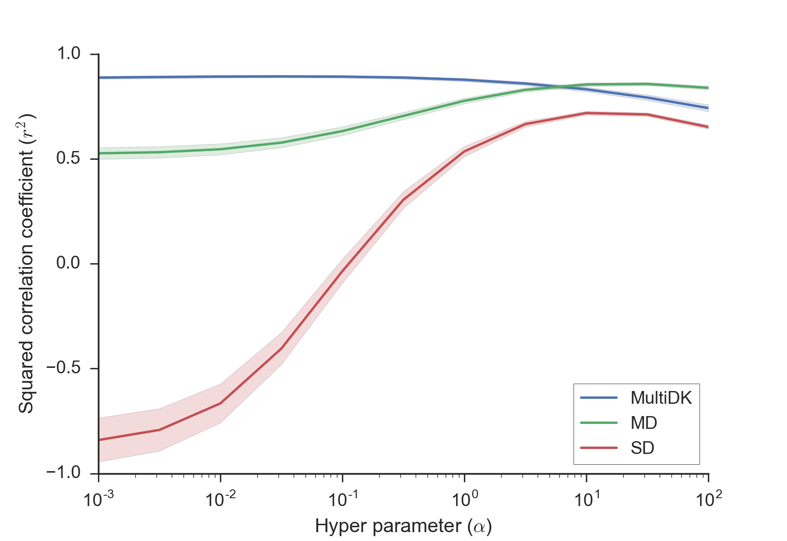
Figure 1: Solubility prediction as a function of the Ridge regression hyperparameter $\alpha$ for the SD, MD and MDMK cases. For each $\alpha$ in $10^{-3}$ to $10^{2}$, a 20-fold cross-validation was applied.

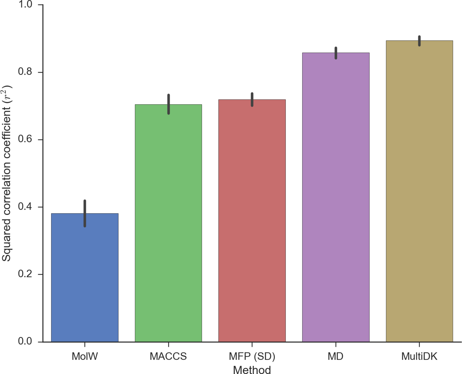
Figure 2: , the performances of SD, MD and MDMK are compared when the optimal value of $\alpha$ is used. For SD, molecular weights (MolW), MACCS Keys (MACCS) and Morgan fingerprint (MFP or SD) are independently used as a descriptor.

3.1.2 Performance of MultiDK with more descriptors

The $r^{2}$ distributions of different methods on the 1676 molecules using more descriptors are shown in Figure 3 where the box represents the interquartile range of $r^{2}$ values, i.e., the difference between the first quartile and the second quartile, and the median of them is drawn inside the box. The numerical values of them are shown in Table 2. We include two more non-binary descriptors which are Labute’s approximate surface area (LASA) ⁸³ and the logarithm partition coefficient (logP). Paricularly for MultiDK, we include a method with separate binary kernels for each binary descriptor. MD$xy$ and MultiDK$xy$ represent a method which embeds $x$ binary and $y$ non-binary descriptors. Figure 4 shows a comparison of the experimental data and the MultiDK results obtained through cross-validation with the best $\alpha$. We obtained the following cross-validation summary statistics: mean($r^{2}$) = 0.91, std($r^{2}$) = 0.027, root mean squared error (RMSE) = 0.61, mean absolute error (MSE) = 0.45, median absolute error (MSE) = 0.33.

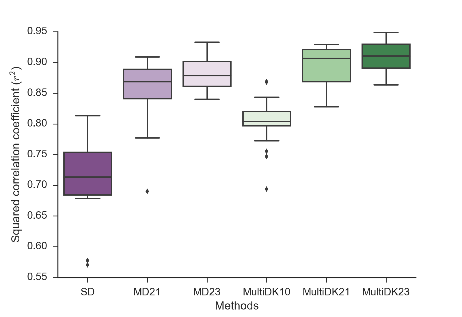
Figure 3: Prediction performance of different methods with the dataset with 1676 molecules.

Method	Best $\alpha$	E[$r^{2}$]	std($r^{2}$)
SD	1E+1	0.72	0.06
MD21	3E+1	0.86	0.05
MD23	3E+1	0.88	0.03
MultiDK10	1E-3	0.80	0.04
MultiDK21	3E-2	0.89	0.04
MultiDK23	1E-1	0.91	0.03

Table 2: 20-fold cross-validation performances of the 1676 molecules

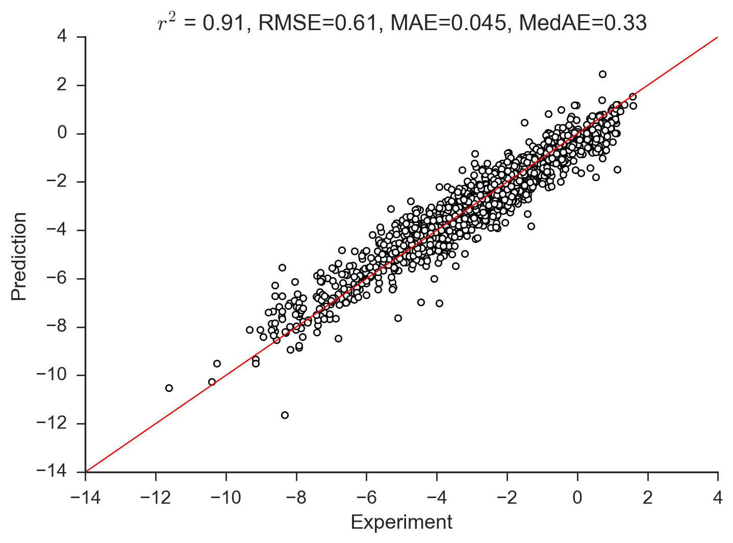
Figure 4: Comparision of the 1676 experimental solubility data and cross-validation results of MultiDK using the optimal value of $\alpha$.

3.1.3 Performance of MultiDK for other datasets

The three more datasets of 496 molecules ⁶⁵, 1140 molecules ³⁸ and 3310 molecules ³⁹ are considered in order to verify the proposed MultiDK method as shown in Figures 5, 6, and 7, respectively. The average values and standard deviation of $r^{2}$ obtained across multiple cross validation iterations are illustrated in Table 3. From the figures and the table, we confirm that the performance of MultiDK are better than MD for all new three data sets when the same input descriptors are used. Moreover, SD with only MFP is shown to be the worst among all cases, which is equivalent to the previous 1676 molecule case.

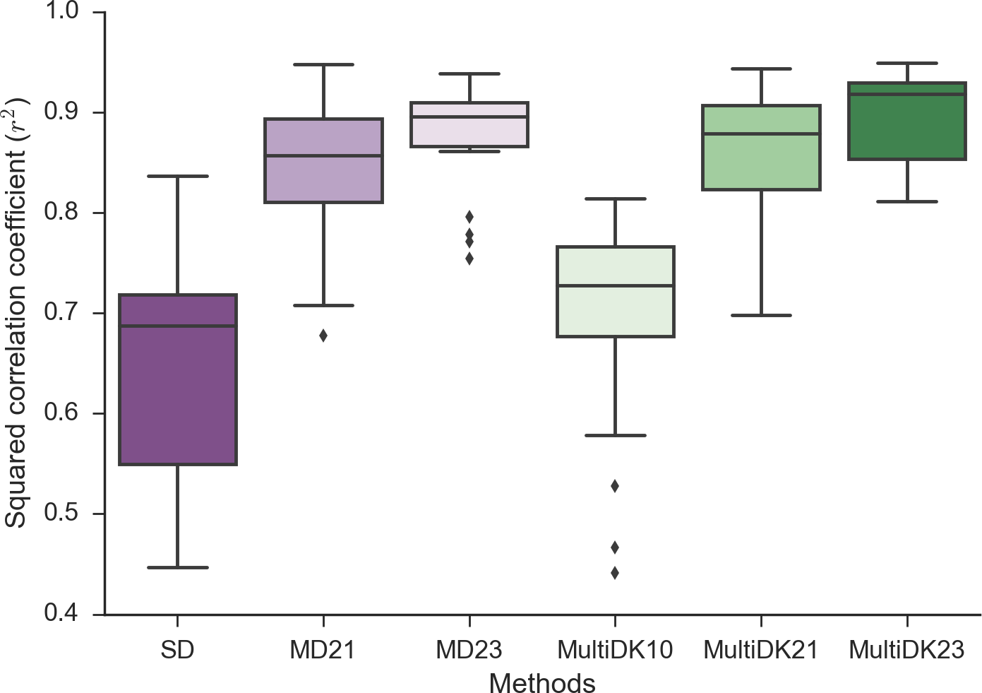
Figure 5: Prediction performance of different methods with the dataset with 496 molecules.

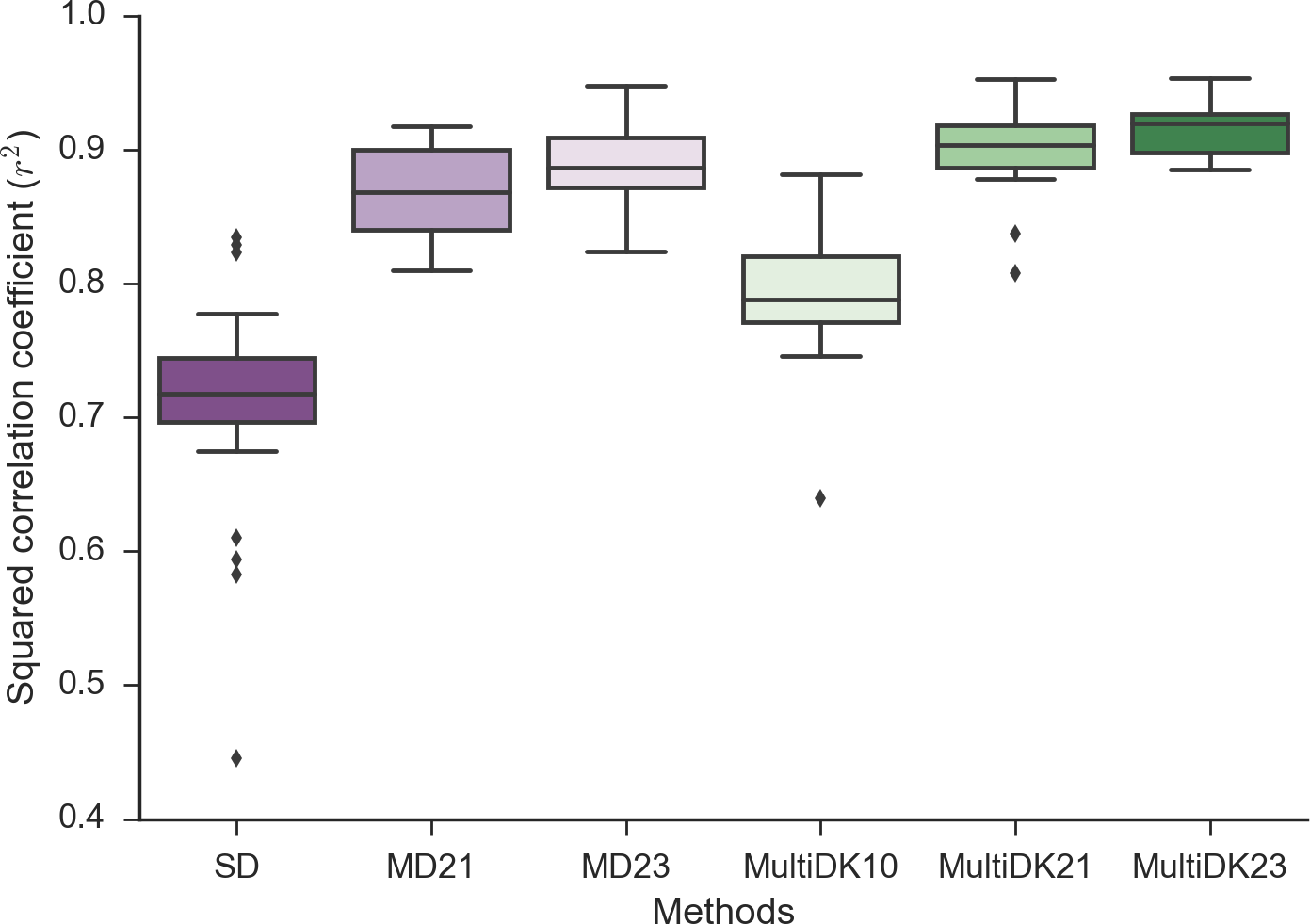
Figure 6: Prediction performance of different methods with the dataset with 1140 molecules.

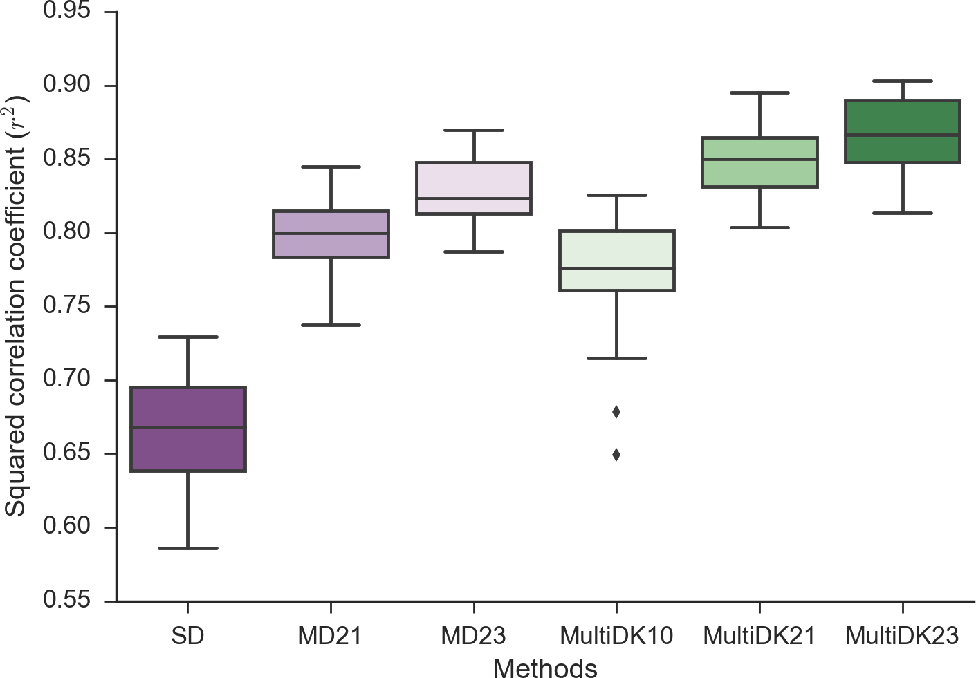
Figure 7: Prediction performance of different methods with the dataset with 3310 molecules.

Method	496 molecules			1140 molecules			3310 molecules
	Best $\alpha$	E[$r^{2}$]	std($r^{2}$)	Best $\alpha$	E[$r^{2}$]	std($r^{2}$)	Best $\alpha$	E[$r^{2}$]	std($r^{2}$)
SD	1E+1	0.65	0.12	1E+1	0.71	0.09	3E+1	0.66	0.05
MD21	1E+1	0.84	0.07	1E+1	0.87	0.04	3E+1	0.79	0.06
MD23	1E+1	0.88	0.06	1E+1	0.89	0.03	3E+1	0.83	0.02
MultiDK10	3E-3	0.70	0.11	3E-3	0.79	0.05	3E-2	0.77	0.05
MultiDK21	7E-2	0.86	0.06	3E-2	0.90	0.04	1E-1	0.85	0.03
MultiDK23	7E-2	0.89	0.05	3E-2	0.92	0.02	1E-1	0.87	0.04

Table 3: Performances of solubility prediction for different datasets

3.2 Application to the prediction of quinone electrolytes

3.2.1 Intrinsic solubility prediction of quinone molecules

Next, we apply the MultiMK method to predict the solubility of a set of quinone molecules, which are useful electrolytes for organic aqueous flow batteries. The intrinsic solubility is defined as the solubility of a molecule in its neutral form. Three types of quinone families, benzoquinones (BQ), naphthoquinones (NQ) and anthraquinones (AQ) as shown in Figure 8, were considered.

We tested molecules belonging to the BQ, NQ and AQ with no or one substituent R-group, where the number of the total test molecules are 27 consisting 5 BQ, 13 NQ and 9 AQ family molecules. The intrinsic solubility was predicted using three different methods: MultiDK, VCCLAB and EGSE. VCCLAB is an on-line solubility estimation tool (http://www.vcclab.org/lab/alogps/) and EGSE estimates the intrinsic solubility as:

$$\log S=0.16-0.63C\log P-0.0062\mathrm{MW}+0.066\mathrm{RB}-0.74\mathrm{AP}$$ (4)

where MP is the melting point, MW is the molecular weight, RB is a rotational bond ,and AP is an aromatic portion of the molecule. VCCLAB estimates solubility by training 1291 molecules using an artificial neural network ⁸⁴. As shown in Figure 9, regardless of the molecule types or the attached R-groups, all three methods predict the intrinsic solubility (logS) of the molecules to be below zero log-molar. Thus, all molecules have intrinsic solubility less than the solubility target of the aqueous flow battery.

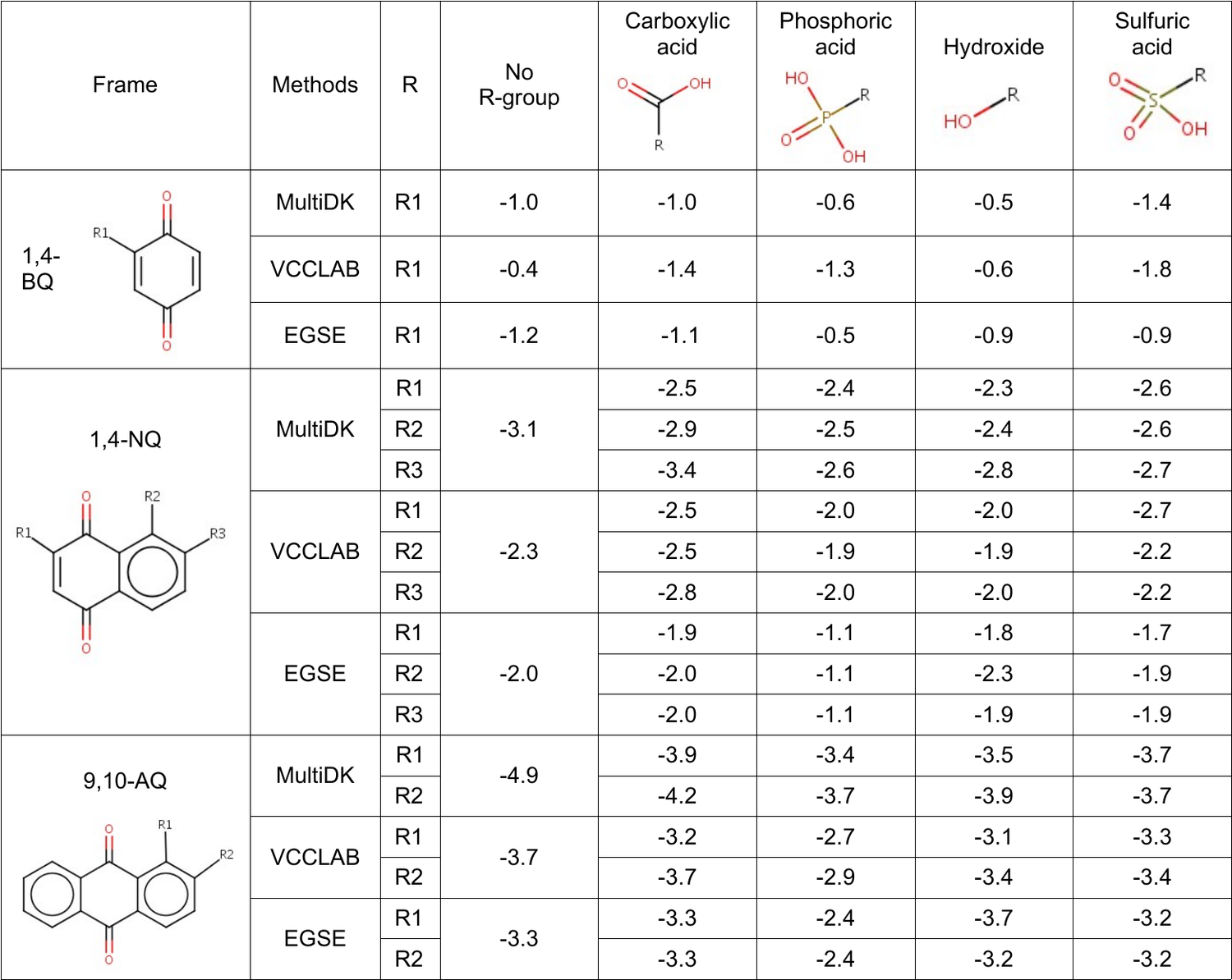
Figure 8: Predicted solubility of 27 quinone molecules by three different methods, i.e., MultiDK, VCCLAB and EGSE, where Benzoquinone (BQ), naphthoquinone (NQ) and anthraquinone (AQ), with available unique positions of R-group attachment.

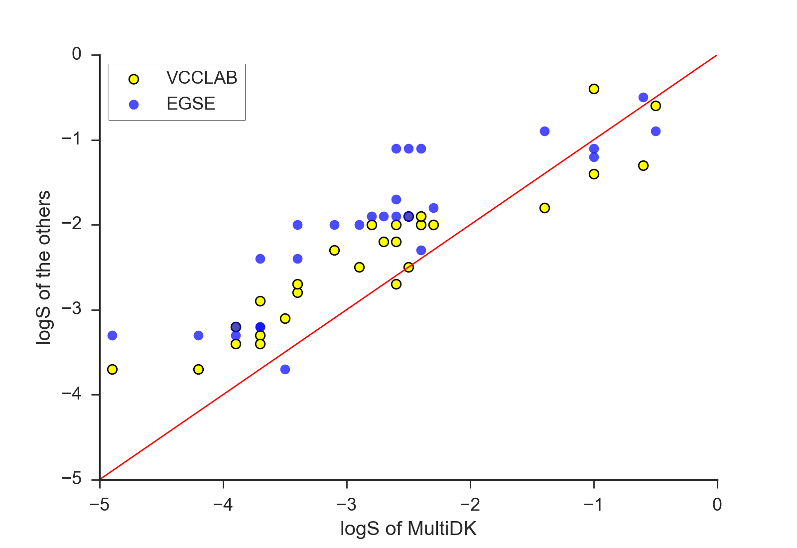
Figure 9: Three sets of predicted solubility values for 27 quinones compared against each other. Solubility values were predicted using the MultiDK, VCCLAB and EGSE methods. The three methods show that the predicted intrinsic solubility values of the 27 quinones are lower than 0 log molar, regardless of the attached functional group. 0 log molar is the general solubility requirement of electrolytes for inexpensive organic aqueous flow battery applications.

3.2.2 pH-dependent solubility for single R-group quinones

In Figure 10, 11 and 12, we show pH-dependent solubility predicted by the extended MultiDK method. We applied the extended method to the three types of quinone family molecules. Figure 10 shows the predicted pH-dependent solubility for five BQ molecules which are BQ with a sulfonic acid (SO₃H), phosphori acid (PO₃H), carboxylic acid (COOH) and hydroxide (OH) or no R group. The BQ with a sulfonic acid, phosphoric acid, carboxylic acid are shown to be the best soluble molecules at at pH=0, 7, and 14, respectively.

Figure 11 shows predicted pH-dependent solubility of 13 NQ molecules which are NQ with one of the same four R-group to the BQ case or no R group. Figure 12 shows the predicted pH-dependent solubility of 9 AQ molecules which are AQ with one of the same four R-group to the BQ and NQ cases or no R group. Both the NQ and AQ with a sulfonic acid and phosphori acid are shown to be the best soluble molecules at at pH=0 and 14, respectively, while both the NQ and AQ with hydroxide and no R-group are less soluble than the other molecules at pH=7.

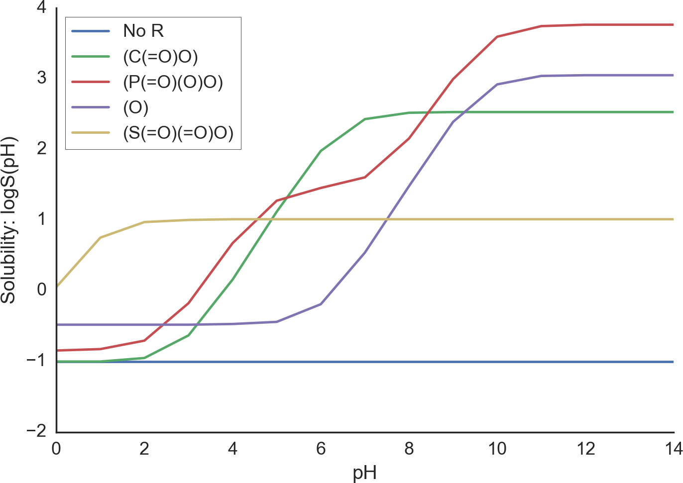
Figure 10: Predicted pH-dependent solubility of benzoquinones (BQ) with different functional groups. The legend describes R groups enumerated with BQ. Depending on pH, the solubility values of the quinones with a R-group significantly vary.

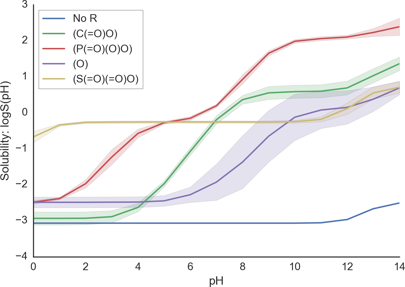
Figure 11: Predicted pH-dependent solubility of naphthoquinones (NQ) with different functional group substituents. Three unique positions are available to attach functional groups in NQ.

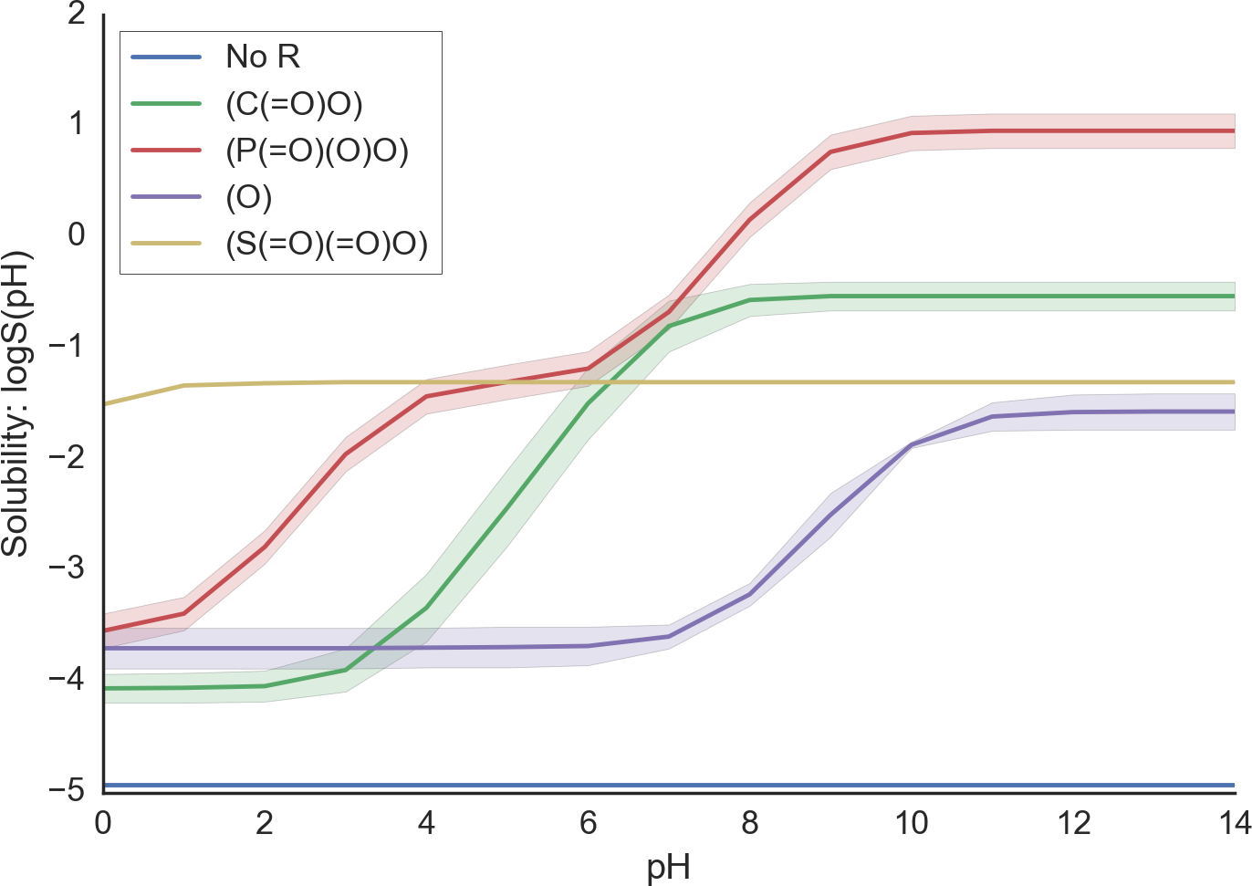
Figure 12: Predicted pH-dependent solubility of anthraquinone (AQ) with different functional group substituents. Two unique positions are available to attach functional groups in AQ.

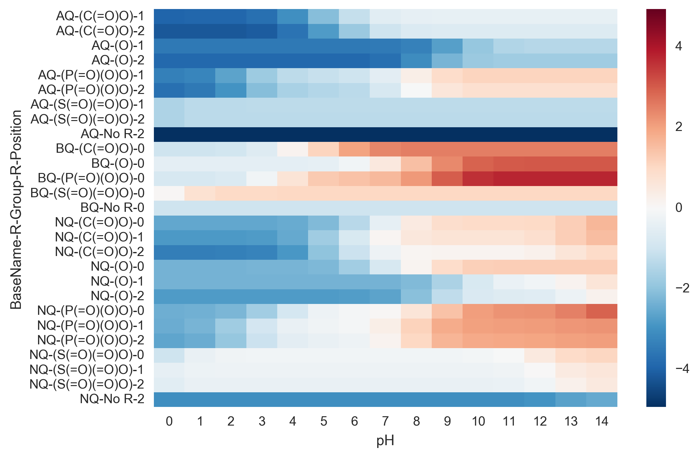
Figure 13: Heatmap of predicted pH-dependent solubility of all three quinone families with different functional group substituents.

3.2.3 pH-dependent solubility of multiple R-group anthraquinones

We predict the pH-dependent solubility of quinone molecules with multiple R-groups. Particularly, anthraquinone with multiple sulfonic acid groups and multiple hydroxyl groups are considered. Figure 14 shows structures of anthraquinones with zero, one, two and three sulfonic acid or hydroxyl groups. Quinone molecules with attached sulfonic acid group are particularly interesting since they display high solubilities and desirable redox potential values. In particular, 9,10-anthraquinone-2,7-disulphonic acid was chosen as a negative electrolyte ²⁵ and 1,2-dihydrobenzoquinone- 3,5-disulfonic acid was selected as a positive electrolyte ² for the acid quinoe flow batteries. The alkaline quinone flow battery embodies 2,6-dihydroxy-9,10-anthraquinone (2,6-DHAQ) as a negative electrolyte, and the experiment solubility of 2,6-DHAQ is reported as more than 0.6 M in 1 M KOH ³.

Figure 15 show that anthraquinone with no such R-groups is far insoluble in any pH condition while Table 4 picks solubility at pH 0, 7, 14 and includes prediction results by Chemaxon Cxcalc with logS plug-in as well as the extended MultiDK method. The MultiDK prediction shows that more sulfonic acid groups, more soluble, such as $P\log S_{\mathrm{pH}}$(AQTS) $>$ $P\log S_{\mathrm{pH}}$(AQDS) $>$ $P\log S_{\mathrm{pH}}$(AQS) $\gg$ $P\log S_{\mathrm{pH}}$(AQ), in all pH condition including the acid case and more hydroxyl groups, more soluble, such as $P\log S_{\mathrm{pH}}$(THAQ) $>$ $P\log S_{\mathrm{pH}}$(DHAQ) $>$ $P\log S_{\mathrm{pH}}$(HAQ) $\gg$ $P\log S_{\mathrm{pH}}$(AQ), in alkali condition. Therefore, it is noteworthy that an efficient prediction method should clearly differentiate between the solubility of an enumerated molecule according to the number of ionic functional groups in every pH points. The MultiDK with pH-dependent solubility estimation can be used as a more practical tool than the intrinsic solubility prediction method especially for the application of dicoverying organic flow battery electrodes.

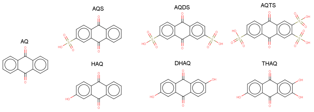
Figure 14: Anthraquinone and anthraquinone with either zero, mono-, di- and tetra-sulfonic acid or hydroxyl groups. Anthraquinone (AQ), anthraquinonesulfonic acid (AQS), anthraquinone-disulfonic acid (AQDS), anthraquinone-tetrasulfonic acid (AQTS), hydroxyl-anthraquinone (HAQ), dihydroxyl-anthraquinone (DHAQ) and tetrahydroxyl-anthraquinone (THAQ) are illustrated.

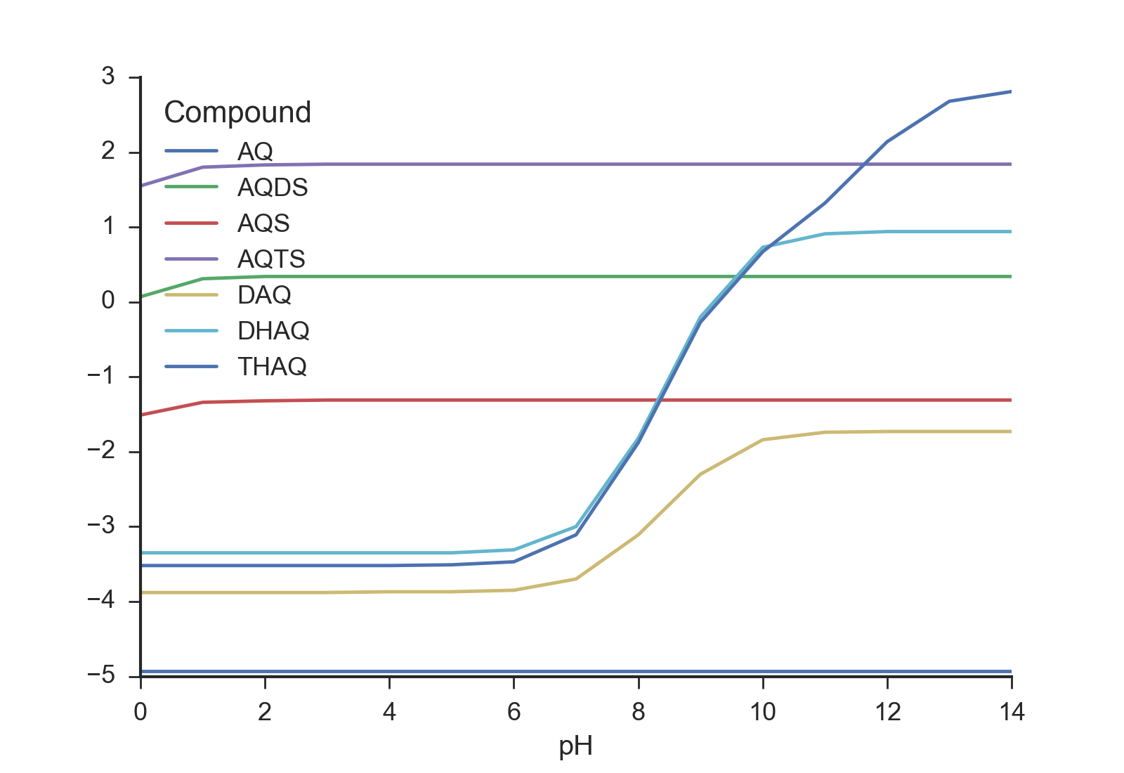
Figure 15: Predicted intrinsic and pH dependent solubility of seven anthraquinone family molecules with sulfonic or hydroxyl groups. Although their intrinsic solubility is predicted to have similar values, their pH-dependent solubility values are significantly varied depending on how many and which functional groups are attached.

Table 4: pH-dependent solubility of AQ with multiple R-groups where sulfonic acid and hydroxyl groups are considered. The pH-dependent solubility of them are estimated by MultDK and Chemaxon Cxcalc.

	MultiDK			Cxcalc
pH	0	7	14	0	7	14
AQ	-4.9	-4.9	-4.9	-4.5	-4.5	-4.5
AQS	-1.5	-1.3	-1.3	-1.6	0	0
AQDS	0.1	0.3	0.3	0	0	0
AQTS	1.6	1.8	1.8	0	0	0
HAQ	-3.9	-3.7	-1.7	-4.1	-3.9	0
DHAQ	-3.4	-3.0	0.9	-3.7	-3.3	0
THAQ	-3.5	-3.1	2.8	-3.3	-2.9	0

4 Conclusion

Organic aqueous flow battery systems require highly soluble electrolytes, which are two- to five-fold more soluble than pharmaceutical drugs. In order to search molecules with such a tight solubility requirement, high-throughput screening is a compelling approach especially when it is combined with an efficient solubility prediction method. Moreover, the investigation of pH-dependent solubility is essential to discovery highly soluble molecules which include an ionizable fragment such as the sulfonic acid (-SO₃H), the carboxylic acid (-COOH), the hydroxyl (-OH) and the dihydrogen phosphite (-PO₃H₂). We have developed a multiple descriptor multiple kernel (MultiDK) approach as an efficient property prediction method. As the ensemble descriptor consists of structure hash and fragment keys fingerprints as well as one or a few property specific descriptors such as molecular weight only or additionally Labute’s approximate surface area, and a partition coefficient, it has shown that MultiDK is capable of fast, accurate and universal solubility prediction. By the extension of MultiDK, the pH-dependent solubility of various quinones even with strong acidic or alkaline functional groups was investigated at each pH point where the quinones are the strong candidates of electrolytes for organic aqueous flow batteries.

5 Supplementary Information

5.1 MultiDK vs. SVR and DNN

The performance of support vector regression (SVR) and deep neural network (DNN) are tested for solubility estimation. The same descriptors to the cases of MultiDK23 are used for them. We evaluate SVR and DNN using the Scikit-learn and the Tensorflow packages in Python, respectively.

For SVR, we choose the kernel as radial basis function (RBF), which is given by

$$k_{\mathrm{RBF}}(\mathbf{x},\mathbf{y})=e^{\gamma|\mathbf{x}-\mathbf{y}|^{2}}$$ (5)

Penalty hyper parameter $C$ is searched for seven logarithmically equal spaced points from 1E-3 to 1E+3, while the other hyper parameter $\epsilon$ specifying the epsilon-tube and $\gamma$ are adjusted by the default values provided in the Scikit-learn package: $\epsilon=0.1$ and $\gamma=1/\mathrm{\#features}$. It is noteworthy that SVR requires a float point kernel computation for all descriptors regardless of a descriptor type while MultiDK computes binary kernel operation which obviously significantly faster than a float point computation. Figure 16 and Table 5 show that MultiDK outperforms RBF-SVR in all data set cases. Particularly, the average $r^{2}$ values of MultiDK and RBF-SVR are 0.87 and 0.83, respectively.

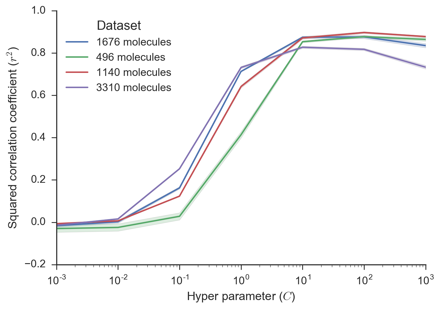
Figure 16: The $r^{2}$ distributions of SVR with respect to the hyper parameter of $C$.

Method	SVR			MultiDK
	Best $C$	E[$r^{2}$]	std($r^{2}$)	Best $\alpha$	E[$r^{2}$]	std($r^{2}$)
1676 molecules	1E+2	0.88	0.02	1E-1	0.91	0.03
496 molecules	1E+2	0.87	0.04	7E-2	0.89	0.05
1140 molecules	1E+2	0.90	0.01	3E-2	0.92	0.02
3310 molecules	1E+1	0.83	0.01	1E-1	0.87	0.04

Table 5: Average and std of the best $r^{2}$ values of SVR for each data set

For DNN, we evaluate the largest data set which includes the 3310 molecules. Also 20% of them are used for external testing while the 20% of the remained molecules are used for internal validation for DNN. We applied a lot of different network architectures manually and eventually find that a three hidden layer DNN with 100, 50, 10 weights for the first, second and third hidden layers shows the best performance among all our test structures. The performance of the best DNN is $r^{2}$=0.84, RMSE=0.86, MAE=0.60, DAE=0.42 for the test molecules, which is worse than the average $r^{2}$ of MultDK23 whereas DNN also employs the same descriptors to those of MultDK23, as aforementioned. The DAE represnts median absolute error.

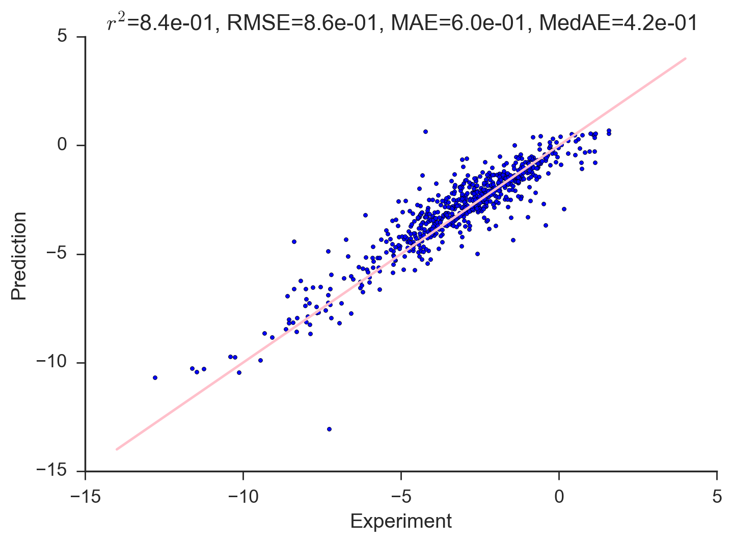
Figure 17: The experimental and predicted solubility of DNN for the test molecules are compared.

5.2 Kernels for a binary descriptor

The Tanimoto similarity has been used as a kernel function to exploit binary feature information such as recognizing white images on a black background. For further understanding, we compare the Tanimimoto similarity kernel with the linear kernel. The linear kernel is given by

$$k_{\mathrm{L}}(\mathbf{x},\mathbf{x}^{a}_{i})=\mathbf{x}^{T}\mathbf{x}^{a}_{i}=s$$ (6)

and the Tanimoto similarity kernel is given by

$$k_{\mathrm{T}}(\mathbf{x},\mathbf{x}^{a}_{i})=\frac{f_{\wedge}(\mathbf{x},\mathbf{x}^{a}_{i})}{f_{\vee}(\mathbf{x},\mathbf{x}^{a}_{i})}=\frac{s}{s+d}=\frac{1}{1+d/s}$$ (7)

where both $s=\mathbf{x}^{T}\mathbf{x}_{i}$ and $f_{\wedge}(\mathbf{x},\mathbf{x}^{a}_{i})=\sum_{j}x_{j}\wedge x^{a}_{i,j}=s$ are both the number of common 1’s in two vectors, $f_{\vee}(\mathbf{x},\mathbf{x}^{a}_{i})=\sum_{j}x_{j}\vee x^{a}_{i,j}$ is the number of 1’s in any two vectors and $d$ is equal to $f_{\vee}(\mathbf{x},\mathbf{x}^{a}_{i})-s$. The linear kernel of $k_{\mathrm{L}}(\mathbf{x},\mathbf{x}^{a}_{i})$ does not rely on $d$, while $k_{\mathrm{T}}(\mathbf{x},\mathbf{x}^{a}_{i})$ is inversely proportional to $d$ similar to a characteristic of the radial basis function. Therefore, a kernel regression with $k_{\mathrm{T}}(\mathbf{x},\mathbf{x}^{a}_{i})$, the Tanimoto similarity, can offer better performance than the linear kernel regression as shown in the main text, refering to MD versus MultiDK.

References

- Huskinson et al. 2014 Huskinson, B.; Marshak, M. P.; Suh, C.; Er, S.; Gerhardt, M. R.; Galvin, C. J.; Chen, X.; Aspuru-Guzik, A.; Gordon, R. G.; Aziz, M. J. Nature 2014, 505, 195–198
- Yang et al. 2014 Yang, B.; Hoober-Burkhardt, L.; Wang, F.; Prakash, G. K. S.; Narayanan, S. R. Journal of The Electrochemical Society 2014, 161, A1371–A1380, 00000
- Lin et al. 2015 Lin, K.; Chen, Q.; Gerhardt, M. R.; Tong, L.; Kim, S. B.; Eisenach, L.; Valle, A. W.; Hardee, D.; Gordon, R. G.; Aziz, M. J.; Marshak, M. P. Science 2015, 349, 1529–1532
- Liu et al. 2016 Liu, T.; Wei, X.; Nie, Z.; Sprenkle, V.; Wang, W. Advanced Energy Materials 2016, 6, 1501449
- Winsberg et al. 2016 Winsberg, J.; Janoschka, T.; Morgenstern, S.; Hagemann, T.; Muench, S.; Hauffman, G.; Gohy, J.-F.; Hager, M. D.; Schubert, U. S. Advanced Materials 2016, 28, 2238–2243
- Soloveichik 2015 Soloveichik, G. L. Chemical Reviews 2015, 115, 11533–11558, PMID: 26389560
- Yang et al. 2016 Yang, B.; Hoober-Burkhardt, L.; Krishnamoorthy, S.; Murali, A.; Prakash, G. K. S.; Narayanan, S. R. Journal of The Electrochemical Society 2016, 163, A1442–A1449
- Pyzer-Knapp et al. 2016 Pyzer-Knapp, E. O.; Simm, G. N.; Aspuru-Guzik, A. Materials Horizons 2016, 3, 226–233
- Plessow et al. 2016 Plessow, P. N.; Bajdich, M.; Greene, J.; Vojvodic, A.; Abild-Pedersen, F. The Journal of Physical Chemistry C 2016, 120, 10351–10360
- Peplow 2015 Peplow, M. Nature News 2015, 520, 148
- Santos et al. 2016 Santos, E. J. G.; Nørskov, J. K.; Vojvodic, A. The Journal of Physical Chemistry C 2016, 119, 17662–17666
- Ma et al. 2015 Ma, J.; Sheridan, R. P.; Liaw, A.; Dahl, G. E.; Svetnik, V. Journal of Chemical Information and Modeling 2015, 55, 263–274
- Shu and Levine 2015 Shu, Y.; Levine, B. G. The Journal of Chemical Physics 2015, 142, 104104
- Hachmann et al. 2014 Hachmann, J.; Olivares-Amaya, R.; Jinich, A.; Appleton, A. L.; Blood-Forsythe, M. A.; Seress, L. R.; Román-Salgado, C.; Trepte, K.; Atahan-Evrenk, S.; Er, S.; Shrestha, S.; Mondal, R.; Sokolov, A.; Bao, Z.; Aspuru-Guzik, A. Energy & Environmental Science 2014, 7, 698–704
- Curtarolo et al. 2013 Curtarolo, S.; Hart, G. L. W.; Nardelli, M. B.; Mingo, N.; Sanvito, S.; Levy, O. Nature Materials 2013, 12, 191–201
- Kanal et al. 2013 Kanal, I. Y.; Owens, S. G.; Bechtel, J. S.; Hutchison, G. R. The Journal of Physical Chemistry Letters 2013, 4, 1613–1623
- Sokolov et al. 2011 Sokolov, A. N.; Atahan-Evrenk, S.; Mondal, R.; Akkerman, H. B.; Sánchez-Carrera, R. S.; Granados-Focil, S.; Schrier, J.; Mannsfeld, S. C. B.; Zoombelt, A. P.; Bao, Z.; Aspuru-Guzik, A. Nature Communications 2011, 2, 437
- Fischer et al. 2006 Fischer, C. C.; Tibbetts, K. J.; Morgan, D.; Ceder, G. Nature Materials 2006, 5, 641–646
- Shoichet 2004 Shoichet, B. K. Nature 2004, 432, 862–865
- Bajorath 2002 Bajorath, J. Nature Reviews Drug Discovery 2002, 1, 882–894
- Er et al. 2015 Er, S.; Suh, C.; Marshak, M. P.; Aspuru-Guzik, A. Chem. Sci. 2015, 6, 885–893
- Pineda Flores et al. 2015 Pineda Flores, S. D.; Martin-Noble, G. C.; Phillips, R. L.; Schrier, J. The Journal of Physical Chemistry C 2015, 119, 21800–21809
- Wang and Hou 2011 Wang, J.; Hou, T. Combinatorial chemistry & high throughput screening 2011, 14, 328–338, 00036
- Skyner et al. 2015 Skyner, R. E.; McDonagh, J. L.; Groom, C. R.; Mourik, T. v.; Mitchell, J. B. O. Physical Chemistry Chemical Physics 2015, 17, 6174–6191, 00001
- Huuskonen 2000 Huuskonen, J. Journal of Chemical Information and Computer Sciences 2000, 40, 773–777
- Bhal et al. 2007 Bhal, S. K.; Kassam, K.; Peirson, I. G.; Pearl, G. M. Molecular Pharmaceutics 2007, 4, 556–560
- Bergström et al. 2004 Bergström, C. A. S.; Luthman, K.; Artursson, P. European Journal of Pharmaceutical Sciences 2004, 22, 387–398, 00000
- Mitchell 2014 Mitchell, J. B. O. Wiley Interdisciplinary Reviews: Computational Molecular Science 2014, 4, 468–481, 00011
- Hughes et al. 2008 Hughes, L. D.; Palmer, D. S.; Nigsch, F.; Mitchell, J. B. O. Journal of Chemical Information and Modeling 2008, 48, 220–232, 00085
- Palmer et al. 2007 Palmer, D. S.; O’Boyle, N. M.; Glen, R. C.; Mitchell, J. B. O. Journal of Chemical Information and Modeling 2007, 47, 150–158, 00000
- McDonagh et al. 2014 McDonagh, J. L.; Nath, N.; De Ferrari, L.; van Mourik, T.; Mitchell, J. B. O. Journal of Chemical Information and Modeling 2014, 54, 844–856, 00000
- Marten et al. 1996 Marten, B.; Kim, K.; Cortis, C.; Friesner, R. A.; Murphy, R. B.; Ringnalda, M. N.; Sitkoff, D.; Honig, B. The Journal of Physical Chemistry 1996, 100, 11775–11788
- Tannor et al. 1994 Tannor, D. J.; Marten, B.; Murphy, R.; Friesner, R. A.; Sitkoff, D.; Nicholls, A.; Honig, B.; Ringnalda, M.; Goddard, W. A. Journal of the American Chemical Society 1994, 116, 11875–11882
- Raccuglia et al. 2016 Raccuglia, P.; Elbert, K. C.; Adler, P. D. F.; Falk, C.; Wenny, M. B.; Mollo, A.; Zeller, M.; Friedler, S. A.; Schrier, J.; Norquist, A. J. Nature 2016, 533, 73–76
- Silver et al. 2016 Silver, D. et al. Nature 2016, 529, 484–489
- Jain and Yalkowsky 2001 Jain, N.; Yalkowsky, S. H. Journal of Pharmaceutical Sciences 2001, 90, 234–252
- Ran et al. 2002 Ran, Y.; He, Y.; Yang, G.; Johnson, J. L. H.; Yalkowsky, S. H. Chemosphere 2002, 48, 487–509
- Delaney 2004 Delaney, J. S. Journal of Chemical Information and Computer Sciences 2004, 44, 1000–1005
- Wang et al. 2009 Wang, J.; Hou, T.; Xu, X. Journal of Chemical Information and Modeling 2009, 49, 571–581, PMID: 19226181
- Tetko and Bruneau 2004 Tetko, I. V.; Bruneau, P. Journal of Pharmaceutical Sciences 2004, 93, 3103–3110
- Tetko et al. 2001 Tetko, I. V.; Tanchuk, V. Y.; Villa, A. E. P. Journal of Chemical Information and Computer Sciences 2001, 41, 1407–1421, 00288
- Lipinski et al. 2001 Lipinski, C. A.; Lombardo, F.; Dominy, B. W.; Feeney, P. J. Advanced Drug Delivery Reviews 2001, 46, 3–26, 00000
- Viswanadhan et al. 1989 Viswanadhan, V. N.; Ghose, A. K.; Revankar, G. R.; Robins, R. K. Journal of Chemical Information and Computer Sciences 1989, 29, 163–172
- Ali et al. 2012 Ali, J.; Camilleri, P.; Brown, M. B.; Hutt, A. J.; Kirton, S. B. Journal of Chemical Information and Modeling 2012, 52, 420–428
- Zhou et al. 2008 Zhou, D.; Alelyunas, Y.; Liu, R. Journal of Chemical Information and Modeling 2008, 48, 981–987
- Durant et al. 2002 Durant, J. L.; Leland, B. A.; Henry, D. R.; Nourse, J. G. Journal of Chemical Information and Computer Sciences 2002, 42, 1273–1280
- Klopman et al. 1992 Klopman, G.; Wang, S.; Balthasar, D. M. Journal of Chemical Information and Computer Sciences 1992, 32, 474–482, 00000
- Kühne et al. 1995 Kühne, R.; Ebert, R. U.; Kleint, F.; Schmidt, G.; Schüürmann, G. Chemosphere 1995, 30, 2061–2077
- Cheng et al. 2011 Cheng, T.; Li, Q.; Wang, Y.; Bryant, S. H. Journal of Chemical Information and Modeling 2011, 51, 229–236, 00019
- Tetko and Poda 2004 Tetko, I. V.; Poda, G. I. Journal of Medicinal Chemistry 2004, 47, 5601–5604
- Xing and Glen 2002 Xing, L.; Glen, R. C. Journal of Chemical Information and Computer Sciences 2002, 42, 796–805
- Hall and Kier 1995 Hall, L. H.; Kier, L. B. Journal of Chemical Information and Computer Sciences 1995, 35, 1039–1045
- Rogers and Hahn 2010 Rogers, D.; Hahn, M. Journal of Chemical Information and Modeling 2010, 50, 742–754
- Duvenaud et al. 2015 Duvenaud, D. K.; Maclaurin, D.; Iparraguirre, J.; Bombarell, R.; Hirzel, T.; Aspuru-Guzik, A.; Adams, R. P. In Advances in Neural Information Processing Systems 28; Cortes, C., Lawrence, N. D., Lee, D. D., Sugiyama, M., Garnett, R., Eds.; Curran Associates, Inc., 2015; pp 2224–2232
- Lind and Maltseva 2003 Lind, P.; Maltseva, T. Journal of Chemical Information and Computer Sciences 2003, 43, 1855–1859, PMID: 14632433
- Steinbeck et al. 2006 Steinbeck, C.; Hoppe, C.; Kuhn, S.; Floris, M.; Guha, R.; Willighagen, E. L. Current Pharmaceutical Design 2006, 12, 2111–2120
- Efron et al. 2004 Efron, B.; Hastie, T.; Johnstone, I.; Tibshirani, R.; others, The Annals of statistics 2004, 32, 407–499
- Hou et al. 2004 Hou, T. J.; Xia, K.; Zhang, W.; Xu, X. J. Journal of Chemical Information and Computer Sciences 2004, 44, 266–275
- Ledwidge and Corrigan 1998 Ledwidge, M. T.; Corrigan, O. I. International Journal of Pharmaceutics 1998, 174, 187–200
- Hansen et al. 2006 Hansen, N. T.; Kouskoumvekaki, I.; Jørgensen, F. S.; Brunak, S.; Jónsdóttir, S. Ó. Journal of Chemical Information and Modeling 2006, 46, 2601–2609, 00000
- Wang et al. 2015 Wang, J.-B.; Cao, D.-S.; Zhu, M.-F.; Yun, Y.-H.; Xiao, N.; Liang, Y.-Z. Journal of Chemometrics 2015, 29, 389–398, 00000
- Pyzer-Knapp et al. 2015 Pyzer-Knapp, E. O.; Suh, C.; Gómez-Bombarelli, R.; Aguilera-Iparraguirre, J.; Aspuru-Guzik, A. Annual Review of Materials Research 2015, 45, 195–216
- Kearnes et al. 2014 Kearnes, S. M.; Haque, I. S.; Pande, V. S. Journal of chemical information and modeling 2014, 54, 5–15
- Wang et al. 2007 Wang, J.; Krudy, G.; Hou, T.; Zhang, W.; Holland, G.; Xu, X. Journal of Chemical Information and Modeling 2007, 47, 1395–1404
- Willighagen et al. 2006 Willighagen, E. L.; Denissen, H. M. G. W.; Wehrens, R.; Buydens, L. M. C. Journal of Chemical Information and Modeling 2006, 46, 487–494, PMID: 16562976
- McKinney 2010 McKinney, W. Data Structures for Statistical Computing in Python. Proceedings of the 9th Python in Science Conference. 2010; pp 51 – 56
- Pedregosa et al. 2011 Pedregosa, F. et al. Journal of Machine Learning Research 2011, 12, 2825–2830
- Abadi et al. 2015 Abadi, M. et al. TensorFlow: Large-Scale Machine Learning on Heterogeneous Systems. 2015; http://tensorflow.org/, Software available from tensorflow.org
- Waskom et al. 2016 Waskom, M. et al. seaborn: v0.7.0 (January 2016). 2016; http://dx.doi.org/10.5281/zenodo.45133
- Gönen and Alpaydin 2011 Gönen, M.; Alpaydin, E. The Journal of Machine Learning Research 2011, 12, 2211–2268
- Bach et al. 2004 Bach, F. R.; Lanckriet, G. R. G.; Jordan, M. I. Multiple Kernel Learning, Conic Duality, and the SMO Algorithm. Proceedings of the Twenty-first International Conference on Machine Learning. 2004
- Lanckriet et al. 2014 Lanckriet, G. R.; Cristianini, N.; Bartlett, P.; Ghaoui, L. E.; Jordan, M. I. The Journal of Machine Learning Research 2014, 5, 27–72
- Yu et al. 2010 Yu, S.; Falck, T.; Daemen, A.; Tranchevent, L.-C.; Suykens, J. A.; Moor, B. D.; Moreau, Y. BMC Bioinformatics 2010, 11, 309
- Chen et al. 2013 Chen, L.; Duan, L.; Xu, D. Event Recognition in Videos by Learning from Heterogeneous Web Sources. 2013 IEEE Conference on Computer Vision and Pattern Recognition (CVPR). 2013; pp 2666–2673
- Xu et al. 2013 Xu, X.; Tsang, I. W.; Xu, D. IEEE transactions on neural networks and learning systems 2013, 24, 749–761
- Pekalska et al. 2001 Pekalska, E.; Paclik, P.; Duin, R. P. W. J. Machine Learning Res. 2001, 175–211
- Kew and Mitchell 2015 Kew, W.; Mitchell, J. B. O. Molecular Informatics 2015, 34, 634–647
- rdk 2015 RDKit: Open-source cheminformatics. http://www.rdkit.org, 2015; [Online; version 2-September-2015]
- cxc 1998-2009 Calculator Plugins (Cxcalc) were used for structure property prediction and calculation, Marvin 5.2.2, Chemaxon. ChemAxon(http://www.chemaxon.com), 1998-2009
- Buitinck et al. 2013 Buitinck, L.; Louppe, G.; Blondel, M.; Pedregosa, F.; Mueller, A.; Grisel, O.; Niculae, V.; Prettenhofer, P.; Gramfort, A.; Grobler, J.; Layton, R.; VanderPlas, J.; Joly, A.; Holt, B.; Varoquaux, G. API design for machine learning software: experiences from the scikit-learn project. ECML PKDD Workshop: Languages for Data Mining and Machine Learning. 2013; pp 108–122
- Sijm et al. 1999 Sijm, D. T. H. M.; Schüürmann, G.; de Vries, P. J.; Opperhuizen, A. Environmental Toxicology and Chemistry 1999, 18, 1109–1117
- che 2015 Chemicalize.org was used for name to structure generation/prediction of xyz properties/etc, Chemaxon. chemicalize.org, 2015; Accessed: 2015-10-06
- Labute 2000 Labute, P. Journal of Molecular Graphics and Modelling 2000, 18, 464–477
- Tetko et al. 2001 Tetko, I. V.; Tanchuk, V. Y.; Kasheva, T. N.; Villa, A. E. P. Journal of Chemical Information and Computer Sciences 2001, 41, 1488–1493, 00244