Transient cell assembly networks encode persistent spatial memories

Abstract

While cognitive representations of an environment can last for days and even months, the synaptic architecture of the neuronal networks that underlie these representations constantly changes due to various forms of synaptic and structural plasticity at a much faster timescale. This raises an immediate question: how can a transient network maintain a stable representation of space? In the following, we propose a computational model for describing emergence of the hippocampal cognitive map ina network of transient place cell assemblies and demonstrate, using methods of algebraic topology, that such a network can maintain a robust map of the environment.

I Introduction

The mammalian hippocampus plays a major role in spatial cognition, spatial learning and spatial memory by producing an internalized representation of space—a cognitive map of the environment Tolman ; OKeefe ; Nadel ; McNaughton . Several key observations shed light on the neuronal computations responsible for implementing such a map. The first observation is that the spiking activity of the principal cells in the hippocampus is spatially tuned. In rats, these neurons, called place cells, fire only in restricted locations—their respective place fields Best1 . As demonstrated in many studies, this simple principle allows decoding the animal’s ongoing trajectory Brown1 ; Guger , its past navigational experience Carr , and even its future planned routs Pfeiffer ; Dragoi1 ; Dragoi2 from the place cell’s spiking activity.

The second observation is that the spatial layout of the place fields—the place field map—is “flexible”: as the environment is deformed, the place fields shift and change their shapes, while preserving most of their mutual overlaps, adjacency and containment relationships Gothard ; Leutgeb ; Wills ; Touretzky . Thus, the sequential order of place cells’ (co)activity induced by the animal’s moves through morphing environment remains invariant within a certain range of geometric transformations Diba ; eLife ; Alvernhe ; Poucet ; Wu . This implies that the place cells’ spiking encodes a coarse framework of qualitative spatiotemporal relationships, i.e., that the hippocampal map is topological in nature, more similar to a schematic subway map than to a topographical city map eLife .

The third observation concerns the synaptic architecture of the (para)hippocampal network: it is believed that groups of place cells that demonstrate repetitive coactivity form functionally interconnected “assemblies,” which together drive their respective “reader-classifier” or “readout” neurons in the downstream networks Harris1 ; Buzsaki1 . The activity of a readout neuron actualizes the qualitative relationships between the regions encoded by the individual place cells, thus defining the type of spatial connectivity information encoded in the hippocampal map Schemas .

A given cell assembly network architecture appears as a result of spatial learning, i.e., it emerges from place cell coactivities produced during an animal’s navigation through a particular place field map, via a “fire-together-wire-together” plasticity mechanism Caroni ; Chklovskii . However, a principal property of the cell assemblies is that they may not only form, but also or disband as a result of a depression of synapses caused by reduction or cessation of spiking activity over a sufficiently long timespan Wang . Some of the disbanded cell assemblies may later reappear during a subsequent period of coactivity, then disappear again, and so forth. Electrophysiological studies suggest that the lifetime of the cell assemblies ranges between minutes Kuhl ; Murre to hundreds of milliseconds Atallah ; Bartos ; Mann ; Whittington ; Bi . In contrast, spatial memories in rats can last much longer Meck ; Clayton ; Brown2 , raising the question: how can a large-scale spatial representation of the environment be stable if the neuronal stratum that computes this representation changes on a much faster timescale?

The hypothesis that the hippocampus encodes a topological map of the environment allows this question to be addressed computationally. Below, we propose a phenomenological model of a transient hippocampal network and use methods of algebraic topology to demonstrate that a large-scale topological representation of the environment encoded by this network may remain stable despite the transience of neuronal connections.

II The Model

In PLoS ; Arai , we proposed a computational approach to integrating the information provided by the individual place cells into a large-scale topological representation of the environment, based on several remarkable parallels between the elements of hippocampal physiology and certain notions of algebraic topology. There, we regarded a particular collection of coactive place cells $c_{1}$, $c_{2}$, …, $c_{n}$ as an abstract “coactivity simplex” $\sigma=[c_{1},c_{2},...,c_{n}]$, which may be visualized (for $n\leq 4$) or apprehended (for $n\geq 5$) as an $(n-1)$-dimensional polyhedron Aleksandrov . As a result, the pool of coactivities is represented by a simplicial “coactivity” complex $\mathcal{T}$, which provides a link between the cellular and the net systemic level of the information processing. Just like simplexes, the individual cell groups provide local information about the environment, but together, as a neuronal ensemble, they represent space as whole—as the simplicial complex. Numerical experiments PLoS ; Arai ; Curto backed up by a remarkable theorem due to P. Alexandrov Alexandroff and E. Čech’s Cech point out that $\mathcal{T}$ correctly represents the topological structure of the rat’s environment and may serve as a schematic model of the hippocampal map Schemas . For example, the paths traveled by the rat are represented by the “simplicial paths”—chains of simplexes in $\mathcal{T}$ that capture certain qualitative properties of their physical counterparts (see Dabaghian1 ; Novikov and Fig. 1A).

Of course, producing a faithful representation of the environment from place cell coactivity requires learning. In the model, this process is represented by the dynamics of the coactivity complex’s formation. At every moment of time, the coactivity complex represents only those place cell combinations that have exhibited (co)activity. As the animal begins to explore the environment, the newly emerging coactivity complex is small, fragmented and contains many holes, most of which do not correspond to physical obstacles or to the regions that have not yet been visited by the animal. These “spurious” structures tend to disappear as the pool of place cell coactivities accumulates. Numerical simulations show that, if place cells operate within biological parameters PLoS , the topological structure of $\mathcal{T}$ becomes equivalent to the topological stricture of the environment within minutes. The minimal time $T_{\min}$ required to produce a correct topological representation of the environment can be used as an estimate for the time required to learn spatial connectivity (Fig. 1B, PLoS ; Arai ; Curto ).

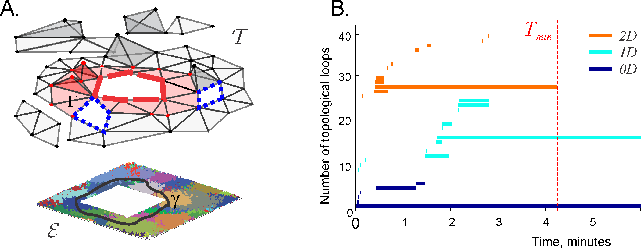
Figure 1: Schematic representation of place cell coactivity in the cell assembly complex $\mathcal{T}$. (A) Bottom: Simulated place map covering a small planar environment $\mathcal{E}$ that contains a square hole in the middle. The clusters of colored dots represent the place fields, and a typical path traversed by the animal is shown by the black loop $\gamma$. The coactivity complex $\mathcal{T}$ induced from the coactivity of the place cells (on the top) provides a topological representation of environment. The hole in the middle of $\mathcal{T}$ (red dashed line) corresponds to the central hole in the environment $\mathcal{E}$. The non-contractible closed chain of simplexes—a simplicial path $\Gamma$—corresponds to the non-contractible physical path $\gamma$. In general, the complex can be fragmented in pieces and contain gaps (holes encircled by blue loops), which represent topological noise, rather than information about the environment. (B) Timelines of zero-dimensional ($0D$), one-dimensional ($1D$) and two-dimensional ($2D$) topological loops encoded in a coactivity complex $\mathcal{T}$ which represents the environment $\mathcal{E}$. For as long as a given $0D$ loop persists, it indicates that the coactivity complex contains the corresponding connectivity component. A persisting $1D$ loop represents a noncontractible hole in $\mathcal{T}$ (see red hole in $\mathcal{T}$ on the left panel). A persistent $2D$ loop represents a noncontractible $2D$ sphere in $\mathcal{T}$. In the illustrated case, the $0D$ spurious loops disappear in about 1.5 minutes, indicating that the coactivity complex $\mathcal{T}$ fuses into one piece at that time. The $1D$ spurious disappear when all the spurious holes in $\mathcal{T}$ close up in about 2.8 min, and the $2D$ loops disappear by $T_{\min}=4.2$ min (dashed vertical line), at which point the topology of $\mathcal{T}$ becomes equivalent to the topology of the environment.

Coactivity complexes. A specific algorithm used to implement a coactivity complex may be designed to incorporate physiological information about place cell cofiring at different levels of detail. In the simplest case, every observed group of coactive place cells contributes a simplex; the resulting coactivity complex $\mathcal{T}$ (referred to as the Čech coactivity complex in PLoS ; Arai ) makes no reference to the structure of the hippocampal network or to the cell assemblies, and gives a purely phenomenological description of the information contained in the place cell coactivity. In a more detailed approach, the maximal simplexes of the coactivity complex (i.e., the simplexes that are not subsimplexes of any larger simplex) may be selected to represent ignitions of the place cell assemblies, rather than arbitrary place cell combinations. The combinatorial arrangement of the maximal simplexes in the resulting “cell assembly coactivity complex,” denoted $\mathcal{T}_{CA}$, schematically represents the network of interconnected cell assemblies Schemas ; Babichev1 (Fig. 2A).

The specific algorithm of constructing the complex $\mathcal{T}_{CA}$ may also reflect how neuronal coactivity is processed by the readout neurons. If these neurons function as “coincidence detectors,” i.e., if they react to the spikes received within a short coactivity detection period $w$ (typically, $w\approx 200-250$ milliseconds Arai ; Mizuseki ), then the maximal simplexes in the corresponding coincidence detection coactivity complex (denoted $\mathcal{T}_{\ast}$) will appear instantaneously at the moments of the cell assemblies’ ignitions Babichev1 ; Hoffmann . Alternatively, if the readout neurons integrate the coactivity inputs from smaller parts of their respective assemblies over an extended coactivity integration period $\varpi$ Konig ; Ratte , then the appearance of the maximal simplexes in the corresponding input integration coactivity complex (denoted as $\mathcal{T}_{+})$ will extend over time, reflecting the dynamics of synaptic integration. The time course of the maximal simplexes’ appearance affects the rate at which large-scale topological information is accumulated and hence controls the model’s description of spatial learning.

Computational implementation of the coactivity complexes $\mathcal{T}_{\ast}$ and $\mathcal{T}_{+}$ is as follows. The maximal simplexes of the coincidence detection coactivity complex $\mathcal{T}_{\ast}$ are selected from the pool of the most frequently appearing groups of simultaneously coactive place cells Babichev1 . To model an input integrator coactivity complex $\mathcal{T}_{+}$, we first built a connectivity graph $G$ that represents pairwise place cell coactivities observed within a certain period $\varpi$. Then we build the associated clique complex $\mathcal{T}_{\varsigma}(G)$, i.e., we view the maximal, fully interconnected subgraphs of the graph $G$, which are its cliques $\varsigma$, as simplexes of $\mathcal{T}_{\varsigma}$ (for details see Methods in Babichev1 and Jonsson ). The process of assembling the fully interconnected cliques from pairwise connections is designed to model the process of integrating the spiking inputs in the cell assemblies, so that the resulting clique coactivity complex $\mathcal{T}_{\varsigma}$ serves as a model of the input integration cell assembly network.

Numerical simulations show that, for a given population of place cells, the clique complex $\mathcal{T}_{\varsigma}$ is typically larger and forms faster than the coincidence detector (Čech) complex $\mathcal{T}_{\varsigma}$, and, as a result, $\mathcal{T}_{\varsigma}$ reproduces the topological structure of the environment more reliably Schemas ; Babichev1 . Moreover, the coincidence detection coactivity complexes can be viewed as a specific case of the input integration coactivity complexes: as the integration period shrinks and approaches the coactivity period $\varpi\to w$, the input integration coactivity complex $\mathcal{T}_{\varsigma}$ reduces to the coincidence complex $\mathcal{T}_{\varsigma}$. For these reasons, in the following we will model only the input integration, i.e., clique coactivity complexes.

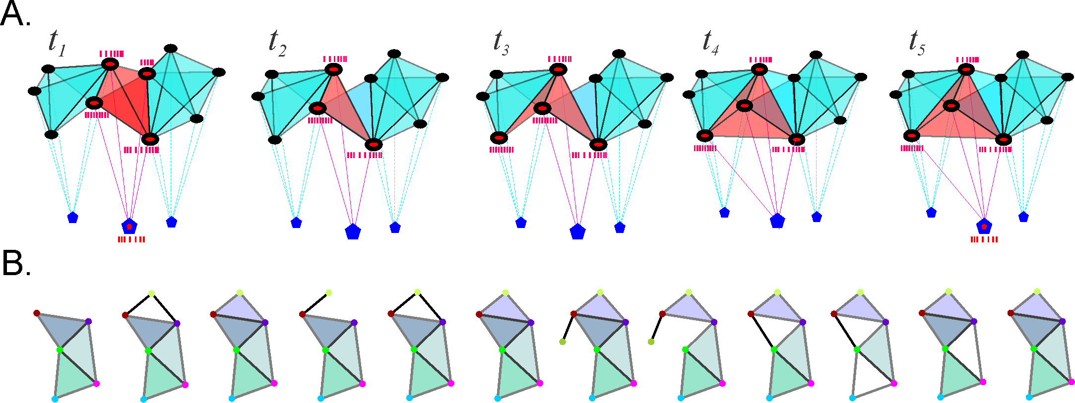
Figure 2: Place cell assemblies and flickering coactivity complexes. (A) Functionally interconnected groups of place cells (place cell assemblies) are schematically represented by fully interconnected cliques. The place cells (small disks) in a given assembly $\varsigma$ are synaptically connected to the corresponding readout neuron $n_{\varsigma}$ (pentagons below). An assembly $\varsigma$ ignites (red clique/tetrahedron in the middle) when its place cells elicit jointly a spiking response from the readout neuron $n_{\varsigma}$ (active cells have red centers). A cell assembly may be active at a certain moment of time, then disactivate, then become active again, and so forth. If a certain cell assembly ceases to ignite and another combination of place cells begins to exhibit frequent coactivity, the old cell assembly is replaced by new one. (B) The formation and disbanding of the cell assemblies is schematically represented in the “flickering” coactivity complex, in which the maximal simplexes appear and disappear, representing appearance and disappearance of the cell assemblies in the hippocampal network.

Instability of the cell assemblies. In our previous work Babichev1 , the frequencies of the cell assemblies’ appearances, $f_{\varsigma}$, were computed across the entire navigation period $T_{tot}$, i.e., the cell assemblies were presumed to exist from the moment of their first appearance for as long as the navigation continued. In order to model cell assemblies with finite lifetimes, these frequencies should be evaluated within shorter periods $\varpi_{\varsigma}<T_{tot}$. Physiologically, $\varpi_{\varsigma}$ can be viewed as the period during which the readout neuron $n_{\varsigma}$ may connect synaptically to a particular combination of coactive place cells, i.e., form a cell assembly $\varsigma$, retain these connections, and respond to subsequent ignitions of $\varsigma$. In a population of cell assemblies, the integration periods can be distributed with a certain mode $\varpi$ and a variance $\Delta_{\varpi}$. However, in order to simplify the approach, we will make two assumptions. First, we will describe the entire population of the readout neurons in terms of the integration period of a typical readout neuron, i.e., describe the ensemble of readout neurons with a single parameter, $\varpi$. Second, we will assume that the integration periods of all neurons are synchronized, i.e., that there exists a globally defined coactivity integration window of width $\varpi$ during which the entire population of the readout neurons synchronously processes coactivity inputs from their respective place cell assemblies. In such case, $\varpi$ can be viewed as a period during which the cell assembly network processes the ongoing place cell spiking activity. Below we demonstrate that these restrictions result in a simple model that allows describing a population of finite lifetime cell assemblies and show that the resulting cell assembly network, for a sufficiently large $\varpi$, reliably encodes the topological connectivity of the environment.

Computational model of the transient cell assembly network. A network of rewiring cell assemblies is represented by a coactivity complex with fluctuating or “flickering” maximal simplexes. To build such a complex, denoted $\mathcal{F}$, we implement a “sliding coactivity integration window” approach. First, we identify the maximal simplexes that emerge within the first $\varpi$-period after the onset of the navigation $\varpi_{1}$ based on the place cell activity rates evaluated within that window, $f_{\varsigma}(\varpi_{1})$, and construct the corresponding input integration coactivity complex $\mathcal{F}(\varpi_{1})$. Then the algorithm is repeated for the subsequent windows $\varpi_{2}$, $\varpi_{3}$,… which are obtained by shifting the starting window $\varpi_{1}$ over small time steps $\Delta t$. Since consecutive windows overlap, the corresponding coactivity complexes $\mathcal{F}(\varpi_{2})$, $\mathcal{F}(\varpi_{2})$, … consist of overlapping sets of maximal simplexes. A given maximal simplex $\varsigma$ (defined by the set of its vertexes) may appear in a chain of consecutive windows $\varpi_{1}$, $\varpi_{2}$, …, $\varpi_{k-1}$ then disappear at a step $\varpi_{k}$ (i.e., $\varsigma\in\mathcal{F}(\varpi_{k-1}$), but $\varsigma\notin\mathcal{F}(\varpi_{k})$), then reappear in a later window $\varpi_{l}$, then disappear again, and so forth (Fig. 2). The midpoint $t_{k}$ of the window in which the maximal simplex $\varsigma$ has (re)appeared defines the moment of $\varsigma$’s (re)birth, and the midpoints of the windows were is disappears, are viewed as the times of its deaths. Indeed, one may use the left or the right end of the shifting integration window, which would affect the endpoints of the navigation, but not the net results discussed below. As a result, the lifetime $\delta t_{\varsigma,k}$ of a cell assembly $\varsigma$ between its $k$-th consecutive appearance and disappearance can be as short as $\Delta t$ (if $\varsigma$ appears within $\varpi_{k}$ and disappears at the next step, within $\varpi_{k+1}$, or as long as $T_{tot}$ - $\varpi$ in the case that $\varsigma$ appears at the first step and never disappears. However, a typical maximal simplex exhibits a spread of lifetimes that can be characterized by a half-life, as we will discuss below.

It is natural to view the coactivity complexes $\mathcal{F}(\varpi_{i})$ as instances of a single flickering coactivity complex $\mathcal{F}_{\varpi}$, $\mathcal{F}_{\varpi}(t_{i})=\mathcal{F}(\varpi_{i})$, having appearing and disappearing maximal simplexes (see Fig. 2B and Babichev2 ). In the following, we will use $\mathcal{F}_{\varpi}$ as a model of transient cell assembly network and study whether such a network can encode a stable topological map of the environment on the moment-by-moment basis.

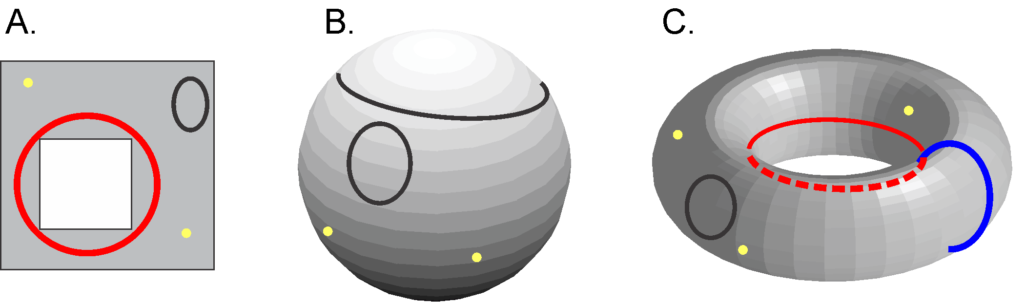
Figure 3: Topological shapes defined in terms of topological loops. (A) Any two zero-dimensional ($0D$) loops (i.e., points, yellow dots) in the two-dimensional space $\mathcal{E}$ navigated by the simulated rat (see Fig. 1A) can be matched with one another via continuous moves. This implies that all $0D$ loops are topologically equivalent to a single “representative” loop, i.e., that zeroth Betti number of $\mathcal{E}$ is $b_{0}(\mathcal{E})=1$. The one-dimensional ($1D$) loops are of two types: some contract to a point (e.g., the black loop in the corner) and others (e.g., the red loop in the middle) are non-contractible, signaling the existence of a topological obstruction—the central hole, which is the main topological feature of $\mathcal{E}$. Thus, $b_{1}(\mathcal{E})=1$. Since the entire space $\mathcal{E}$ can be contracted to the $1D$ rim of the central hole, there are no higher dimensional noncontractible topological loops in $\mathcal{E}$, $b_{n>1}(\mathcal{E})=0$. The net barcode of $\mathcal{E}$ is therefore $\mathfrak{b}(\mathcal{E})=(1,1,0,0,...)$. (B) On a two-dimensional ($2D$) sphere $S^{2}$, every $1D$ loop can be contracted to a point (hence $b_{1}(S^{2})=0$), and all points can be transformed along the surface of $S^{2}$ into a single representative $0D$ loop (hence $b_{0}(S^{2})=1$). By itself, the sphere is a $2D$ loop (hence $b_{2}(S^{2})=1$), and since the sphere does not extend into higher dimensions, the rest of the Betti numbers vanish, $b_{n>2}(S^{2})=0$. Thus, the topological barcode of a sphere is $\mathfrak{b}(S^{2})=(1,0,1,0,0,...)$. (C) A two-dimensional torus $T^{2}$ contains two inequivalent types of noncontractible $1D$ cycles, represented by the red and the blue loops, implying that $b_{1}(T^{2})=2$. The other Betti numbers in the $T^{2}$ case are the same as in the $S^{2}$ case, $b_{0}(T^{2})=1$, $b_{2}(T^{2})=1$ and $b_{n>2}(T^{2})=0$. Thus, the topological barcode of $T^{2}$ is $\mathfrak{b}(T^{2})=(1,2,1,0,0,...)$.

The large-scale topology. The topological structure of a space $X$ can be described in terms of the topological loops that it contains, i.e., in terms of its non-contractible surfaces counted up to topological equivalence. A more basic topological description of $X$ is provided by simply counting the topological loops in different dimensions, i.e., by specifying its Betti numbers $b_{n}(X)$ Hatcher . The list of the Betti numbers of a space $X$ is known as its topological barcode, $\mathfrak{b}(X)=(b_{0}(X),b_{1}(X),b_{2}(X),...)$, which in many cases captures the topological identity of topological spaces Ghrist . For example, the environment $\mathcal{E}$ shown at the bottom of Fig. 1A has the topological barcode $\mathfrak{b}(\mathcal{E})=(1,1,0,...)$, which implies that $\mathcal{E}$ is topologically (homotopically) equivalent to an annulus (Fig. 3A). Other familiar examples of topological shapes identifiable via their topological barcodes are a two-dimensional sphere $S^{2}$ and the torus $T^{2}$ with the barcodes $\mathfrak{b}(S^{2})=(1,0,1,0,...)$ and $\mathfrak{b}(T^{2})=(1,2,1,0,...)$ respectively (Fig. 3B,C). For the mathematically oriented reader, we note that the matching of topological barcodes does not always imply topological equivalence but, in the context of this study, we disregard effects related to torsion and other topological subtleties.

In the following, we compute the topological barcode of the flickering coactivity complex at each moment of time, $\mathfrak{b}(\mathcal{F}_{\varpi}(t_{i}))$, and compare it to the topological barcode of the environment, $\mathfrak{b}(\mathcal{E})$. If, at a certain moment $t_{i}$, these barcodes do not match, the coactivity complex $\mathcal{F}_{\varpi}(t_{i})$ and $\mathcal{E}$ are topologically distinct, i.e., the coactivity complex $\mathcal{F}_{\varpi}$ misrepresents $\mathcal{E}$ at that particular moment. In contrast, if the barcode of $\mathcal{F}_{\varpi}(t_{i})$ is “physical,” i.e., coincides with $\mathfrak{b}(\mathcal{E})$, then the coactivity complex provides a faithful representation of the environment. More conservatively, one may compare only the physical dimensions of the barcodes $\mathfrak{b}(\mathcal{F}_{\varpi})$ and $\mathfrak{b}(\mathcal{E})$, i.e., $0D$, $1D$, $2D$ loops, or the dimensions containing the nontrivial $0D$ and $1D$ loops for the environment shown on Fig. 1A. Using the methods of persistent homology Ghrist ; Zomorodian ; Edelsbrunner , we compute the minimal time required to produce the correct topological barcode within every integration window, which allows us to describe the rate at which the topological information flows through the simulated hippocampal network and discuss biological implications of the results.

III Results

Flickering cell assemblies. We studied the dynamics the flickering cell assemblies produced by a neuronal ensemble containing $N_{c}=300$ simulated place cells. First, we built a simulated cell assembly network (see Methods and Babichev1 ) that contains, on average, about $N_{\varsigma}\approx 320$ finite lifetime—transient—cell assemblies (Fig. 4A). As shown in Fig. 4B, the order of the maximal simplexes that represent these assemblies ranges between $|\varsigma|=2$ and $|\varsigma|=14$, with the mean of about $|\varsigma|=7$, implying that a typical simulated cell assembly includes $|\varsigma|=7\pm 2$ cells.

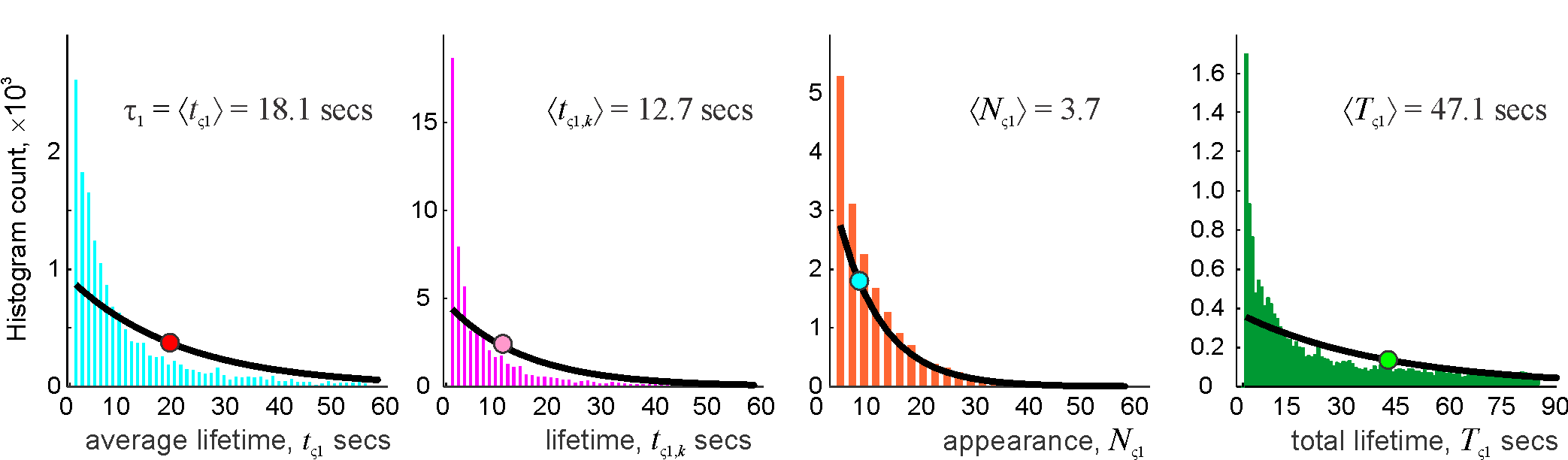
Figure S1: The statistics for the flickering connections in the cells assemblies. The statistics of the mean lifetimes $t_{\varsigma_{1}}$, individual lifetimes $t_{\varsigma_{1},k}$, number of appearances $N_{\varsigma_{1}}$ and the total existence periods $T_{\varsigma_{1}}$ of the $1D$ subsimplexes of the coactivity complex $\mathcal{F}_{\varpi}$, which is the links of the coactivity graphs $G(\varpi_{n})$, representing connections in the simulated cell assemblies. In all cases, the mean net existence period equals approximately to the product of the mean lifetime by the mean number of appearances $\langle T_{\varsigma_{1}}\rangle\approx\langle N_{\varsigma_{1}}\rangle\langle t_{\varsigma_{1},k}\rangle$.

The distribution of the maximal simplexes’ lifetimes $\delta t_{\varsigma,k}$ as a function of their dimensionality shows that higher-dimensional simplexes (and hence the higher-order cell assemblies) are shorter lived than the low order cell assemblies (Fig. 4C). The histogram of the mean lifetimes $t_{\varsigma}=\langle\delta t_{\varsigma,k}\rangle_{k}$ is closely approximated by the exponential distribution (Fig. 4D), which suggests that the duration of the cell assemblies’ existence can be characterized by a half-life $\tau$. The individual lifetimes $\delta t_{\varsigma,k}$, the number of appearances $N_{\varsigma}$, and net existence time $\Delta T_{\varsigma}=\sum_{k}\delta t_{\varsigma,k}$ of the maximal simplexes and of pairwise connections are also exponentially distributed (see Fig. 4E and Fig. S1). As expected, the mean net existence time approximately equals to the product of the mean lifetime and the mean number of the cell assembly’s appearance $\langle\Delta T_{\varsigma}\rangle\approx\langle N_{\varsigma}\rangle\langle\delta t_{\varsigma,k}\rangle$.

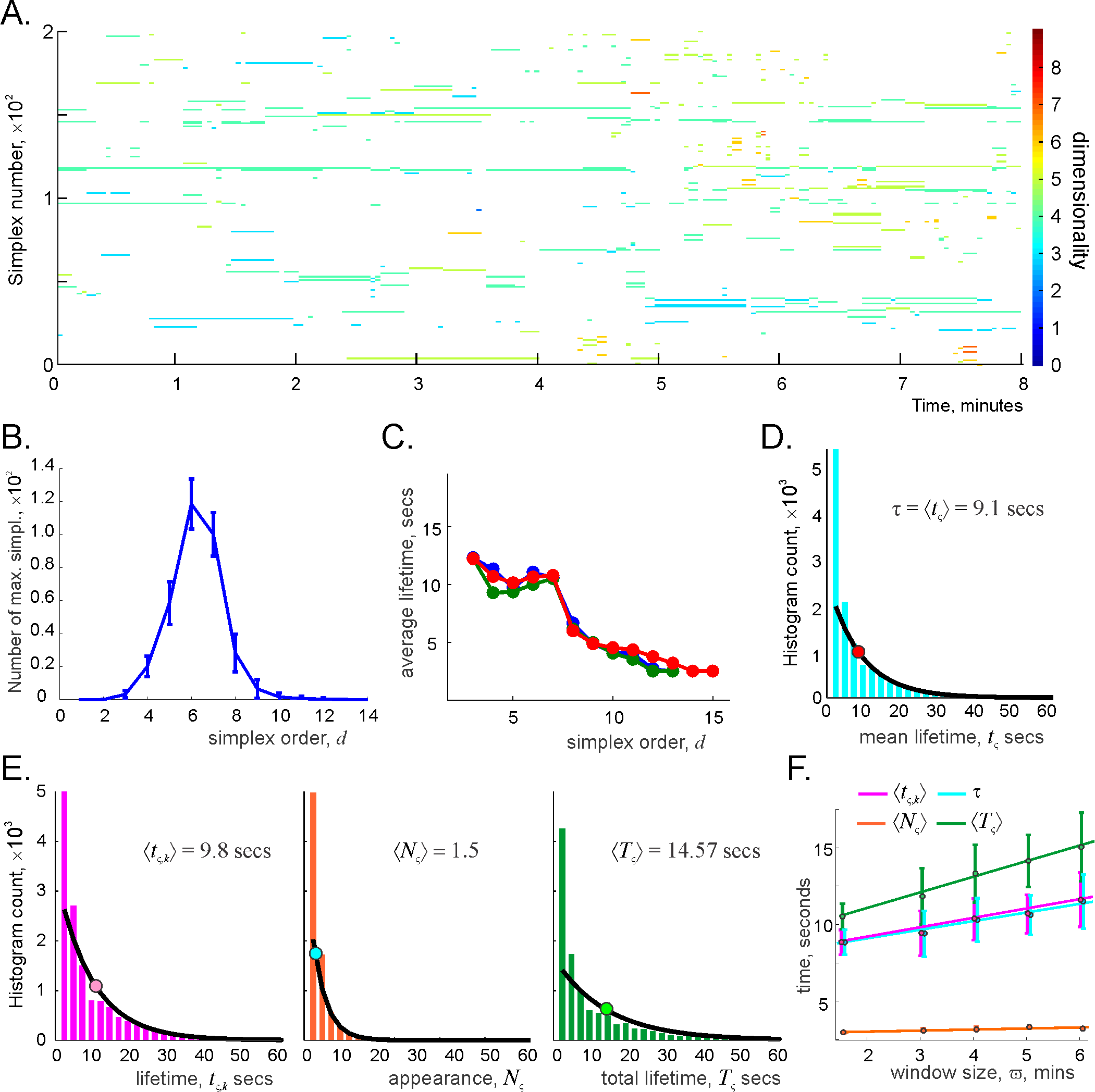
Figure 4: Fluctuating simplexes. (A) Maximal simplex timeline diagram: each strike represents a timeline of a particular maximal simplex $\varsigma$, computed for the coactivity window $\varpi=4$ min. There are about $N_{\varsigma}=320$ maximal simplexes at every given timestep (first 200 are enumerated along the $y$-axis), whereas the total number of maximal simplexes observed during the entire navigation period is about 11,000. The color of the timelines marks the order of $\varsigma$ (colorbar on the right). Notice that the simplexes of lower orders generally persist over longer intervals. (B) Number of maximal simplexes as a function of their order has a Gaussian shape with the mean $d=7$ and standard deviation $\Delta_{d}\approx\pm 2$, suggesting that a typical cell assembly contains about seven neurons and about two neurons may appear or disappear in it at a given moment. (C) Average existence time of the maximal simplexes tends to decay with increasing order. An exception is provided by the lowest order ($1D$) connections, which rarely appear as independently and quickly become absorbed into higher order maximal simplexes. (D) Histogram of the maximal simplexes’ individual average lifetimes $\tau_{\varsigma}$ fits with the exponential distribution with mean $\tau=9$s, defining the half-life of the simulated cell assemblies for this $\varpi$. (E) Histogram of the maximal simplexes’ lifetimes $t_{\varsigma,k}$, i.e., histogram of the lengths of all intervals between consecutive appearance and disappearance of the maximal simplexes, the histogram of the number of simplex-births $N_{\varsigma}$ and the histogram of the total existence periods $T_{\varsigma}$ fit with their respective exponential distributions. The mean number of simplex’ appearances $\langle N_{\varsigma}\rangle\approx 1.5$ shows that most maximal simplexes appear only once or twice, though some maximal simplexes may appear 20 times or more. Notice that the mean net existence period $\langle T_{\varsigma}\rangle\approx 14.57$s is approximately equal to the product of the mean lifetime and the mean number of appearances $\langle T_{\varsigma}\rangle\approx\langle N_{\varsigma}\rangle\langle t_{\varsigma,k}\rangle$. (F) As the size of the memory window $\varpi$ increases, the lifetimes, half-lives, and net existence periods of the maximal simplexes grow linearly with $\varpi$.

Fig. 4F shows how these parameters depend on the width of the integration window. As $\varpi$ widens, mean lifetime $t_{\varsigma}$ of maximal simplexes (and hence its half-life and the net lifetime) grows linearly, whereas the number of appearances $\langle N_{\varsigma}\rangle$ remains nearly unchanged. The latter result is natural since the frequency with which the cell assemblies ignite is defined by how frequently the animal visits their respective cell assembly fields, i.e., the domains where the corresponding sets of place fields overlap Babichev1 ). This frequency does not change significantly if the changes in $\varpi$ do not exceed the characteristic time required to turn around the maze and revisit cell assembly fields, in this case ca. $1-2$ min. Thus, the model produces a population of rapidly changing cell assemblies; in the simulated case $\tau\approx 9$ seconds, which is close to the experimental range of values Buzsaki1 . This allows us to address our main question: can a network of transient cell assemblies encode the topology of the environment?

Flickering coactivity complex. We next studied the flickering coactivity complex $\mathcal{F}_{\varpi}$ formed by the pool of fluctuating maximal simplexes. First, we observed that the size of $\mathcal{F}_{\varpi}$ does not fluctuate significantly across the rats’ navigation time. As shown in Fig. 5A, the number of maximal simplexes $N_{\varsigma}(\mathcal{F}_{\varpi}(t))$ fluctuates within about $4\%$ of its mean value. The fluctuations in the number of coactive pairs $N_{2}(\mathcal{F}_{\varpi}(t))$ is even smaller: $3\%$ of the mean, and the variations in number of the third order simplexes $N_{3}(\mathcal{F}_{\varpi}(t))$ are about $7\%$ of the mean. To quantify the structural changes in $\mathcal{F}_{\varpi}$, we computed the number of maximal simplexes that are present at time $t_{i}$ and missing at time $t_{j}$, yielding the matrix of asymmetric distances, $d_{ij}=N_{\varsigma}(\mathcal{F}_{\varpi}(t_{i})\ \mathcal{F}_{\varpi}(t_{j}))$ for all pairs $t_{i}$ and $t_{j}$ (see Methods and Fig. 5B). The result suggests that as temporal separation $|t_{i}-t_{j}|$ increases, the differences between $\mathcal{F}_{\varpi}(t_{i})$ and $\mathcal{F}_{\varpi}(t_{i})$ rapidly accumulate, meaning that the pool of maximal simplexes shared by $\mathcal{F}_{\varpi}(t_{i})$ and $\mathcal{F}_{\varpi}(t_{i})$ rapidly thins out. After about $50$ timesteps ($|i-j|>50$) the difference is about $95\%$ (Fig. 5B).

Since the coactivity complexes are induced from the pairwise coactivity graph $G$ as clique complexes, we also studied the differences between the coactivity graphs at different moments of time by computing the normalized distance between the coactivity matrices (see Methods). The results demonstrate that the differences in $G$, i.e., between $G(t_{j})$ and $G(t_{i})$, accumulate more slowly with temporal separation than in $\mathcal{F}_{\varpi}$: after about two minutes the connectivity matrices differ by about $10-15\%$ (Fig. 5C).

The Fig. 5D shows the asymmetric distance between two consecutive coactivity complexes $\mathcal{F}_{\varpi}(t_{i})$ and $\mathcal{F}_{\varpi}(t_{i+1})$, and the asymmetric distance between the starting and a later point $\mathcal{F}_{\varpi}(t_{1})$ and $\mathcal{F}_{\varpi}(t_{i})$, normalized by the size of $\mathcal{F}_{\varpi}(t_{1})$ as a function of time. The results suggest that, although the sizes the coactivity complexes at consecutive time steps do not change significantly, the pool of the maximal simplexes in $\mathcal{F}_{\varpi}$ is nearly fully renewed after about two minutes. In other words, although the coactivity complex changes its shape slowly, the integrated changes across long periods are significant (compare Fig. 5E with Fig. 2B). Biologically, this implies that the simulated cell assembly network, as described by the model, completely rewires in a matter of minutes.

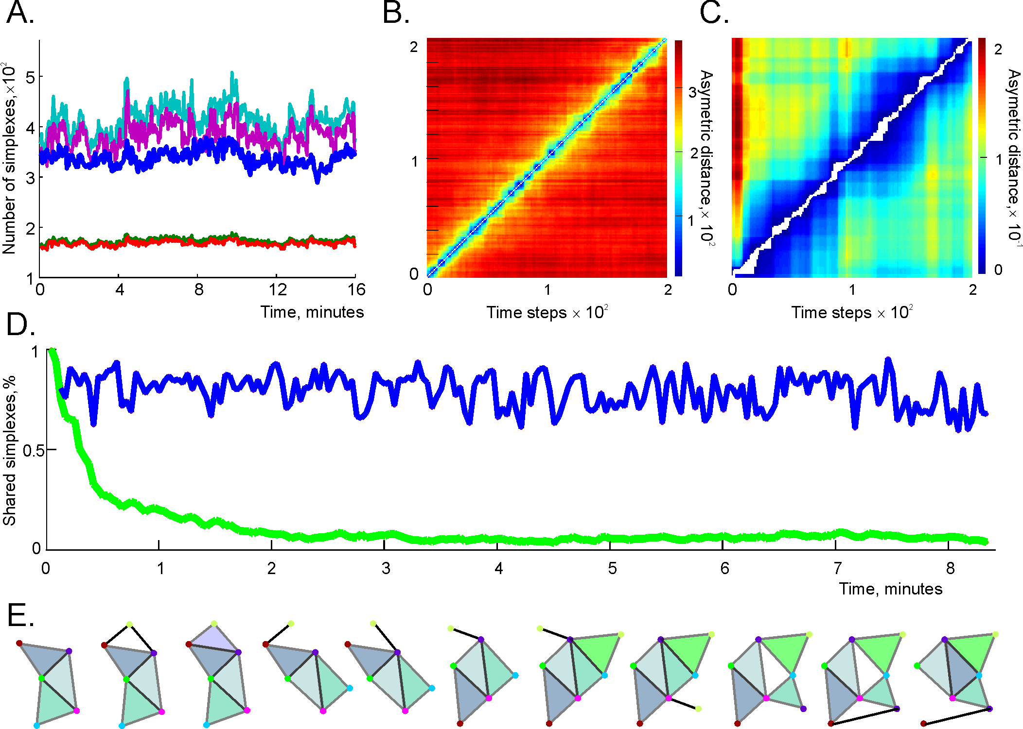
Figure 5: Behavior of the flickering coactivity complex computed for the memory window width $\varpi=4$ min, shifted over $\Delta t=2.5$ secs steps. (A) The number of maximal simplexes in $\mathcal{F}_{\varpi}$ (blue trace) fluctuates within $4\%$ of the mean value of $N_{\varsigma}=320$. The number of the $1D$ simplexes $N_{1}(\mathcal{F}_{\varpi})$ (red trace) and the number of the $1D$ simplexes appearing in consecutive windows (i.e., links shared by $\mathcal{F}_{\varpi}(t_{i})$ and $\mathcal{F}_{\varpi}(t_{i-1})$, green trace) fluctuate within a $3\%$ bound. The fluctuations in the number of $2D$ subsimplexes ($N_{2}(\mathcal{F}_{\varpi})$, light blue trace) and the number of $2D$ simplexes shared by two consecutive windows (purple trace) do not exceed $7\%$ of the mean. $N_{1}(\mathcal{F}_{\varpi})$ and $N_{2}(\mathcal{F}_{\varpi})$ are scaled down by a factor of 10 to fit the scale of the figure. (B) The asymmetric distance between $\mathcal{F}_{\varpi}(t_{i})$ and $\mathcal{F}_{\varpi}(t_{j})$ is defined as the number of the maximal simplexes at moment $t_{i}$ which are missing at the moment $t_{j}$ for all pairs ($t_{i}$, $t_{i}$). As the temporal separation $|t_{i}-t_{j}|$ grows, the asymmetric distance between $\mathcal{F}_{\varpi}(t_{i})$ and $\mathcal{F}_{\varpi}(t_{j})$ rapidly increases. (C) The matrix of similarity coefficients $r_{ij}$ between the weighted coactivity graphs at different moments of time. For close moments $t_{i}$ and $t_{j}$ the differences between $G(t_{i})$ and $G(t_{j})$ are small, but as time separation grows, the differences accumulate, though not as rapidly as with the coactivity complexes. (D) At each $t_{i}$ the blue line shows the proportion of maximal simplexes present at the previous time, $t_{i-1}$. The green line shows the proportion of maximal simplexes contained at the start (in $\mathcal{F}_{\varpi}(t_{1}))$ that remain in the coactivity complex at the later time $\mathcal{F}_{\varpi}(t_{i})$. The population of simplexes changes by about $0.95\%$ in about 2 min. (E) A schematic illustration of the changes of the coactivity complex’s shape: the fluctuations induce permanent restructurings. No skeletal structure, similar to that in the “expected” scenario shown in Fig. 2B, is preserved.

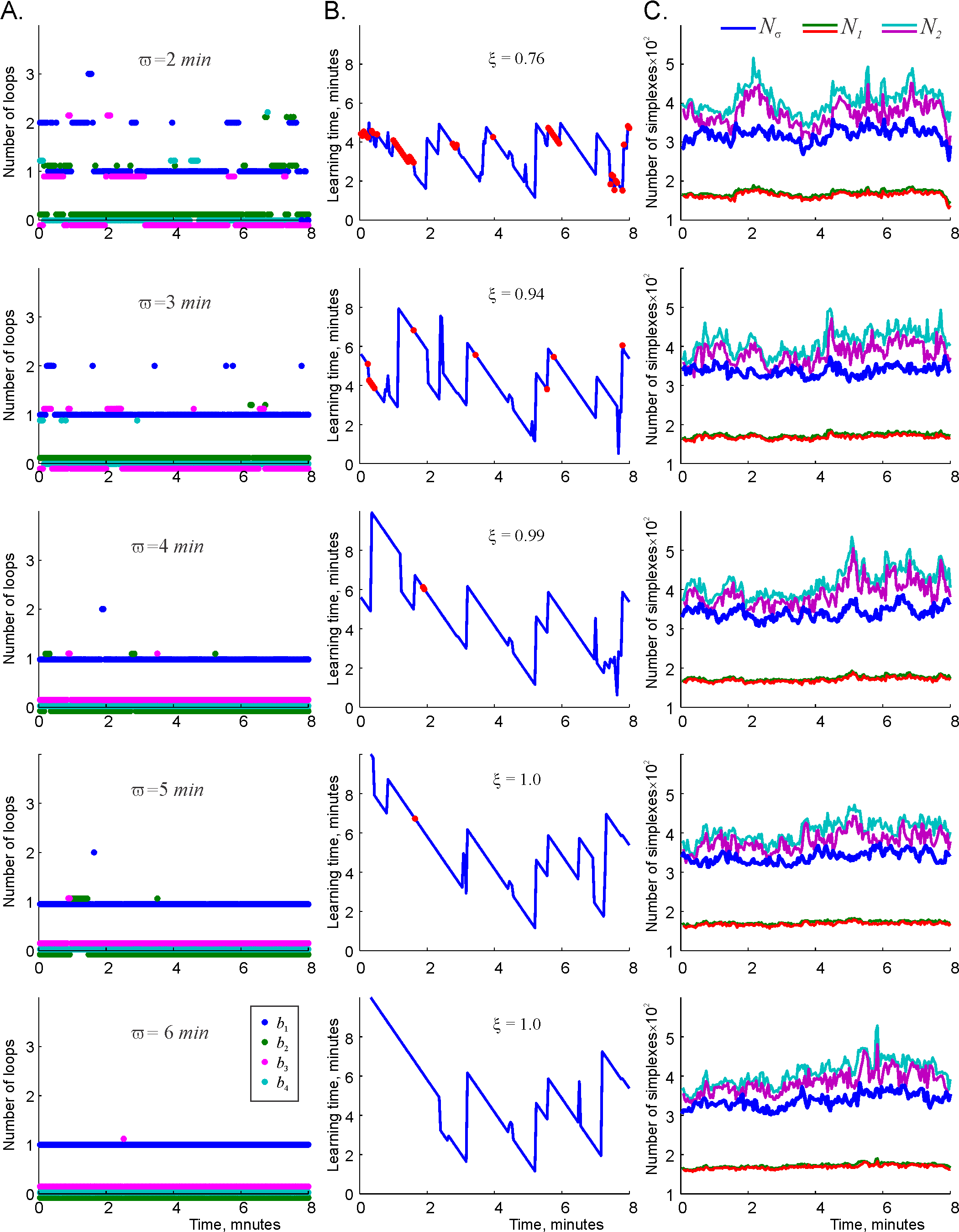
Figure S2: Flickering coactivity complex as a function of time. (A) As the coactivity integration window $\varpi$ increases, the topological fluctuations in the coactivity complex $\mathcal{F}_{\varpi}$ are suppressed. (B) The corresponding learning times $T_{\min}$. Red dots mark the moments when the map acquires a non-physical topological barcode. As the coactivity window $\varpi$ grows, the topological fluctuations are suppressed and the number of failures decreases. Notice that the learning time remains high immediately after the areas as the failures are suppressed. At $\varpi\approx 5$ min, when the mean half-life of a simulated cell assembly is about $\tau_{\varsigma}\approx 10$ secs (Fig. 4F), the map retains a topologically correct shape at all times. (C) Variations in the size of the coactivity complex $\mathcal{F}_{\varpi}$ reduce with increasing $\varpi$.

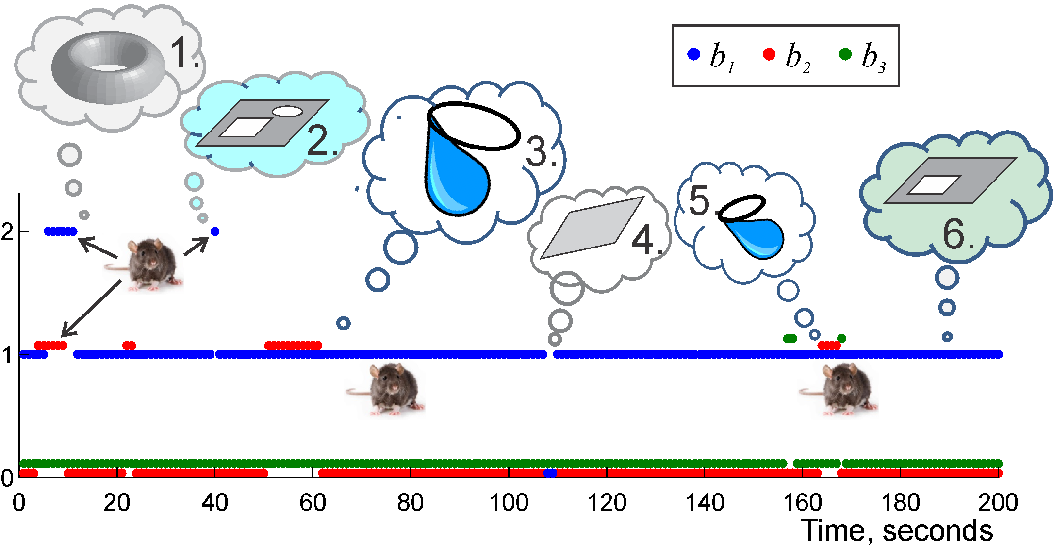
Figure S4: Topological fluctuations in the hippocampal map. As in the case illustrated in Fig. 6, we assume that the map forms one single piece at all times, hence its $0$-th Betti number $b_{0}=1$ is not shown. At the moment when the Betti numbers assume values $b_{1}=2$, $b_{2}=1$ and $b_{n>2}=0$, the hippocampal map warps into a shape that is topologically equivalent to a torus (Fig. 3C). At the moment when $b_{1}=2$ while $b_{n>1}=0$, the map contains an extra $1D$ loop indicating an extra gap in $\mathcal{F}_{\varpi}$. At the times when $b_{1}=b_{2}=1$ while $b_{n>2}=0$, the map contains a $2D$ bulge and a non-contractible cycle fused together (since $b_{0}=1$!). For most times, the topological type of $\mathcal{F}_{\varpi}$ coincides with the topological type of the simulated rat’s environment, $b_{1}=1$, $b_{n>1}=0$.

Topological analysis of the flickering coactivity complex exhibits a host of different behaviors. First, we start by noticing that the 0th and the higher-order Betti numbers always assume their physical values $b_{0}=0$, $b_{n>4}=0$, whereas the intermediate Betti numbers $b_{1}$, $b_{2}$, $b_{3}$ and (for small $\varpi$s) $b_{4}$ may fluctuate (Fig. 6A and Fig. S2). Thus, despite the fluctuations of its simplexes, the flickering complex $\mathcal{F}_{\varpi}$ does not disintegrate into pieces and remains contractible in higher dimensions ($D>3$). Biologically, this implies that the topological fluctuations in the simulated hippocampal map are limited to $1D$ loops, $2D$ surfaces and $3D$ bubbles. For example, an occurrence of $b_{1}=2$ value indicates the appearance of an extra (non-physical) $1D$ loop that surrounds a spurious gap in the cognitive map (Fig. 1A). On the other hand, at the moments when $b_{1}=0$, all $1D$ loops in $\mathcal{F}_{\varpi}$ are contractible, i.e., the central hole is not represented in the simulated hippocampal map. The moments when $b_{n>2}>0$ indicate times when the flickering complex $\mathcal{F}_{\varpi}$ contains non-physical, non-contractible multidimensional topological surfaces. One can speculate about the biological implications of these fluctuations, see Fig. S4.

As the coactivity window increases, the fluctuating topological loops become suppressed and vice versa. As the integration window shrinks, the fluctuations of the topological loops intensify (Fig. 6). This tendency could be expected, since the cell assembly lifetimes reduce as the integration window shrinks and increase as the coactivity integration window grows (Fig. 4F). However, a nontrivial result suggested by Fig. 6 is that the topological parameters of the flickering complex can stabilize completely, even though its maximal simplexes keep appearing and disappearing, or “flickering.” At $\varpi\approx 6$ minutes, the Betti numbers of $\mathcal{F}_{\varpi}$ remain unchanged (Fig. 6A), whereas the lifetime of its typical simplex is about 10 seconds (Fig. 4F). Biologically, this implies that a stable hippocampal map can be encoded by a network of transient cell assemblies, i.e., that the ongoing synaptic plasticity in the hippocampal network does not necessarily compromise the integrity of the large-scale representation of the environment.

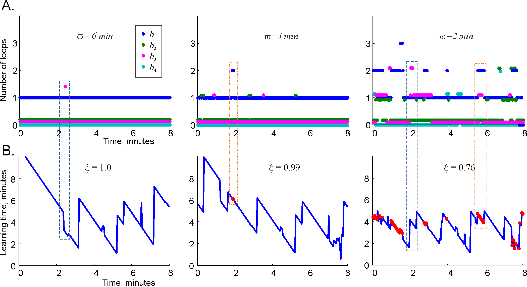
Figure 6: Stability of large-scale topological information. (A) The low-dimensional Betti numbers $b_{1}$, $b_{2}$, $b_{3}$ as a function of discrete time, computed for three coactivity integration windows, $\varpi=2$ min, $\varpi=4$ min, and $\varpi=6$ min. The $0$-th Betti number, $b_{0}=1$, remains stable at all times and is therefore not shown. At sufficiently large coactivity windows, $\varpi\sim 4-6$ minutes, the topological fluctuations become suppressed and the large-scale topological information remains stable, even though the characteristic lifetime of a maximal simplex in the coactivity complex $\mathcal{F}_{\varpi}$ is about $10$ secs (Fig. 4C). As the integration window narrows, the topological fluctuations intensify (Fig. S2). (B) The variation in the time required to extract the topological information increases as the coactivity integration window narrows. At $\varpi=2$ min, the complex $\mathcal{F}_{\varpi}$ fails to produce the correct topological information in $24\%$ of the cases (convergence score $\xi=0.76$). The failing moments are marked by red dots. As the memory window increases to $\varpi=4$ min, the topological mapping fails in only $1\%$ of the cases. As the memory window increases to $\varpi=6$ min, the failing points disappear. Here we compute the most conservative estimate for the learning time $T_{\min}$ to be the time required to establish the correct topology only in the dimensions that may contain physical obstructions, $0D$ and $1D$. Therefore, the points where $T_{\min}$ diverges are marked by appearances of spurious $1D$ loops (encapsulated into red dashed boxes across panels). The points where the learning time rapidly changes are often accompanied by the appearance or disappearance of higher dimensional topological loops (blue dashed boxes).

Local learning times. If the information about the detected place cell coactivities is retained indefinitely, the time required for producing the correct topological barcode of the environment $T_{\min}$ may be computed only once, starting from the onset of the navigation, and used as the low-bound estimate for the learning time PLoS ; Arai . In the case of a rewiring (transient) cell assembly network, the pool of encoded spatial connectivity relationships is constantly renewed. As a result, the time required to extract the large-scale topological signatures of the environment from place cell coactivity becomes time-dependent and its physiological interpretation also changes. $T_{\min}(t_{k})$ now defines the period over which the topological information emerges from the ongoing spiking activity at every stage of the navigation.

As shown in Fig. 6B, the proportion $\xi$ of “successful” coactivity integration windows, i.e., those windows in which $T_{\min}$ assumes a finite value, depends on their width $\varpi$. For small $\varpi$, the coactivity complex frequently fails to reproduce the topology of the environment (Fig. 6A). As $\varpi$ grows, the number of failing points, i.e., those for which $T_{\min}(t_{k})>\varpi$, reduces due to the suppression of topological fluctuations. The domains previously populated by the divergent points are substituted with the domains of relatively high but still finite $T_{\min}(t_{k})$. For sufficiently large coactivity windows ($\varpi>6$ minutes), such divergent points become exceptional: the correct topological information exists at all times, even though period required to produce this information is time-dependent.

The time dependence of $T_{\min}(t_{k})$ exhibits abrupt rises and declines, with characteristic $45^{\circ}$ slants in-between. The rapid rises of $T_{\min}(t_{k})$ correspond to appearances of obstructions in the coactivity complex $\mathcal{F}_{\varpi}$ (and possibly higher-dimensional surfaces) that temporarily prevent certain spurious loops from contracting. As more connectivity information is supplied by the ongoing spiking activity, the coactivity complex $\mathcal{F}_{\varpi}$ may acquire a combination of simplexes that eliminates these obstructions, allowing the unwanted loops to contract and yielding the correct topological barcode. Thus, Fig. 6B suggests that the dynamics of the coactivity complex is controlled by a sequence of coactivity events that produce or eliminate topological loops in $\mathcal{F}_{\varpi}$, while the $45^{\circ}$ slants in $T_{\min}(t_{k})$ represent “waiting periods” between these events (since with each window shift over $\Delta t$, the local learning time decreases by exactly the same amount).

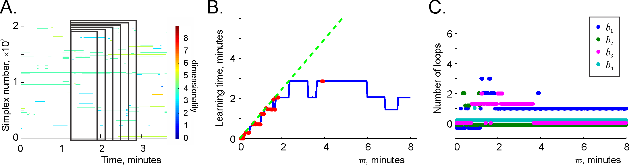
Figure 7: Stability the large-scale topological information. (A) A schematic illustration of the growing coactivity window $\varpi$, superimposed over a fragment of the maximal simplex timeline diagram. (B) The learning times $T_{\min}(\varpi_{k})$ computed within the growing coactivity window. The learning times computed within narrow coactivity windows either diverge ($T_{\min}(\varpi_{k})>\varpi$) or converge barely ($T_{\min}(\varpi_{k})\approx\varpi$). As $\varpi$ exceeds a certain critical value $\varpi_{c}$ (for the simulated place cell ensemble, $\varpi_{c}\approx 4-6$ minutes), the learning time $T_{\min}(\varpi_{k})$ stops increasing and begins to fluctuate around a certain mean value $T_{\min}=\langle T_{\min}(\varpi_{k})\rangle_{k}$. This value is independent of the coactivity window width and hence represents a parameter-free characterization of the mean time required to extract topological information from place cell coactivity. (C) The low-dimensional Betti numbers $b_{1}$, $b_{2}$, $b_{3}$ and $b_{4}$ as a function of the coactivity integration window width $\varpi$. As $\varpi$ exceeds a critical value $\varpi_{c}$, the Betti numbers $b_{n}$ stabilize, indicating suppression of the topological fluctuations in $\mathcal{F}_{\varpi}$.

It should be noticed that the network’s failure to produce a topological barcode at a particular moment, i.e., within a particular integration window $\varpi_{k}$, is typically followed by a period of successful learning. This implies that the rudimentary forgetting mechanism incorporated into the model, whereby the removal of older connectivity relationships from $\mathcal{F}_{\varpi}$ as newer relationships are acquired, allows correcting some of the accidental connections that that may have been responsible for producing persistent spurious loops at previous steps. In other words, a network capable of not only accumulating, but also forgetting information, exhibits better learning results.

Thus, the process of extracting the large-scale topology of the environment should be quantified in terms of the mean learning time $T_{\min}=\langle T_{\min}(t_{k})\rangle_{k}$ and its variance $\Delta T_{\min}/T_{\min}$, which does not exceed $40\%$ (typically $\Delta T_{\min}/T_{\min}\approx 20\%$). This suggests that $T_{\min}$ provides a statistically sound characteristics of the information flow across the simulated cell assembly network.

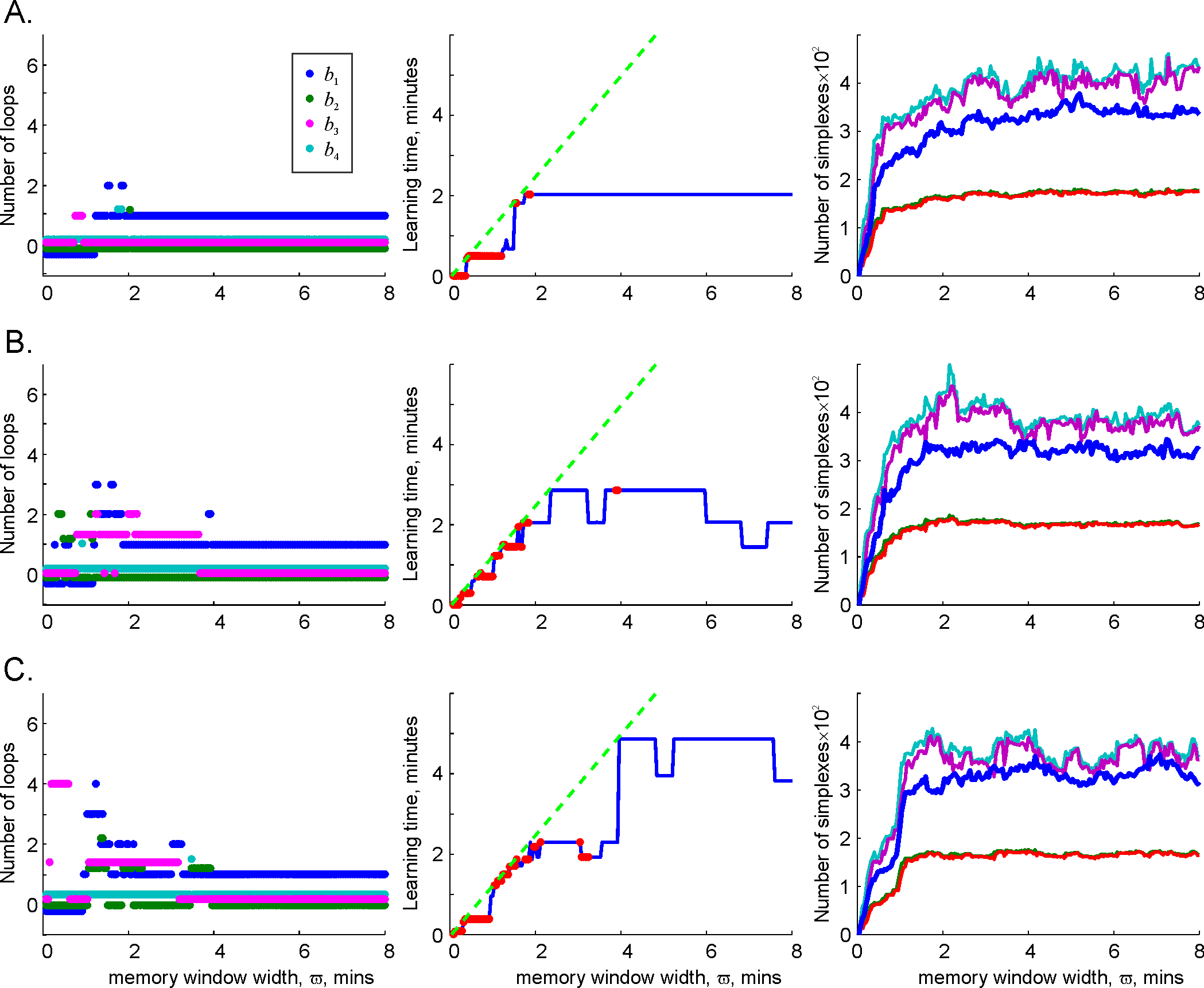
Figure S3: Growing memory window. (A) If the coactivity window is placed at a timepoint with few topological fluctuations, the Betti numbers $b_{1}$, $b_{2}$, $b_{3}$ and $b_{4}$, and the learning time quickly stabilize. The last panel indicates that size of the coactivity complex $\mathcal{F}_{\varpi}$ grows as a function of $\varpi$ and then acquires a stable size. (B) At a typical temporal domain, the behavior of the “asymptotic” coactivity complex $\mathcal{F}_{\varpi}$ exhibits stronger topological fluctuations and the learning time fluctuates as a function of increasing $\varpi$. (C) In the locations in which the topological fluctuations are strong, the Betti numbers of the flickering coactivity complex $\mathcal{F}_{\varpi}$ take longer to stabilize and the learning time may retain high values for longer periods, before returning to the typical regime shown on panel B.

To better understand how the learning time depends on the memory width, we tested the dependence of $T_{\min}$ on the size of the coactivity integration window $\varpi$. We fixed the position of several coactivity integration windows $\varpi_{k}$ and expanded their right side, $\varpi_{k}^{(1)}>\varpi_{k}^{(2)}>...>\varpi_{k}^{(q)}$ (Fig. 7 and Fig. S3). As one would expect, small values of $\varpi$ generated many failing points, whereas the learning times $T_{\min}(t_{k})$ computed for the successful trials remained nearly equal to $\varpi$, i.e., the width of the narrow integration windows was barely sufficient for producing the correct barcode $\mathfrak{b}(\mathcal{E})$. However, as $\varpi$ grows further, $T_{\min}$ stops increasing and, as $\varpi$ exceeds a certain critical value $\varpi_{c}$ (typically about five or six minutes), the learning time begins to fluctuate around a mean value $T_{\min}=\langle T_{\min}(t_{k})\rangle$ of about two minutes. In other words, for sufficiently large coactivity windows $\varpi>\varpi_{c}$, the learning times become independent of the model parameter $\varpi$ and therefore provides a parameter-free characterization of the time required by a network of place cell assemblies to represent the topology of the environment, whereas $\varpi_{c}$ defines the time necessary to collect the required spiking information (Fig. S4).

IV Discussion

Fundamentally, the mechanism of producing the hippocampal map depends on two key constituents: on the timing of the action potentials produced by the place cells and by the way in which the spiking information is processed by the downstream networks. A key determinant for the latter is the synaptic architecture of the cell assembly network, which changes constantly due to various forms of synaptic and structural plasticity: place cell assemblies may emerge in cell groups that exhibit frequent coactivity or disband due to lack thereof. The latter phenomenon is particularly significant: since the hippocampal network is believed to be one of the principal memory substrates, frequent recycling of synaptic connections may compromise the integrity of its net function. For example, the existence of many-to-one projections from the CA3 to the CA1 region of the hippocampus suggests that the CA1 cells may serve as the readout neurons for the assemblies formed by the CA3 place cells Carr ; Johnson . Electrophysiological studies suggest that the recurrent connections within CA3 and the CA3-CA1 connections rapidly renew during the learning process and subsequent navigation Sasaki ; Keller . On the other hand, it is also well known that lesioning these connections disrupts the animal’s performance in spatial Lee1 ; Kim ; Kesner1 and nonspatial Eichenbaum1 ; Farovik learning tasks, which suggests that an exceedingly rapid recycling of functional cell groups may impair the net outcome of the hippocampal network, which is the hippocampal spatial map Madronal ; Gilbert ; Lee2 ; Steffenach .

The proposed model allows investigating whether a plastic, dynamically rewiring network of place cell assemblies can sustain a stable topological representation of the environment. The results suggest that if the intervals between consecutive appearance and disappearance of the cell assemblies are short, the hippocampal map exhibits strong topological fluctuations. However, if the cell assemblies rewire sufficiently slowly, the information encoded in the hippocampal map remains stable despite the connectivity transience in its neuronal substrate. Thus, the plasticity of neuronal connections, which is ultimately responsible for the network’s ability to incorporate new information McHugh ; Leuner ; Dupret ; Schaefers , does not necessarily degrade the information that is already stored in the network. These results present a principal development of the model outlined in PLoS ; Arai ; Babichev1 from both a computational and a biological perspective.

Physiological vs. schematic learnings. The schematic approach proposed in Schemas allows describing the process of spatial learning from two perspectives: as training of the synaptic connections within the cell assembly network—referred to as physiological learning in Schemas —or as the process of establishing large-scale topological characteristics of the environment, referred to as “schematic,” or “cognitive,” learning. The difference between these two concepts is particularly apparent in the case of the rewiring cell assembly network, in which the synaptic configurations may remain unsettled due to the rapid transience of the connections. On the other hand, schematic learning is perfectly well defined since the large-scale topological characteristics of the environment can be achieved reliably.

In fact, the model outlines three spatial information processing dynamics at the short-term, intermediate-term, and long-term memory timescales Cowan . First, local spatial connectivity information is represented in transient cell assemblies within several seconds. This timescale corresponds to the scope of memory processes that involve temporary maintenance of information produced by the ongoing neural spiking activity, commonly associated with short-term memory Cowan ; Hebb . The short-term memory capacity is around seven ($7\pm 2$, Miller ) items, corresponding in the model to the order of the simulated cell assemblies (Fig. 4B). The information about the large-scale connectivity of the environment is acquired and updated—the (mean) learning time $T_{\min}$, Figs. 6 and 7—is on the order of minutes, corresponding to intermediate-term memory timescale Eichenbaum2 ; Kesner2 . The persistent topological information, represented by the stable Betti numbers, may represent long-term memory.

V Methods

The rat’s movements were modeled in a small planar environment, similar to the arenas used in electrophysiological experiments (bottom of Fig. 1A). The trajectory covers the environment uniformly, without artificial favoring of one segment of the environment over another.

Place cell spiking activity is modeled as a stationary temporal Poisson process with a spatially localized Gaussian rate characterized by the peak firing amplitude $f_{c}$ and the place field size $s_{c}$ Barbieri . In the simulated ensemble of $N_{c}=300$ place cells, the peak firing amplitudes are log-normally distributed with the mode $f_{c}=14$ Hz and the place field sizes are log-normally distributed with the mode $s_{c}=17$ cm. The place cell spiking probability is modulated by the $\theta$-component of the extracellular field oscillations (mean frequency of $\sim 8$ Hz Buzsaki2 ) recorded in wild-type Long Evans rats (see Methods in eLife ). For more computational details see Methods in PLoS ; Arai .

The activity vector of a place cell $c$ is constructed by binning its spike trains into an array of consecutive coactivity detection periods $w$. If the time interval $T$ splits into $N_{w}$ such periods, then the activity vector of a cell $c$ over this period is $m_{c}(T)=[m_{c;1},...,m_{c;N_{w}}]$, where $m_{c;k}$ specifies how many spikes were fired by $c$ into the $k$-th time bin Babichev1 . The activity vectors of $N_{c}$ cells, combined as rows of a $N_{c}\times N_{w}$ matrix, form the activity raster $R$. A binary raster $B$ is obtained from the activity raster $R$ by replacing the nonzero elements of $R$ with 1.

Place cell spiking coactivity is defined as the firing that occurred over two consecutive $\theta$-cycles, which is an optimal coactivity detection period $w$ both from the computational Arai and from the physiological Mizuseki perspective. A coactivity $\rho$ of a pair of cells $c_{1}$ and $c_{2}$ can be computed as the formal dot product of their respective activity vectors $\rho_{c_{1}c_{2}}=m_{c_{1}}(T)m_{c_{2}}(T)$.

Shifting coactivity window. The spiking activity confined within the $k$-th coactivity integration window of size $\varpi$ produces a local binary raster $B_{k}$ of size $N_{c}\times N_{\varpi/w}$, where $N_{\varpi/w}=\lfloor\varpi/w\rfloor$. The coactivity integration window was shifted by the discrete time steps $\Delta t=10w\approx 2.5$s. Thus, in $n_{s}=\varpi/\Delta t$ steps, the local rasters $B_{k}$ and $B_{k+ns}$ cease to overlap during the four-minute-long coactivity integration window $n_{s}=96$.

Coactivity distances. For each window $\varpi_{n}$, we compute the coactivities of every pair of cells

$$\rho^{n}_{ij}=\sum_{k}B^{n}_{i_{k}}B^{n}_{j_{k}},$$

where $B^{n}_{i_{k}}$ is the “local” binary raster of coactivities produced within that window. To compare different local rasters, we compute the similarity coefficients between them

$$r_{mn}=\sum_{i.j}|\rho^{n}_{ij}-\rho^{m}_{ij}|/\sum_{i.j}|\rho^{n}_{ij}|,$$

where indexes $i$,$j$ run over all the cells in the ensemble, illustrated in Fig. 4C.

The cell assemblies were constructed within each memory window using the Method II of Babichev1 , which is computationally more stable, produces less maximal simplexes and yields correct vertex statistics for the simulated hippocampal network.

Topological analyses were implemented using the JPlex package JPlex .

VI Acknowledgments

We thank R. Phenix for his critical reading of the manuscript. The work was supported by the NSF 1422438 grant and by the Houston Bioinformatics Endowment Fund.

VII References

VIII Supplementary Figures

References

- (1) Tolman EC (1948) Cognitive maps in rats and men. Psychol Rev, 55: 189-208.
- (2) O’Keefe J, Nadel L (1978) The hippocampus as a cognitive map, New York: Clarendon Press; Oxford University Press. xiv, 570 pp.
- (3) Nadel L, Hardt O (2004) The spatial brain. Neuropsychology, 18: 473-476.
- (4) McNaughton BL, Battaglia FP, Jensen O, Moser EI, Moser MB (2006) Path integration and the neural basis of the ’cognitive map’. Nat Rev Neurosci 7: 663-678.
- (5) Best PJ, White AM, Minai A (2001) Spatial processing in the brain: the activity of hippocampal place cells. Ann. Rev. Neurosci., 24, 459-486.
- (6) Brown EN, Frank LM, Tang D, Quirk MC, Wilson MA (1998) A statistical paradigm for neural spike train decoding applied to position prediction from ensemble firing patterns of rat hippocampal place cells. J Neurosci, 18, pp. 7411-7425.
- (7) Guger C, Gener T, Pennartz C, Brotons-Mas J, Edlinger G, et al. (2011) Real-time Position Reconstruction with Hippocampal Place Cells. Front Neurosci, 5.
- (8) Carr MF, Jadhav SP, Frank LM (2011) Hippocampal replay in the awake state: a potential substrate for memory consolidation and retrieval, Nat. Neurosci., 14, pp. 147-153.
- (9) Pfeiffer BE, Foster DJ (2013) Hippocampal place-cell sequences depict future paths to remembered goals, Nature, 497, pp. 74–79 (2013).
- (10) Dragoi G, Tonegawa S (2013) Distinct preplay of multiple novel spatial experiences in the rat. Proceedings of the National Academy of Sciences.
- (11) Dragoi G, Tonegawa S (2011) Preplay of future place cell sequences by hippocampal cellular assemblies. Nature, 469, 397-401.
- (12) Gothard KM, Skaggs WE, McNaughton BL (1996) Dynamics of mismatch correction in the hippocampal ensemble code for space: interaction between path integration and environmental cues, J Neurosci., 16, 8027-8040.
- (13) Leutgeb J, Leutgeb S, Treves A, Meyer R, Barnes C, McNaughton B, et al(2005) Progressive transformation of hippocampal neuronal representations in “morphed” environments, Neuron, 48, pp. 345-358.
- (14) Wills TJ, Lever C, Cacucci F, Burgess N, O’Keefe J (2005) Attractor dynamics in the hippocampal representation of the local environment, Science, 308, pp. 873-876.
- (15) Touretzky DS, Weisman WE, Fuhs MC, Skaggs WE, Fenton AA, et al. (2005) Deforming the hippocampal map. Hippocampus, 15: 41-55.
- (16) Diba K, Buzsaki G (2008) Hippocampal network dynamics constrain the time lag between pyramidal cells across modified environments. J Neurosci., 28: 13448-13456.
- (17) Dabaghian Y, Brandt VL, Frank LM (2014) Reconceiving the hippocampal map as a topological template, eLife 10.7554/eLife.03476, pp. 1-17.
- (18) Alvernhe A, Sargolini F, Poucet B (2012) Rats build and update topological representations through exploration, Anim. Cogn., 15, pp. 359-368.
- (19) Poucet B, Herrmann T (2001) Exploratory patterns of rats on a complex maze provide evidence for topological coding. Behav Processes, 53: 155-162.
- (20) Wu X, Foster DJ (2014) Hippocampal Replay Captures the Unique Topological Structure of a Novel Environment. J Neurosci., 34: 6459-6469.
- (21) Harris KD, Csicsvari J, Hirase H, Dragoi G, Buzsaki G (2003) Organization of cell assemblies in the hippocampus, Nature, 424, pp. 552-556.
- (22) Buzsaki G (2010) Neural syntax: cell assemblies, synapsembles, and readers, Neuron, 68, pp. 362-385.
- (23) Babichev A, Cheng S, Dabaghian YA (2016) Topological schemas of cognitive maps and spatial learning. Front. Comput. Neurosci. 10.
- (24) Caroni P, Donato F, Muller D (2012) Structural plasticity upon learning: regulation and functions, Nat Rev Neurosci., 13, pp. 478-490.
- (25) Chklovskii DB, Mel BW, Svoboda K (2004) Cortical rewiring and information storage, Nature, 431, pp. 782-788.
- (26) Wang Y, Markram H, Goodman PH, Berger TK, Ma J, et al. (2006) Heterogeneity in the pyramidal network of the medial prefrontal cortex. Nat Neurosci, 9: 534-542.
- (27) Kuhl BA, Shah AT, DuBrow S, Wagner AD (2010) Resistance to forgetting associated with hippocampus-mediated reactivation during new learning. Nat Neurosci., 13: 501-506.
- (28) Murre JMJ, Chessa AG, Meeter M (2013) A mathematical model of forgetting and amnesia. Frontiers in Psychology, 4.
- (29) Atallah BV, Scanziani M (2009) Instantaneous Modulation of Gamma Oscillation Frequency by Balancing Excitation with Inhibition. Neuron, 62: 566-577.
- (30) Bartos M, Vida I, Jonas P (2007) Synaptic mechanisms of synchronized gamma oscillations in inhibitory interneuron networks. Nat Rev Neurosci., 8: 45-56.
- (31) Mann EO, Suckling JM, Hajos N, Greenfield SA, Paulsen O (2005) Perisomatic Feedback Inhibition Underlies Cholinergically Induced Fast Network Oscillations in the Rat Hippocampus In Vitro. Neuron, 45: 105-117.
- (32) Whittington MA, Traub RD, Kopell N, Ermentrout B, Buhl EH (2000) Inhibition-based rhythms: experimental and mathematical observations on network dynamics. Int J Psychophysiol., 38: 315-336.
- (33) Bi G-q, Poo M-m (2001) Synaptic Modification by Correlated Activity: Hebb’s Postulate Revisited. Annu. Rev. Neurosci., 24: 139-166.
- (34) Magee JC, Johnston D (1997) A Synaptically Controlled, Associative Signal for Hebbian Plasticity in Hippocampal Neurons. Science, 275: 209-213.
- (35) Meck WH, Church RM, Olton DS (2013) Hippocampus, time, and memory. Behav. Neurosci.., 127: 655-668.
- (36) Clayton NS, Bussey TJ, Dickinson A (2003) Can animals recall the past and plan for the future? Nat. Rev. Neurosci., 4: 685-691.
- (37) Brown MF, Farley RF, Lorek EJ (2007) Remembrance of places you passed: Social spatial working memory in rats. Journal of Experimental Psychology: Animal Behavior Processes, 33: 213-224.
- (38) Dabaghian Y, Mémoli F, Frank L, Carlsson G (2012) A Topological Paradigm for Hippocampal Spatial Map Formation Using Persistent Homology, PLoS Comput. Biol., 8: e1002581.
- (39) Arai M, Brandt V, Dabaghian Y (2014) The Effects of Theta Precession on Spatial Learning and Simplicial Complex Dynamics in a Topological Model of the Hippocampal Spatial Map, PLoS Comput. Biol., 10: e1003651.
- (40) Curto C, Itskov V (2008) Cell groups reveal structure of stimulus space, PLoS Comput. Biol., 4: e1000205.
- (41) Aleksandrov PS (1965) Elementary concepts of topology. New York: F. Ungar Pub. Co. 63 pp.
- (42) Alexandroff P (1928) Untersuchungen Uber Gestalt und Lage Abgeschlossener Mengen Beliebiger Dimension. Annals of Mathematics., 30: 101-187.
- (43) Čech E (1932) Theorie generale del’homologie dans une space quelconque. Fundamenta mathematicae, 19: 149-183.
- (44) Dabaghian Y (2016) Maintaining Consistency of Spatial Information in the Hippocampal Network: A Combinatorial Geometry Model. Neural Comput: 1-21.
- (45) Novikov SP (2004) Discrete connections and linear difference equations. Tr. Mat. Inst. Steklova, 247: 186–201.
- (46) Babichev A, Memoli F, Ji D, Dabaghian Y (2015) Combinatorics of Place Cell Coactivity and Hippocampal Maps. Frontiers in Comput. Neurosci., 10:50
- (47) Mizuseki K, Sirota A, Pastalkova E, Buzsaki G (2009) Theta oscillations provide temporal windows for local circuit computation in the entorhinal-hippocampal loop, Neuron, 64, pp. 267-280.
- (48) Hoffmann K, Babichev A, Dabaghian Y (2016) Topological mapping of 3D space in bat hippocampi. In submission; posted on LANL arXiv:1601.04253.
- (49) K’́onig P, Engel AK, Singer W (1996) Integrator or coincidence detector? The role of the cortical neuron revisited. Trends Neurosci., 19: pp. 130-137.
- (50) Ratté S, Lankarany M, Rho Y-A, Patterson A, Prescott SA (2015) Subthreshold membrane currents confer distinct tuning properties that enable neurons to encode the integral or derivative of their input. Front. Cell Neurosci, 8.
- (51) Jonsson J (2008) Simplicial complexes of graphs. Berlin ; New York: Springer. xiv, 378 pp.
- (52) Babichev A, Dabaghian Y (2016) Persistent memories in transient networks. Springer Proceedings in Physics NDES Conference 2015.
- (53) Hatcher A (2002), Algebraic topology, Cambridge; New York: Cambridge University Press.
- (54) Ghrist R (2008) Barcodes: The persistent topology of data, Bulletin of the American Mathematical Society, 45, pp. 61-75.
- (55) Zomorodian AJ (2005), Topology for computing, Cambridge, UK ; New York: Cambridge University Press. xiii, 243 pp.
- (56) Edelsbrunner H, Harer J (2010) Computational topology : an introduction. Providence, R.I.: American Mathematical Society. xii, 241 pp.
- (57) Johnson A, Redish AD (2007) Neural Ensembles in CA3 Transiently Encode Paths Forward of the Animal at a Decision Point. J. Neurosci., 27: 12176-12189.
- (58) Sasaki T, Matsuki N, Ikegaya Y (2007) Metastability of Active CA3 Networks. The Journal of Neuroscience 27: 517-528.
- (59) Keller M, Both M, Draguhn A, Reichinnek S (2015) Activity-dependent plasticity of mouse hippocampal assemblies in vitro. Front. Neural Circuits, 9.
- (60) Lee I, Jerman TS, Kesner RP (2005) Disruption of delayed memory for a sequence of spatial locations following CA1- or CA3-lesions of the dorsal hippocampus. Neurobiol. Learn. Mem., 84: 138-147.
- (61) Kim SM, Frank LM (2009) Hippocampal lesions impair rapid learning of a continuous spatial alternation task. PLoS One, 4: e5494.
- (62) Kesner RP (2013) A process analysis of the CA3 subregion of the hippocampus. Front .Cell Neurosci., 7.
- (63) Eichenbaum H, Schoenbaum G, Young B, Bunsey M (1996) Functional organization of the hippocampal memory system. Proceedings of the National Academy of Sciences, 93: 13500-13507.
- (64) Farovik A, Dupont LM, Eichenbaum H (2010) Distinct roles for dorsal CA3 and CA1 in memory for sequential nonspatial events. Learn. Mem., 17: 12-17.
- (65) Madronal N, Delgado-Garcia JM, Fernandez-Guizan A, Chatterjee J, Kohn M, et al. (2016) Rapid erasure of hippocampal memory following inhibition of dentate gyrus granule cells. Nat. Commun., 7.
- (66) Gilbert PE, Kesner RP (2006) The role of the dorsal CA3 hippocampal subregion in spatial working memory and pattern separation. Behav. Brain Res., 169: 142-149.
- (67) Lee I, Hunsaker MR, Kesner RP (2005) The Role of Hippocampal Subregions in Detecting Spatial Novelty. Behav. Neurosci., 119: 145-153.
- (68) Steffenach H-A, Sloviter RS, Moser EI, Moser M-B (2002) Impaired retention of spatial memory after transection of longitudinally oriented axons of hippocampal CA3 pyramidal cells. Proceedings of the National Academy of Sciences, 99: 3194-3198.
- (69) McHugh TJ, Tonegawa S (2009) CA3 NMDA receptors are required for the rapid formation of a salient contextual representation. Hippocampus, 19: 1153-1158.
- (70) Leuner B, Gould E (2010) Structural Plasticity and Hippocampal Function. Annu. Rev. Psychol., 61: 111-140.
- (71) Dupret D, Fabre A, Döbrössy MD, Panatier A, Rodríguez JJ, et al. (2007) Spatial Learning Depends on Both the Addition and Removal of New Hippocampal Neurons. PLoS Biol., 5: e214.
- (72) Schaefers ATU, Grafen K, Teuchert-Noodt G, Winter Y (2010) Synaptic Remodeling in the Dentate Gyrus, CA3, CA1, Subiculum, and Entorhinal Cortex of Mice: Effects of Deprived Rearing and Voluntary Running. Neural Plast., 2010:11.
- (73) Cowan N (2008) What are the differences between long-term, short-term, and working memory? In: Wayne S. Sossin J-CLVFC, Sylvie B, editors. Prog. Brain Res.: Elsevier. pp. 323-338.
- (74) Hebb DO (1949) The organization of behavior; a neuropsychological theory. New York,: Wiley. xix, 335 p. p.
- (75) Miller GA (1956) The magical number seven, plus or minus two: some limits on our capacity for processing information. Psychol. Rev., 63: 81-97.
- (76) Eichenbaum H, Otto T, Cohen NJ (1994) Two functional components of the hippocampal memory system. Behavioral and Brain Sciences, 17: 449-472.
- (77) Kesner RP, Hunsaker MR (2010) The temporal attributes of episodic memory. Behav. Brain Res., 215: 299-309.
- (78) Barbieri R, Frank LM, Nguyen DP, Quirk MC, Solo V, Wilson M, et al(2004) Dynamic analyses of information encoding in neural ensembles, Neural Comput., 16, pp. 277-307.
- (79) Buzsaki G (2005) Theta rhythm of navigation: link between path integration and landmark navigation, episodic and semantic memory. Hippocampus, 15: 827-840.
- (80) JPlex freeware, http://comptop.stanford.edu/u/programs/jplex. ComTop group, Stanford University.