A study of the resonances $K_{0}^{*}(800)$ and $K_{0}^{*}(1430)$

Abstract

We study the scalar kaonic states $K_{0}^{\ast}(800)$ and $K_{0}^{\ast}(1430)$ by using a relativistic QFT Lagrangian in which only a single kaonic field corresponding to the well-established scalar state $K_{0}^{\ast}(1430)$ is considered and in which both derivative and non-derivative interaction terms are taken into account. Even if the scalar spectral function shows a unique peak close to $1.4$ GeV, we find two poles in the complex plane: $1.413\pm 0.002-i(0.127\pm 0.003)$ GeV, which is related to the seed quark-antiquark state $K_{0}^{\ast}(1430),$ and $0.746\pm 0.019-i(262\pm 0.014)$ GeV, which is an additional companion pole related to $K_{0}^{\ast}(800)$. As a further investigation for increasing $N_{c}$ confirms, $K_{0}^{\ast}(800)$ emerges as a dynamically generated four-quark object as a consequence of pion-kaon loops.

1 Introduction

The scalar resonance $K_{0}^{\ast}(1430)$ with $I(J^{P})=\frac{1}{2}(0^{+})$ is a well-established state listed in the summary table of the Particle Data Group (PDG) [1]. On the contrary, the scalar state $K_{0}^{\ast}(800)$, also with $I(J^{P})=\frac{1}{2}(0^{+})$ and known as $\kappa$ , still needs confirmation. The acceptance of the lightest $\kappa$ in the summary table of the PDG is important since it would allow to complete the nonet of the light scalar states below $1$ GeV.
The main aim of this work is to understand the nature of the two resonances $K_{0}^{\ast}(1430)$ and $K_{0}^{\ast}(800)$ using the quantum field theoretical model described in Ref. [2] (on which this proceedings is based). In particular, we shall concentrate on the existence and the properties of the latter state. The key ingredient of our theoretical approach is to consider at the same time both derivative and non-derivative interaction terms, see Sec. 2. We perform a fit of the four parameters of our model to the measured data points of $\pi K$ phase shift in the $I=1/2,J=0$ channel from Ref. [3] (See Sec. 3.1) and obtain a remarkably good agreement with the experiment. As a consequence of the fit, we determine the scalar kaonic spectral function up to $1.8$ GeV, in which only one single peak corresponding to $K_{0}^{\ast}(1430)$ appears. Namely, there is no peak corresponding to $K_{0}^{\ast}(800)$ but only a small enhancement in the corresponding energy region. Next, we calculate the coordinates of the poles on the complex plane. Despite the fact that we included only one “seed” state in the effective Lagrangian, we find two poles: one corresponding to the peak in the spectral function at $1.4$ GeV and thus to $K_{0}^{\ast}(1430)$, and one corresponding to the light $\kappa$. We get additional information about the nature of both resonances by studying the changes of the spectral function and the movement of the poles for increasing $N_{c}$: $K_{0}^{\ast}(1430)$ behaves as a $q\bar{q}$ state, while the light $\kappa$ is a dynamically generated state and as such a non-ordinary meson (see e.g. Refs. [4, 5, 6, 7, 8, 9] and refs. therein).

To confirm the correctness of our model, we study in Sec. 3.2 variations of it in which only the non-derivative or only the derivative interaction term is taken into account, respectively. We also studied variations of the form factor. In all cases we obtain a worse agreement with the experiment with respect to Sec. 3.1. It turns out that using both derivative and non-derivative terms is crucial to obtain a good description of experimental data. Finally, we summarize our results in Sec. 3.4.

2 The model

We use a relativistic interaction Lagrangian consisting of both derivative and nonderivative terms for a single $q\bar{q}$ scalar state denoted as $K_{0}^{\ast}$:

$$\mathcal{L}_{int}=aK_{0}^{\ast+}K^{-}\pi^{0}+bK_{0}^{\ast+}\partial_{\mu}K^{-}\partial^{\mu}\pi^{0}+\ldots\text{ ,}$$ (1)

where dots refer to complex conjugation and other members of the isospin multiplet. The model is naturally obtained as a piece of more complete chiral models, e.g. Ref. [10]. The decay width is given by:

$$\Gamma_{K_{0}^{\ast}}(m)=3\frac{\left|\vec{k}_{1}\right|}{8\pi m^{2}}\left[a-b\frac{m^{2}-M_{K}^{2}-M_{\pi}^{2}}{2}\right]^{2}F_{\Lambda}(m)\text{ ,}$$ (2)

where the pion and kaon masses are denoted as $M_{\pi}$ and $M_{K}$, and $\vec{k}_{1}$ is the three-momentum of the pion. The form-factor $F_{\Lambda}(m)=e^{-2\left|\vec{k}_{1}\right|^{2}/\Lambda^{2}}$, where $\Lambda$ stays for an energy scale, assures that calculations are finite. The propagator of $K_{0}^{\ast}$ reads

$$\Delta_{K_{0}^{\ast}}(p^{2}=m^{2})=\left[m^{2}-M_{0}^{2}+\Pi(m^{2})+i\varepsilon\right]^{-1}\text{ ,}$$ (3)

where $M_{0}$ is the bare mass of $K_{0}^{\ast}(1430)$ and $\Pi(m^{2})=\mathrm{Re}(m^{2})+i\mathrm{Im}(m^{2})$ is the one-loop contribution with one kaon and one pion circulating in it. We recall that the optical theorem implies that $\mathrm{Im}\Pi(m)=m\Gamma_{K_{0}^{\ast}}(m).$ The spectral function is given by:

$$d_{K_{0}^{\ast}}(m)=\frac{2m}{\pi}|\mathit{Im}\Delta_{K_{0}^{\ast}}(p^{2}=m^{2})|\text{ .}$$ (4)

The quantity $d_{K_{0}^{\ast}}(m)dm$ is the probability that the mass of the resonance is between $m$ and $m+dm.$ The normalization condition $\int_{0}^{\infty}d_{K_{0}^{\ast}}(m)\mathrm{dm}=1$ must hold. For the details of the mathematical treatment used here, we refer to [11]. In the next section we investigate the form of the spectral function, the poles of the propagator, and their dependence on the number of colors $N_{c}.$

3 Results

3.1 Fit to the phase shift data

We consider the $\pi K$ phase shift in the $I=1/2,J^{P}=0^{-}$ channel below $1.8$ GeV. Under the assumption that the $s$-channel contribution of the field $K_{0}^{\ast}$ dominates, the phase shift reads

$$\delta(m)=\frac{1}{2}\arccos\left[1-\pi\Gamma_{K_{0}^{\ast}}(m)d_{K_{0}^{\ast}}(m)\right]$$ (5)

Using the data of Ref. [3] (see also Ref. [12]) we perform a fit in order to determine four parameters of our model $a,b,$ $M_{0},$ and $\Lambda$, see Tab. 1. The result of the fit is presented in Fig. 1. We obtain a good agreement with the experimental data points ($\chi^{2}/d.o.f.=1.25$).

Table 1: The value of the parameters of our model.

Parameter	Value
$a$	$1.60\pm 0.22$ GeV
$b$	$-11.16\pm 0.82$ GeV-1
$m_{0}$	$1.204\pm 0.008$ GeV
$\Lambda$	$0.496\pm 0.008$ GeV

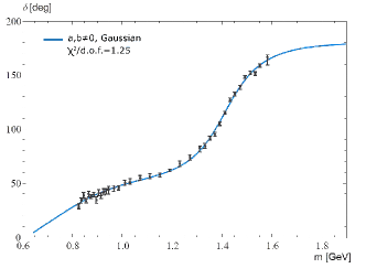
Figure 1: Result of the fit to the measured data points of the $\pi K$ phase shift in $I=1/2,J=0$ channel.

According to Eq. (4) and using the parameters reported in Tab. 1, we report in Fig. 2 the scalar kaonic spectral function up to $1.8$ GeV. We observe a single peak close to $1.4$ GeV corresponding to $K_{0}^{\ast}(1430),$ but there is no peak for $K_{0}^{\ast}(800)$ (only a small enhancement in the low energy is visible). For a comparison with the spectral function of the narrow Breit-Wigner type vector state $K^{\ast}(892)$ we refer to [13].

We study the large-$N_{c}$ limit of the spectral function according to the rescaling $a\longrightarrow\sqrt{3/N_{c}}a$, $b\longrightarrow\sqrt{3/N_{c}}b$, where $N_{c}$ is the number of colors, see Fig. 3. (Namely, the Lagrangian (1) contains a three-leg interaction term, whose amplitude scale as $1/\sqrt{N_{c}},$ e.g. Ref. [14]). The peak corresponding to $K_{0}^{\ast}(1430)$ becomes narrower and higher with decreasing $\lambda=3/N_{c}$, but the enhancement corresponding to $K_{0}^{\ast}(800)$ becomes smaller and finally disappears for increasing $N_{c}$.

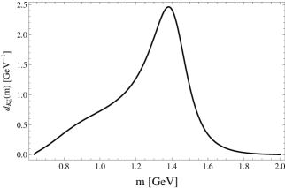
Figure 2: Scalar kaonic spectral function from Eq. (4).

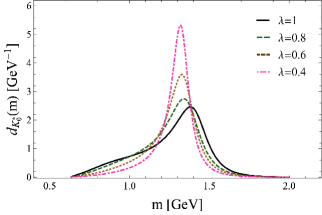
Figure 3: Scalar kaonic spectral function studied in large-$N_{c}$ limit.

As a next step we determine the positions of the poles in the complex plane. For the heavier state $K_{0}^{\ast}(1430)$ we get $1.413\pm 0.002-i(0.127\pm 0.003)$ GeV. In addition, we also find the lighter state $\kappa$: $0.746\pm 0.019-i(262\pm 0.014)$ GeV. In Fig. 5 we show the pole trajectories as function of $N_{c}$. The pole of $K_{0}^{\ast}(1430)$ moves toward to the real energy axis, while the pole of $K_{0}^{\ast}(800)$ moves away from it and disappears for $N_{c}\gtrsim 13$.

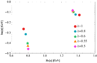
Figure 4: Positions of the poles of two resonances $K_{0}^{\ast}(1430)$ and $K_{0}^{\ast}(800)$ and their trajectories in large-$N_{c}$ limit.

In conclusion, even if in the effective Lagrangian of Eq. (1) a single $K_{0}^{\ast}$ seed state is considered, we obtain both scalar states $K_{0}^{\ast}(1430)$ and $\kappa\equiv K_{0}^{\ast}(800)$. Moreover, the behavior of the spectral function and the pole trajectories as function of $N_{c}$ show that $K_{0}^{\ast}(1430)$ is a predominantly quark-antiquark state, while the light $\kappa$ is generated dynamically, by the pion-kaon loop dressing a preformed quark-antiquark state. Accordingly, it disappears when the interaction strength is larger than a certain threshold.

3.2 Modifications of the model

We study different variations of our model in order to test the robustness of the results. First, we consider two different limits: one only with the derivative term ($a\neq 0$ and $b=0$ in Eq. (1)) and one only with the non-derivative term ($a=0$ and $b\neq 0$ in Eq. (1)). We perform the fits to the experimental data points of the phase shift, see Fig. 5. Both results of the fits, $\chi^{2}/d.o.f.=2.54$ and $\chi^{2}/d.o.f.=5.41$, are worsened w.r.t. the result in Sec. 3.1 (in which $\chi^{2}/d.o.f.=1.25$). Fig. 5 also shows that the derivative term is necessary to obtain a theoretical curve which is in qualitative agreement with the experiment.

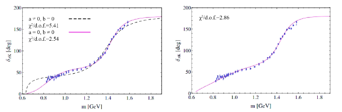
Figure 5: Fit results to the experimental points of the phase shift performed for different types of Lagrangian (left panel) and for modified form factor (right panel).

As a next step, we also test a different form of the form factor. Namely, although the Gaussian form used in Sec. 3.1 is typically used in such studies, there is no fundamental reason behind it. Therefore, we have repeated the fit with:

$$F_{\Lambda}(m)=e^{-2k^{4}(m)/\Lambda^{4}}\text{ .}$$ (6)

The result of the fit is presented in Fig. 5. It turns out that a qualitative agreement is obtained, but the $\chi^{2}$ is clearly worsened: $\chi^{2}=2.86.$ For the existence and positions of the poles for all these cases, we refer to [2].

4 Conclusions

In this work we have studied the properties of the scalar kaonic resonances $K_{0}^{\ast}(1430)$ and $K_{0}^{\ast}(800)$ according to the formalism described in Ref. [2]. The original Lagrangian contains a single scalar field, but because of hadronic quantum loops two poles emerge in the complex plane once that the parameters of the model are fitted to pion-kaon scattering data: one pole corresponds to the predominantly quark-antiquark resonance $K_{0}^{\ast}(1430),$ while the other one is an additional (non quark-antiquark) companion pole which corresponds to $K_{0}^{\ast}(800).$ While the former survives in the large–$N_{c}$ limit, the latter disappears. In the spectral function there is only a single peak, roughly corresponding to $K_{0}^{\ast}(1430);$ in the low-energy domain there is a small enhancement which is related to $K_{0}^{\ast}(800)$.

In the future, it will be interesting to apply these techniques to other enigmatic resonances, such as $D_{S0}^{*}(2317)^{\pm}$ and some of the newly discovered $X,$ $Y,$ and $Z$ states [15].


References

References

- [1] Olive K A et al. [Particle Data Group Collaboration] 2014 Chin. Phys. C 38 090001
- [2] Wolkanowski T, Soltysiak M and Giacosa F, arXiv:1512.01071 [hep-ph]
- [3] Aston D et al. 1988 Nucl. Phys. B 296 493.
- [4] van Beveren E, Rijken T A, Metzger K, Dullemond C, Rupp G and Ribeiro J E 1986 Z. Phys. C 30 615-620
- [5] Black D, Fariborz A H, Sannino F and Schechter J 1998 Phys. Rev. D 58 054012
-
[6]
Oller J A, Oset E and Pelaez J R, 1999
Phys. Rev. D 59 074001;
Pelaez J R 2004 Phys. Rev. Lett. 92 102001 -
[7]
Oller J A and Oset E, 1999
Phys. Rev. D 60 074023
[hep-ph/9809337]
Jamin M, Oller J A and Pich A, 2000 Nucl. Phys. B 587 331 [hep-ph/0006045] -
[8]
Pelaez J R 2004
Phys. Rev. Lett. 92 102001
Pelaez J R 2004 Mod. Phys. Lett. A 19 2879 [hep-ph/0411107] - [9] Fariborz A H, Pourjafarabadi E, Zarepour S and Zebarjad S M 2015 Phys. Rev. D 92 113002 [arXiv:1511.01623 [hep-ph]]
-
[10]
Parganlija D, Kovacs P, Wolf G, Giacosa F and
Rischke D H, 2012 Phys. Rev. D 87 014011;
Janowski S, Giacosa F and Rischke D H 2014 Phys. Rev. D 90 11 114005 [arXiv:1408.4921 [hep-ph]] - [11] Wolkanowski T, Giacosa F and Rischke D H 2016 Phys. Rev. D 93 no.1, 014002 [arXiv:1508.00372 [hep-ph]]
- [12] Ishida S, Ishida M, Ishida T, Takamatsu K and Tsuru T 1997 Prog. Theor. Phys. 98 621 [hep-ph/9705437]
- [13] Soltysiak M, Wolkanowski T and Giacosa F, arXiv:1604.01636 [hep-ph]
- [14] Witten E 1979 Nucl. Phys. B 160 57
- [15] Chen H X, Chen W, Liu X and Zhu S L, arXiv:1601.02092 [hep-ph]